An Iterative Hybrid Harmonics Detection Method Based on Discrete Wavelet Transform and Bartlett–Hann Window

Abstract

The current signal harmonic detection method(s) cannot reduce the errors in the analysis and extraction of mixed harmonics in the power grid. This paper designs a harmonic detection method based on discrete Fourier transform (DFT) and discrete wavelet transform (DWT) using Bartlett–Hann window function. It improves the detection accuracy of the existing methods in the low frequency steady-state part. In addition, it also separates the steady harmonics from the attenuation harmonics of the high frequency part. Simulation results show that the proposed harmonic detection method improves the detection accuracy of the steady-state part by 1.5175% compared to the existing method. The average value of low frequency steady-state amplitude detection of the proposed method is about 95.3375%. At the same time, the individual harmonic components of the signal are accurately detected and recovered in the high frequency part, and separation of the steady-state harmonics and the attenuated harmonics is achieved. This method is beneficial to improve the ability of harmonic analysis in the power grid.

1. Introduction

In recent years, as the smart grid enters the comprehensive construction stage, more and more power electronic equipment is put into operation. Among these power electronic devices, there are devices with nonlinear impedance characteristics, such as rectifiers, inverters, and phase speed control and voltage regulation devices. The use of non-linear power electronic equipment generates a lot of harmonic pollution, which causes significant voltage and current distortions and severely affects power quality. Therefore, accurate harmonic detection is of great significance for improving power quality and ensuring the reliability and safety of a power system [1,2].

The accuracy and response speed of harmonic detection depends on the method of harmonic detection. At present, the commonly used harmonic detection methods are as follows: analog filter method, instantaneous reactive power harmonic detection method, neural network harmonic detection method, wavelet transform harmonic detection method and Fourier transform harmonic detection method. The earliest harmonic measurements were achieved by analog filtering methods, which are very sensitive to the parameters of circuit components. Therefore, it is difficult to obtain ideal amplitude frequency and phase frequency characteristics, with large errors and poor real-time performance [3]. The harmonic detection method based on instantaneous reactive power usually uses a digital low pass filter, which has a large delay and directly affects the accuracy and speed of detection [4]. Based on the neural network harmonic detection method, the adaptive linear neural network method needs to accurately obtain the fundamental frequency to accurately extract the harmonic information in the signal [5]. The back-propagation neural network method requires a large number of sample data for training, and will have the disadvantages of training failure or slow convergence speed [6]. The harmonic detection method based on wavelet transform is suitable for the study of non-stationary signals. It has good time-frequency characteristics and is sensitive to transient signals. The analysis of different frequencies through multi-resolution improves the analysis accuracy and preserves the time domain information of the signal. However, the analysis accuracy of the harmonics in the steady state is not as good as that of the FFT, and the frequency is aliased, which will reduce the accuracy of the detection results [7,8]. The use of FFT algorithm to perform DFT solves the problem of a larger amount of calculation. However, DFT has spectrum leakage and fence effects, which will cause large errors in the analysis frequency and amplitude. The large errors and defects in the detection of non-steady-state signals limit the application of DFT in harmonic detection of power systems [9,10]. The research on the harmonic detection method based on Fourier transform is mainly focused on finding a window function with concentrated energy and rapid side lobe attenuation and an interpolation algorithm with higher performance. By analyzing the current mainstream harmonic detection methods, the most widely used discrete Fourier transform based harmonic detection methods and discrete wavelet transform based harmonic detection methods are selected. By analyzing the advantages of the DFT and DWT, some scholars have proposed a hybrid harmonic detection strategy combining two methods [11,12]. First, the original signal is decomposed into a high frequency part and low frequency part by wavelet transform (the Mallat algorithm), and the separation and extraction of low frequency steady-state harmonics and high frequency non-steady-state harmonics are realized. Because most of the steady-state harmonics exist in the low frequency part, few of the steady-state harmonics exist in the high frequency part. The non-steady-state harmonics in the high frequency part are composed of steady-state harmonics and attenuated harmonics. After each decomposition of original signal, the low frequency part can be repeatedly decomposed again. Each layer of decomposition decomposes the input signal of this layer into a low frequency approximate component part and a high frequency detailed part. In addition, the out sampling frequency of each stage can be halved. The significance of halving the sampling frequency is that it will not cause information loss.

This paper designs an improved harmonic detection method based on DFT and DWT using the Bartlett–Hann window function. According to reference [13], the Bartlett–Hann window is a linear combination of the Bartlett and Hanning windows. Taking into account its main lobe width and side lobe attenuation, it is more effective for detecting steady-state harmonics. For the high frequency part, based on the Hanning window DFT and DWT hybrid harmonic detection method, only the attenuation harmonic component is analyzed, and no consideration is given to whether the high frequency part containing the steady-state signal component and the attenuation harmonic component coexist. The method designed in this article can be divided into three cases for processing by analyzing the high frequency part. The steady-state harmonics in the high frequency part are distinguished from the transient harmonics, and the error of the steady-state harmonic component extraction is less than 5%. The amplitude of the attenuated harmonic component at the beginning is basically consistent with the theoretical amplitude. It can improve the detection accuracy of the hybrid detection strategy in the low frequency part, and separate and extract the doped steady-state harmonics from the non-steady-state harmonics in the high frequency part. Simulation experiments show that the algorithm designed in this paper has good harmonic detection accuracy for harmonic detection, and can achieve separation and extraction of high frequency parts.

The rest of this article is organized as follows. Section 2 introduces the principle of the hybrid harmonic detection method based on the Bartlett window DFT and DWT. Section 3 introduces the design of an improved method based on the Bartlett–Hann window DFT and DWT hybrid harmonic detection. Section 4 provides simulation results of test signals and test data. Section 5 summarizes this study.

2. Principles of Improved Harmonic Detection Methods

The Mallat algorithm uses the characteristics of multi-frequency analysis to decompose the signal and divides the signal into low frequency and high frequency parts. Add Bartlett–Hann window function interpolation DFT algorithm to realize the steady-state signal restoration and the existence of steady-state signals at high frequency. The DWT algorithm implements the reconstruction of non-steady signals. The principles of the DFT algorithm and the DWT algorithm are relatively common. The following mainly introduces the principles of the Mallat algorithm and the Bartlett–Hann window algorithm.

2.1. Mallat Algorithm

Wavelet transform can perform time-frequency analysis on signals because it has the ability of multi-resolution analysis [14,15]. According to the idea of multi-frequency analysis, the wavelet transform expansion formula:

$$\begin{array}{l}f(t)={\displaystyle \sum _{k=-\infty }^{\infty }{c}_{j,k}}\phi (t-k)+{\displaystyle \sum _{k=-\infty }^{\infty }{\displaystyle \sum _{j=0}^{\infty }{d}_{j,k}\psi (2^{j}t-k)}}\\ c_{j,k}=<s(n),{\phi }_{j,k}(n)>,d_{j,k}=<s(n),{\psi }_{j,k}(n)>\end{array}$$

(1)

where, $\phi (t)$ is a scale function, $\psi (t)$ is a wavelet function, orthogonal to each other, and together constitute the basis function of the wavelet transform. $c_{j,k}$ and $d_{j,k}$ are the decomposed components, $j$ is the scale factor, and $k$ is the displacement factor.

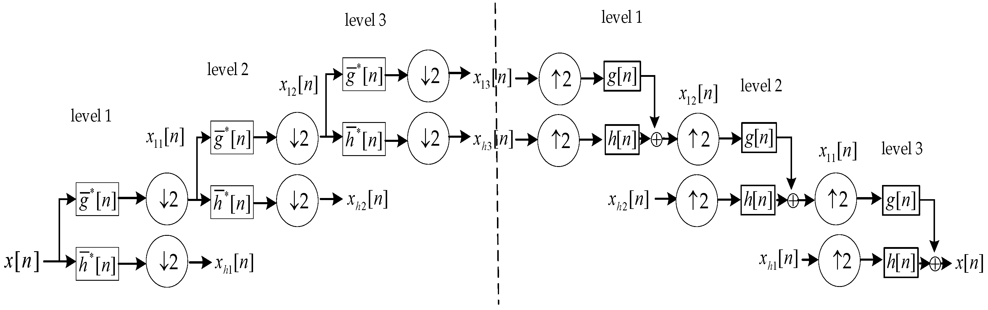
The Mallat algorithm is a fast wavelet transform algorithm based on analysis of resolution. It is also a mainstream method of using wavelet functions for decomposition and reconstruction. This method can be used to decompose and reconstruct time-varying parameters. The Mallat algorithm explains the physical meaning of scale function and wavelet function. During the decomposition process, the scale function is equivalent to a low pass filter (${\overline{g}}^{*}[n]$), retaining the main information of the signal. The wavelet function is equivalent to a high pass filter (${\overline{h}}^{*}[n]$), which retains the changes in the detail. In the reconstruction process, the low pass filter ($g[n]$) and the high pass filter ($h[n]$) are the reverse order of the decomposition process. The Mallat algorithm implements the decomposition and reconstruction of the three-layer discrete wavelet transform, as shown in Figure 1, where ${\overline{g}}^{*}[n]$ and ${\overline{h}}^{*}[n]$ are analysis filters, $g[n]$ and $h[n]$ are synthesis filters.

2.2. Bartlett–Hann Algorithm Principle

At present, research on harmonic detection methods based on discrete Fourier transform is mainly focused on finding window functions for fast decay of side lobes, and interpolation algorithms with higher performance. The Bartlett window is very similar to a triangular window as returned by the triang function—both are convolutions of two rectangles. However, the Bartlett window always has zeros at the first and last samples, while the triangular window is nonzero at those points. For odd values of n, the center n−2 points of bartlett (n) are equivalent to triang (n−2) [16]. The formula for the triangular window is shown in Equation (2), and the formula for the Bartlett window is shown in Equation (3).

$$\begin{array}{ll}n is an odd number:& \hspace{1em}n is an even number:\\ w(k)=\left\{\begin{array}{ll}\frac{2k}{n+1}& 1\le k\le \frac{n+1}{2}\\ \frac{2(n-k+1)}{n+1}& \frac{n+1}{2}\le k\le n\end{array}\right\}& \hspace{1em}w(k)=\left\{\begin{array}{ll}\frac{2k-1}{n}& 1\le k\le \frac{n}{2}\\ \frac{2(n-k+1)}{n}& \frac{n}{2}\le k\le n\end{array}\right\}\end{array}$$

(2)

$$\begin{array}{ll}n is an odd number:& n is an even number:\\ w(k)=\left\{\begin{array}{ll}\frac{2(k-1)}{n-1}& 1\le k\le \frac{n+1}{2}\\ 2-\frac{2(k-1)}{n-1}& \frac{n+1}{2}\le k\le n\end{array}\right\}& w(k)=\left\{\begin{array}{ll}\frac{2(k-1)}{n-1}& 1\le k\le \frac{n+1}{2}\\ \frac{2(n-k)}{n-1}& \frac{n}{2}\le k\le n\end{array}\right\}\end{array}$$

(3)

The Bartlett–Hann window is like the Bartlett, Hanning, and Hamming windows. This window has a main lobe at the origin and side edges that are gradually decaying on both sides. In fact, it is a linear combination of weighted Bartlett and Hanning windows [13,17]. Its near side lobes are lower than the Bartlett and Hanning windows, and its far side lobes are lower than the Bartlett and Hamming windows. Bartlett–Hann windows do not increase the width of the main lobe of the window compared to Bartlett or Hanning windows. According to reference [17], the time-domain expression used to calculate the Bartlett–Hann window is shown in Equation (4):

$$x(n)=0.62-0.48\left|(\frac{n}{N}-0.5)\right|+0.38\cos (2\mathsf{\pi }(\frac{n}{N}-0.5))$$

(4)

where $0\le n\le N$, the length of the window is $L=N+1$. Its frequency domain expression is as shown in Equation (5):

$$X({\mathrm{e}}^{\mathrm{j}\omega })=\{0.24X_{\mathrm{b}}(\omega )+0.38X_{\mathrm{R}}(\omega )+0.19X_{\mathrm{R}}(\omega -\frac{2\mathsf{\pi }}{N})+0.19X_{\mathrm{R}}(\omega +\frac{2\mathsf{\pi }}{N})\}{\mathrm{e}}^{-\mathrm{j}(\frac{N-1}{2})\omega }$$

(5)

where $X_{\mathrm{b}}(\omega )$ is the spectrum of the Bartlett window, and its expression is as shown in Equation (6):

$$X_b(\omega )=\frac{2}{N}{\left[\frac{\sin (\frac{N\omega }{4})}{\sin (\frac{\omega }{2})}\right]}^2$$

(6)

$X_{\mathrm{R}}(\omega )$ is the spectrum of a rectangular window, and its expression is as shown in Equation (7):

$$X_R(\omega )=\frac{\sin (\frac{N\omega }{2})}{\sin (\frac{\omega }{2})}$$

(7)

Compared with other windows, considering its main lobe width and side lobe attenuation speed, it is suitable for the window interpolation DFT algorithm, has better characteristics of suppressing spectral leakage, can reduce interference between harmonics, and improves the accuracy of signal analysis degree.

2.3. Comparison of Bartlett–Hann Windows and Common Windows

In order to verify the advantages of the Bartlett–Hann window, and compared with several common windows, common window functions include rectangular windows, triangular windows, Hanning windows, Heming windows, and Blackman windows. Different window functions have different effects on the frequency spectrum. The main reason is that different window functions produce different frequency spectrum leaks and different frequency resolution capabilities. The use of the DFT algorithm to calculate the frequency spectrum has a fence effect [18].

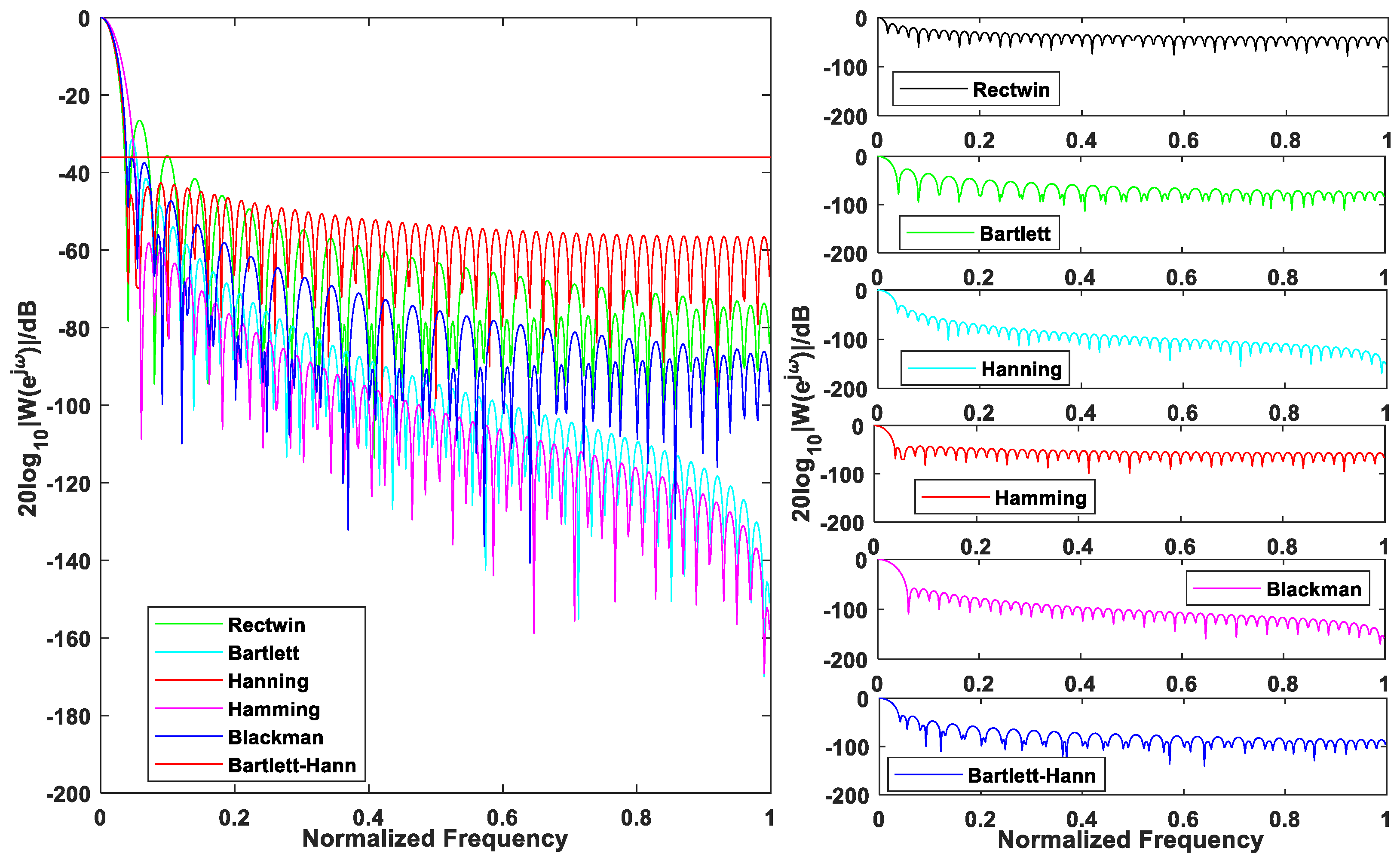
Both of the above defects cannot be eliminated. In this paper, we can choose different window functions to suppress their effects. The spectral leakage is related to the side lobes on both sides of the window function spectrum. If the height of the side lobes on both sides approaches 0 and the energy is relatively concentrated in the main lobe, closer to the true spectrum can be obtained. For the selection of the window function, the maximum effect of maintaining the maximum information and eliminating the side lobe should be to make the width of the main lobe in the window function spectrum as narrow as possible and the side lobe attenuation as large as possible [19]. The spectral comparison of Bartlett–Hann window and several common windows is shown in Figure 2.

It can be seen from the figure that the main lobe of the rectangular window is the most concentrated, but has the largest side lobe peak, and the side lobe attenuation speed is slow, the frequency recognition accuracy is high, and the amplitude recognition accuracy is low. The width of the main lobe of a triangular window is large, about twice that of a rectangular window, and the side lobes are small. The side lobe decays faster than a rectangular window. The width of the main lobe of a Hamming window is similar to that of a triangular window, but the side lobes are smaller and the side fading speed is fast. Both the Hamming window and the Hanning window are cosine windows. The Hamming window is an improved raised cosine window. The width of the main lobe is similar to that of the Hamming window. The decay speed is not as fast as the Hamming window. The main lobe width of the Blackman window is the largest of these common window functions, the side lobe is the smallest, and the side lobe decay rate is the fastest. Based on the comprehensive effect of windowing, the ratio of the Bartlett–Hann window to the rectangular window, Bartlett window, and Hanning window has the maximum side lobe minimum, and the maximum side lobe is −36 dB; compared with Bartlett and Hamming, the Bartlett–Hann window decays faster at farther side; Blackman has the widest main lobe. Although the side lobe decays fastest, its calculation is too large. In general, Bartlett–Hann windows have excellent performance in many aspects and are suitable for window interpolation DFT algorithms.

2.4. Comparison of Bartlett–Hann Windows and Common Windows

According to the actual situation of the power grid, the ideal fundamental frequency is 50 Hz, and the maximum amplitude of the fundamental wave is 1. According to the literature [20], a list of some harmonic parameters of the grid except the fundamental wave is shown in

Table 1. Some harmonic parameters except the fundamental wave in the power grid.

Number of Harmonic	2	3	4	5	6	7	8	9	10
Content(%)	0.5	5	0.4	3	0.6	2	0.2	3	0.5

.

According to Table 1, select the length of the sampling window in twelve signal cycles, set the number of sampling points to 1024, the sampling frequency to 2000 Hz, and the standard grid frequency of 50 Hz as the standard. A comparison has been made between the ordinary DFT algorithm and the interpolation DFT algorithm of Bartlett–Hann window function. The method of calculating relative error is used to reflect the deviation of the measured data from the actual value of the two methods, reflecting the credibility of the method. The calculation formula of absolute error and relative error is as follows:

$$\{\begin{array}{l}\Delta =\alpha -\beta \\ \delta =\Delta /\beta *100\%\end{array}$$

(8)

where, $\delta$ is a relative error, $\Delta$ is an absolute error, $\alpha$ is the measured value and $\beta$ is a theoretical value. The data are shown in

Table 2. Comparison of ordinary DFT algorithm and Bartlett–Hann window interpolation DFT algorithm.

Number of Harmonic	Relative Frequency Error (%)		Relative Amplitude Error (%)
	Common DFT	Bartlett–Hann Window Interpolation DFT	Common DFT	Bartlett–Hann Window Interpolation DFT
Fundamental	−2.34	−1.86	−14.52	−3.43
2	0.12	0.098	254.05	−1.02
3	0.9	−0.73	−27	−2.36
4	0.098	0.1	63.75	2.64
5	−0.39	−0.3906	−36.64	3.37
6	0.097	0.097	10.83	−0.83
7	0.035	0.034	−28.5	−4.28
8	0.098	0.098	38.25	−2.44
9	−0.0482	−0.0484	−21.67	−3.67
10	0.097	0.0976	8.4	−3

.

As can be seen from Table 2, the accuracy of the ordinary DFT algorithm is weaker than the Bartlett–Hann window function interpolation DFT algorithm. The relative error of the frequency detection of the ordinary DFT algorithm is less than 2.34%, while the relative error of the amplitude detection can reach 254.05%, which does not meet the national power quality standards. However, the interpolation DFT algorithm based on Bartlett–Hann window function has a relative error of less than 1.86% in frequency detection, and a relative error of less than 4.3% in amplitude detection. Therefore, the Bartlett–Hann window interpolation DFT algorithm is relatively accurate for detecting harmonics.

3. Design of Improved Harmonic Detection Method

3.1. Hybrid Harmonic Detection Method Based on Bartlett–Hann Window DFT and DWT

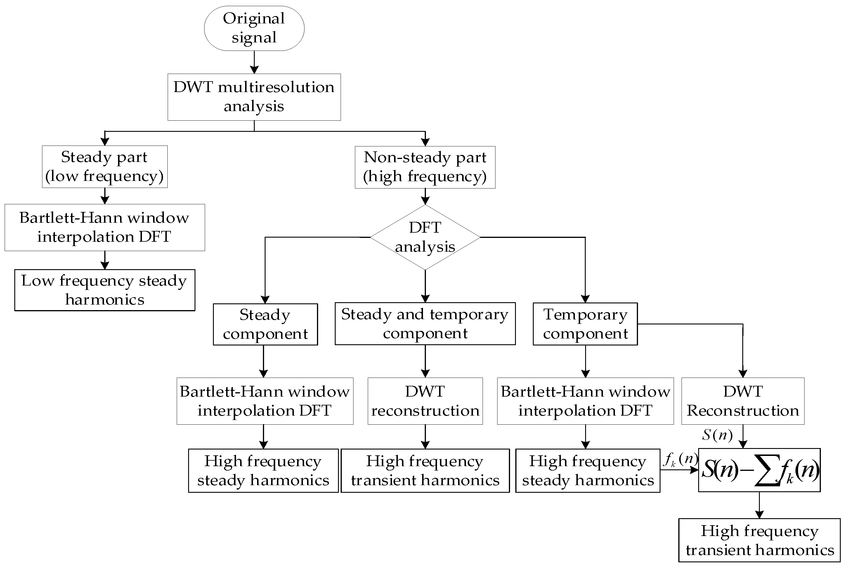
This paper designs an improved method based on DFT and DWT using Bartlett–Hann window function hybrid detection. The detection accuracy is improved, and the high frequency part harmonics are separated and extracted. The harmonic signal is decomposed into high frequency part and low frequency part by wavelet multi-resolution analysis. The steady-state part exists in the low frequency part, and the non-steady-state part exists in the high frequency part. According to the frequency band situation, the high frequency part may be doped with steady-state harmonic components, resulting in deviations in detection accuracy. For the low frequency steady-state part, we use a Bartlett–Hann window with better side lobe properties to implement windowed interpolation DFT processing to obtain low frequency steady-state components.

For the low frequency part, windowed interpolation is used to obtain the spectral information of the steady-state harmonic components. According to reference [17], assuming a harmonic signal $f(t)$ containing the $I$ th harmonic, and a uniform sampling frequency $F_s$, and according to the sampling theorem $f_s\ge 2F_{\max }$, a discrete-time signal is obtained as in Equation (9):

$$f(n)={\displaystyle \sum _{i=1}^I{V}_i\sin (\frac{2\pi f_i\cdot n}{f_s}+{\phi }_i)}$$

(9)

where $V_i$ is the amplitude of the $i$ th harmonic; $f_i$ is the frequency of the $i$ th harmonic; ${\phi }_i$ is the initial phase angle of the $i$ th harmonic.

Add a Bartlett–Hann window to the discrete-time signal $f(n)$ to obtain the windowed function $f_x(n)=f(n)x(n)$, where $x(n)$ is the window function, and do discrete-time Fourier Transform(DTFT) to obtain Equation (10):

$$F_x(i)={\displaystyle \sum _{n=-\infty }^{\infty }f(n)x(n)e^{-2\mathsf{\pi }fn}={\displaystyle \sum _{i=1}^I\left[\frac{V_i}{2\mathrm{j}}[e^{\mathrm{j}\phi i}\cdot X(\frac{2\mathsf{\pi }(f-f_i)}{f_s})-e^{-\mathrm{j}\phi i}\cdot X(\frac{2\mathsf{\pi }(f+f_i)}{f_s})]\right]}}$$

(10)

When estimating the $i$ th harmonic, if the influence of other component leakage on the $i$ th harmonic is ignored, discretize the formula to obtain Equation (11):

$$F_x(k\Delta f)=\frac{V}{2\mathrm{j}}{e}^{\mathrm{j}\phi }X(\frac{2\mathsf{\pi }(k\Delta f-f_i)}{f_s})$$

(11)

where in the discrete frequency interval $\Delta f=f_s/N$, $N$ is the data truncation length, and $X()$ is the Bartlett–Hann window spectrum. For the signal frequency $f_i$, $f_s$ is not a multiple of $f_i$, and is an asynchronous sampling.

For the high frequency part, considering whether it is doped with a steady-state signal, a Fourier transform is performed on the reconstructed high frequency part first, and three cases that may exist after the transformation are processed differently. Assume that the high frequency part after wavelet reconstruction is $S(n)$, the average value of all peaks in the first half of $S(n)$ is $S_1$, the average value of all peaks in the second half is $S_2$, and $(S_2-S_1)/S_2$ is the attenuation rate. The degree is considered as a function of decay. The discrete Fourier transform of $S(n)$ is $F(n)$. After extracting the parameters of $F(n)$, each harmonic is reduced to $f_k(n)$. The three possible situations are handled as follows:

(1)

Analysis of the reconstructed waveform from the wavelet transform shows that there is no attenuating signal in the high frequency part, but only the steady-state signal. In view of this situation, the parameters extracted from the data obtained by windowed interpolation DFT are used to restore the high frequency harmonics. The $f_k(n)$ obtained is the result of harmonic analysis.

(2)

The high frequency part contains only time-varying signals with a tendency to decay. In view of this situation, the reconstruction result $S(n)$ of the wavelet transform is used as the result of the final harmonic analysis.

(3)

There are both time-varying harmonic signals and steady-state harmonic signals in the high frequency part. In view of this situation, the parameters extracted from the data obtained by the windowed interpolation DFT are used to restore the high frequency harmonics to obtain $f_k(n)$, and sequentially perform difference processing with the high frequency signal $S(n)$ reconstructed by the wavelet. After each $S(n)-{\displaystyle \sum f_k(n)}$, the attenuation rate is recalculated. When the attenuation rate shows a decreasing trend or reaches a minimum or even a negative value, this indicates that $f_k(n)$ is an attenuation harmonic signal and is recorded as $f_k^{*}(n)$. According to $f_k^{*}(n)=S(n)-{\displaystyle \sum f_k(n)}$, it can restore time-varying harmonic signals.

The flowchart of the improved harmonic detection method is shown in Figure 3.

4. Simulation Test Analysis

4.1. Modeling and Analysis of Power Signals

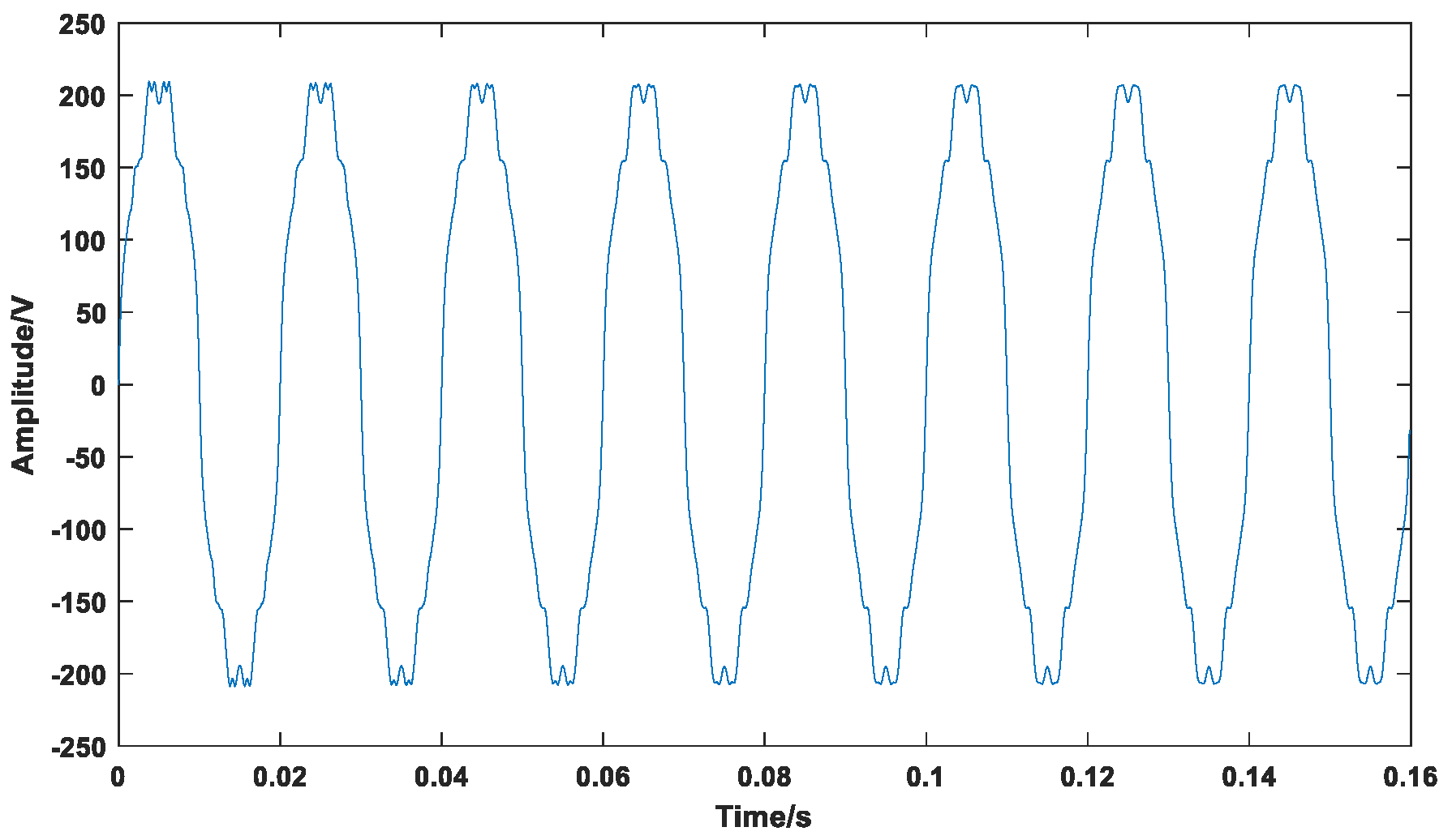
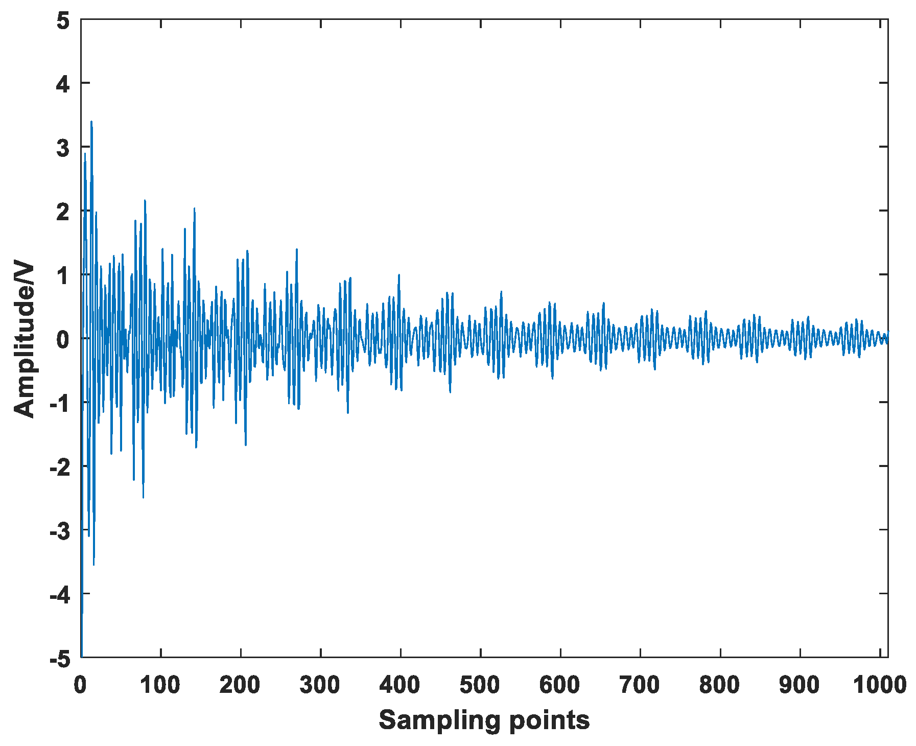
According to the power signal data, the common steady-state harmonics are the 3, 5, 7, 11, and 13 harmonics, which are also accompanied by some sudden changes, noise, and transient interference. Therefore, the signal model in this paper contains a 50 Hz fundamental wave component of 3, 5, 7, 11, 13, 19 harmonics, 23 and 33 harmonic attenuation components, and random noise $\sigma (t)$. Due to the main research on the separation and extraction of each harmonic in the signal, the relative delay in the transmission process of the power grid is not considered temporarily. The signal model can include the three cases mentioned in Section 3 in the case of decomposing three layers, so that conclusion is better proved. The complex harmonic signal model is shown in Equation (12).

$$\begin{array}{ll}S(t)& =220\sin (100\mathsf{\pi }t)+21\sin (300\mathsf{\pi }t)\\ & +15\sin (500\mathsf{\pi }t)+13\sin (700\pi t)\\ & +8\sin (1100\mathsf{\pi }t)+5\sin (1300\pi t)\\ & +3\sin (1900\mathsf{\pi }t)+3\sin (2300\mathsf{\pi }t)e^{-20t}\\ & +2\sin (3300\mathsf{\pi }t)e^{-20t}+0.2\sigma (t)\end{array}$$

(12)

In addition to the common steady-state harmonics, the signal $S(t)$ also contains an exponentially decaying harmonic at the beginning, and a random noise $\sigma (t)$ with random interference. The signal $S(t)$ waveform is shown in Figure 4.

According to the national standard power quality public network harmonics requirements for harmonic detection, the actual sampling frequency is 6400 Hz, and the number of sampling points is 1024 [12]. According to the characteristics of the harmonic model, the number of decomposition layers does not need to be too large, so the number of decomposition layers selected by this method is three layers, and multi-resolution analysis is performed on the signal $S(t)$. Taking into account the orthogonality and symmetry of the wavelet base, in order to make the band division effect better, the analysis wavelet used is db10. The decomposition and reconstruction calculation formula using the Mallat algorithm is as follows:

The wavelet transform decomposition formula is shown in Equation (13):

$$\begin{array}{l}{c}_n^k=\frac{1}{\sqrt{2}}{\displaystyle \sum _{j\in Z}{c}_j^{k-1}}{h}_{j-2n}^{*} \\ d_n^k=\frac{1}{\sqrt{2}}{c}_j^{k-1}{g}_{j-2n}^{*}\end{array}$$

(13)

The reconstruction formula is shown in Equation (14):

$$c_n^0={\displaystyle \sum _{k=1}^N({\displaystyle \sum _{j\in Z}{d}_j^k{g}_{j-2n}})+{\displaystyle \sum _{j\in Z}{c}_j^N{h}_{j-2n}}}$$

(14)

where, scale $k=1,2,\dots \dots N$, the maximum value of $k$ decomposition in this paper is 3. $h_j,g_j$ is a discrete filter, and the value of $j$ is limited in actual calculation. The transformation is from $c_n^0$ to $c_n^1$ and $d_n^1$. This is the first layer decomposition. The original signal is decomposed into A1 layer and D1 layer. The second layer decomposition is obtained from $c_n^1$ into $c_n^2$ and $d_n^2$, and the A1 layer is divided into A2 and D2 layers. In the same way, $c_n^N$ and $d_n^N$ can be obtained in the end. Reconstruction is the opposite of decomposition. First, $c_n^{N-1}$ is obtained from $c_n^N$ and $d_n^N$. Similarly, $c_n^0$ is finally synthesized. $c_n^N$ is the low frequency part and $d_n^N$ is the high frequency part.

In order to verify the algorithm proposed in this paper, the layers of the signal model are analyzed. The A3 layer is the low frequency steady-state component part, the D3 layer is the high frequency steady-state part, the D2 layer is the high frequency steady-state and attenuation component coexisting part, and the D1 layer is the high frequency attenuation component. The frequency of layer A1 is 1~1600 Hz, the frequency of layer D1 is 1600~3200 Hz; the frequency of layer A2 is 1~800 Hz, and the frequency of layer D2 is 800~1600 Hz; the frequency of layer A3 is 1~400 Hz, and the frequency of layer D3 is 400~800 Hz. The wavelet decomposition coefficients are shown in Figure 5.

4.2. Simulation Results of Low Frequency Part of Power Data

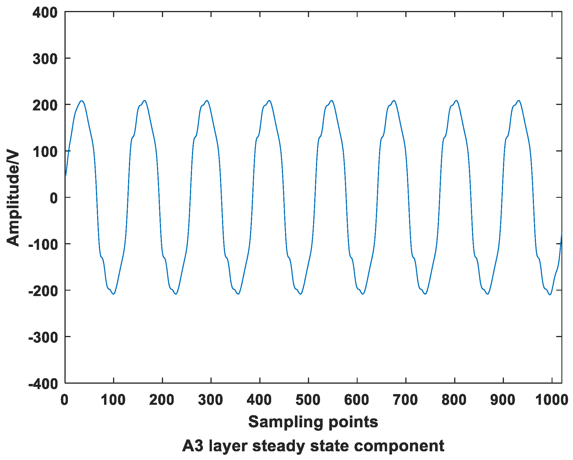
Decomposed by the Mallat algorithm, the frequency of the A3 layer is 1~400 Hz, including the fundamental wave and the 3, 5 and 7 low frequency steady-state harmonics. Therefore, the A3 layer is used as the low frequency part, and the A3 layer is reconstructed. The low frequency steady-state part of the A3 layer is shown in Figure 6.

The original method is based on the Hanning window function interpolation DFT and DWT mixed harmonic detection method, and the improved method is based on the DFT and DWT using the Bartlett–Hann window function mixed harmonic detection method. In order to compare the accuracy of low frequency part detection between the two, the low frequency steady state portion of the A2 layer after reconstruction is analyzed by the Hanning window function interpolation DFT algorithm and Bartlett–Hann window function interpolation DFT algorithm, respectively. The corresponding frequency spectrum is shown in Figure 7.

According to the proposed Bartlett–Hann window interpolation optimization and the literature [21], Hanning window interpolation optimization is compared with the theoretical value. Combining the spectrum analysis result in Figure 7, the DFT analysis frequency and amplitude of the low frequency steady state harmonic component fundamental wave, 3rd, 5th and 7th harmonics are obtained. The comparison is shown in

Table 3. Table of analysis results of steady-state harmonic components at low frequencies.

Number of Harmonic	Fundamental	3	5	7
Theory Frequency (Hz)	50	150	250	350
Actual Frequency (Hz)	50.78	148.44	250	351.56
Theory Amplitude (V)	220	21	15	13
Hanning Window Function Interpolation DFT Algorithm Amplitude (V)	218.68	20.87	14.59	10.43
Bartlett–Hann Window Function Interpolation DFT Algorithm Amplitude (V)	219.24	20.94	14.63	10.98

and the data obtained in the table are the average of three sets of data.

Table 3 presents the comparison between the proposed low frequency part using the Bartlett–Hann window interpolation DFT and the original method Hanning window interpolation with theoretical values. The steady-state harmonic component results obtained by the two detection methods are very close to the theoretical values. In order to make the test results more intuitive, amplitude accuracy and relative error are used to illustrate the accuracy of the two methods, as shown in

Table 4. Comparison table of analysis results of two methods.

Number of Harmonic		Fundamental	3	5	7	Average Value
Amplitude Accuracy(%)	Hanning Window Function Interpolation DFT Algorithm	99.4	98.38	97.27	80.23	93.82
	Bartlett–Hann Window Function Interpolation DFT Algorithm	99.65	99.71	97.53	84.46	95.3375
Relative Amplitude Error (%)	Hanning Window Function Interpolation DFT Algorithm	−0.6	−0.619	−2.73	−19.77	−5.93
	Bartlett–Hann Window Function Interpolation DFT Algorithm	−0.345	−0.286	−2.46	−15.53	−4.655

.

As can be seen from Table 4, the amplitude accuracy of the interpolation DFT algorithm of the Bartlett–Hann window function is about 95.3375%, and the relative error of the amplitude is less than 5%. The amplitude accuracy of the interpolation DFT algorithm of the Hanning window function is about 93.82%, and the relative error of the amplitude is less than 6%. It can be seen from the accuracy and relative errors that the Bartlett–Hann window function’s interpolation DFT algorithm has higher accuracy in detecting harmonics in the low frequency part, which is improved by about 1.5175%. Compared with the data in Table 2, the data in Table 2 directly analyzed the original signal, and the data in Table 4 analyze the data after hierarchical reconstruction, so the relative errors and accuracy are different.

4.3. Simulation Results of High Frequency Part of Power Data

There are steady-state harmonics and attenuation harmonics in the high frequency portion of the signal. The interpolation DFT and DWT mixed harmonic detection methods based on the Hanning window function can also restore the attenuated harmonic components through layering. If the signal in this frequency band are superimposed, this method cannot subdivide the frequency band. Therefore, the specific parameters of each harmonic cannot be distinguished, and the specific waveform of each harmonic cannot be reconstructed. The method proposed in this paper is based on the original method. It analyzes the harmonics in each frequency band to determine whether there are steady-state harmonics. Using the parameters extracted from the data obtained after windowed interpolation DFT, the harmonics at high frequencies perform the restore. According to the method in Section 3.1, the steady state component and the attenuation component of the high frequency part are separated and extracted. The following three sections will perform harmonic analysis on the three layers in turn.

4.3.1. High Frequency Steady-State Component Simulation Results

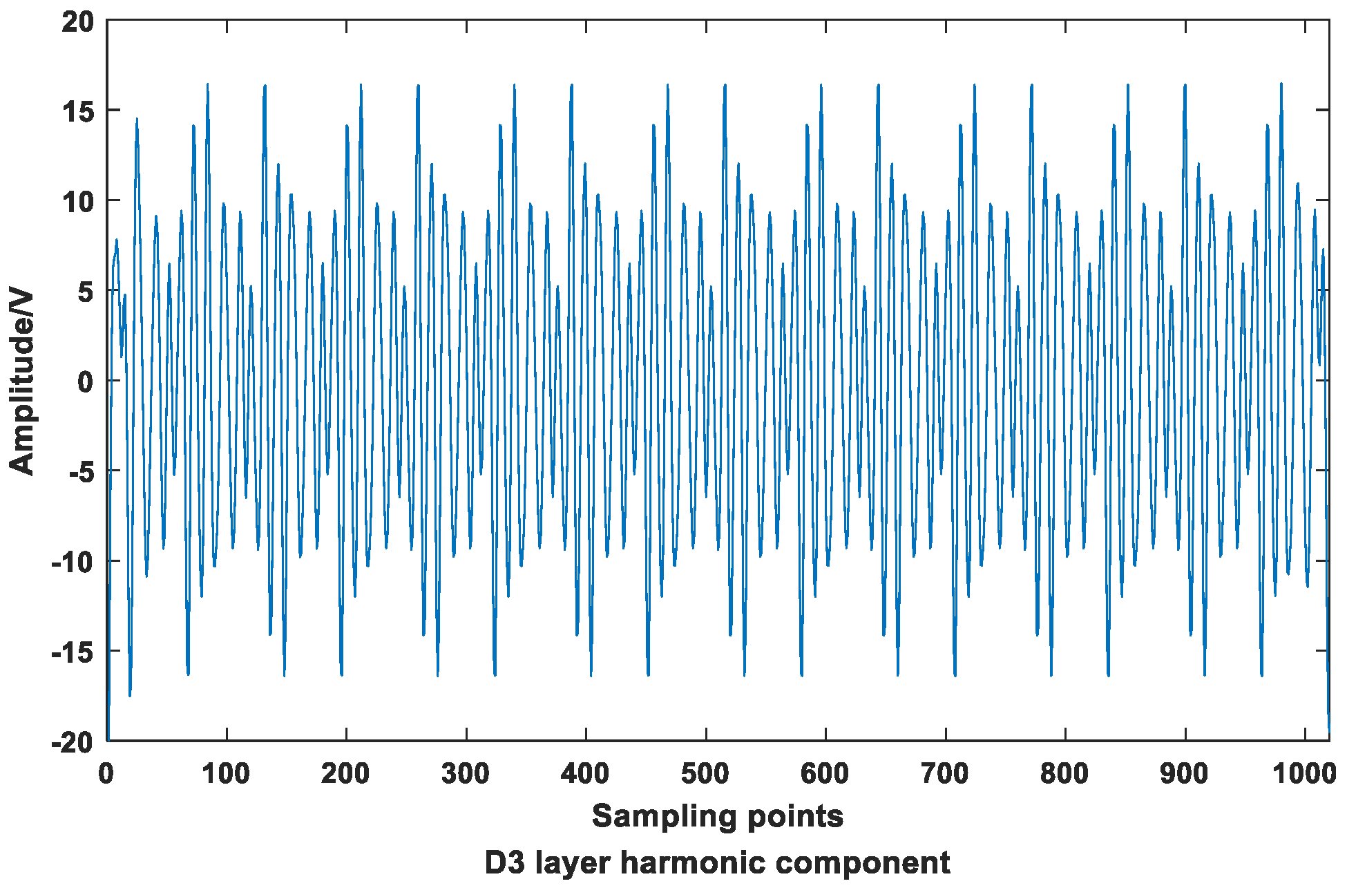
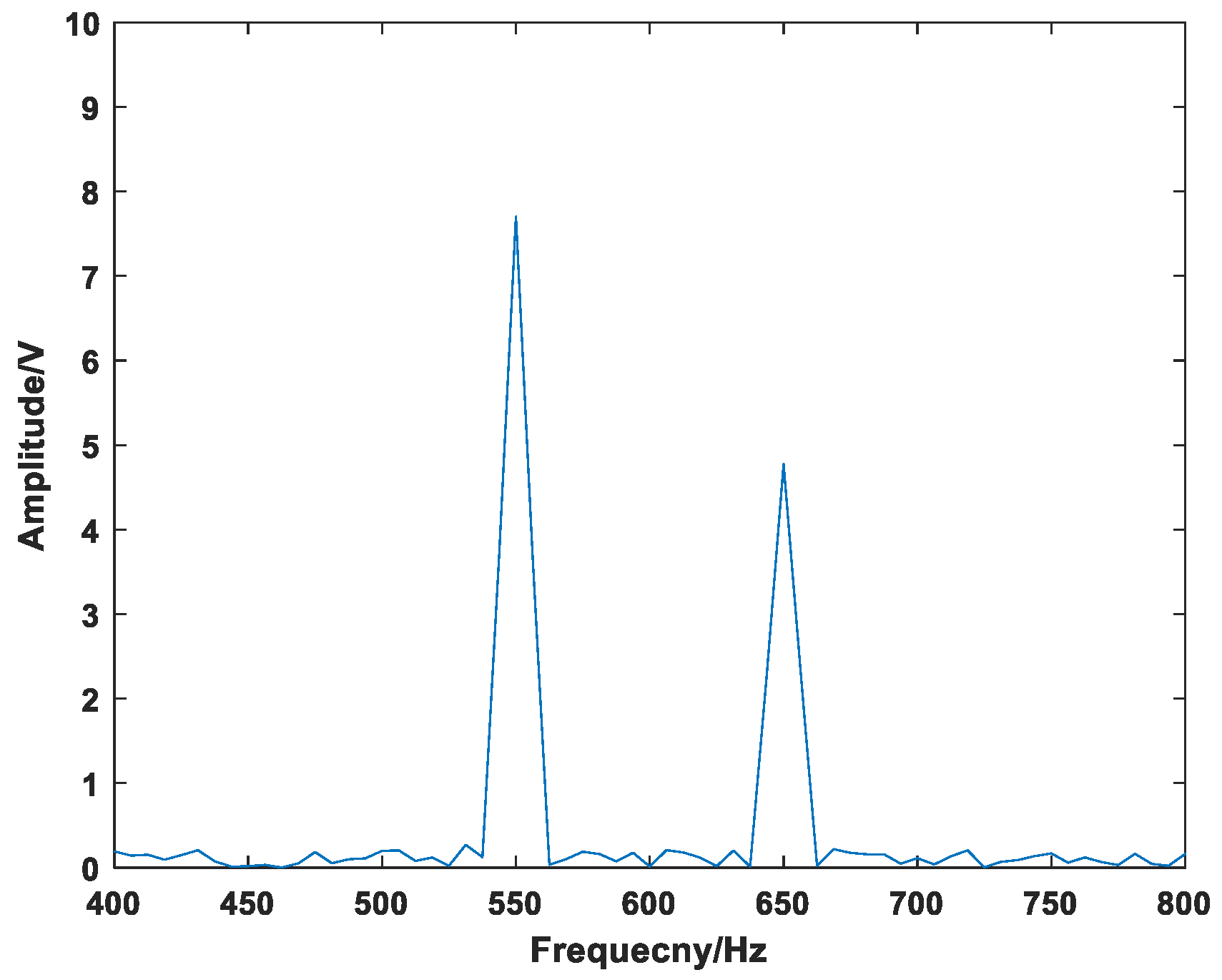
Decomposed by the Mallat algorithm, the frequency of the D3 layer is 400~800 Hz. According to the signal model, it can be seen that there are only the 11th and 13th harmonic components. The D3 layer reconstruction is shown in Figure 8.

Using the method designed in this paper, each peak is extracted and divided into two parts. After the average value is obtained, the two parts are subtracted to obtain the attenuation rate. The average value of the first half of the peak is equal to the average value of the latter part of the peak, so the attenuation rate is 0. It can be judged that the D3 layer only contains steady-state components, and parameters are extracted from the data after windowing DFT after the reconstructed signal, and the high frequency harmonic signals are restored. The waveform diagram is shown in Figure 9.

Based on the Hanning window function interpolation DFT and DWT mixed harmonic detection methods, the steady state components in the high frequency part cannot be restored, so the two methods cannot be compared. It can be seen from Figure 10 that the simulation result is very close to the theoretical value, and its specific data are shown in

Table 5. Analysis result table of high frequency steady-state harmonic component of D3 layer.

Number of Harmonic	Theory Frequency (Hz)	Actual Frequency (Hz)	Theory Amplitude (V)	Actual Amplitude (V)	Accuracy (%)
11	550	549.13	8	7.71	96.365
13	650	650.32	5	4.77	95.4

. The data obtained in the table are the average of three sets of data.

4.3.2. High Frequency Steady-State and Attenuation Component Simulation Results

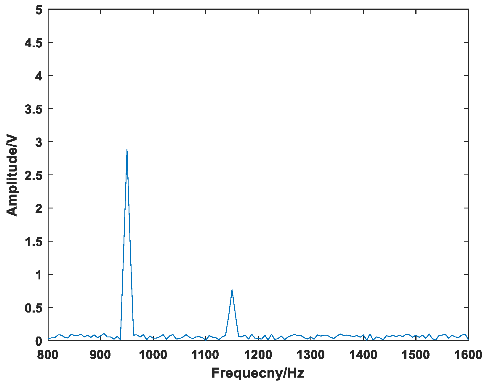
The frequency of the D2 layer is 800~1600 Hz, including the 19th and 23rd harmonics. The reconstruction of the D2 layer is shown in Figure 10.

In Figure 10, the attenuation trend of the waveform is not obvious. It can be known from the calculation of the attenuation rate that the second half is smaller than the first half, so there is an attenuation harmonic component in the D2 layer. To continue to determine whether it contains a steady-state component, perform DFT processing on the D2 layer, as shown in Figure 11.

In Figure 11, there are 19th and 23thharmonic components in the D2 layer, and the amplitude of the 19th harmonic component is 2.84 V. It can be determined that a steady-state harmonic component exists in the D2 layer. Because the DFT can only restore the waveform of the exponentially attenuated harmonic signal as a steady-state harmonic signal, and the amplitude is less than 50% of the actual amplitude; the amplitude of the 23th attenuation harmonic component is 0.77 V. For the steady-state components, the windowed interpolation DFT algorithm can better measure its key parameters, and the restored signal is basically consistent with the actual signal. For the attenuation component, the improved method uses the D2 layer data to subtract the steady-state component windowed and interpolated DFT data, leaving only the remaining attenuation component data as the reconstruction data for the attenuation harmonics. The reconstructed attenuation component is shown in Figure 12.

Using the reconstruction attenuation component and data of each harmonic extracted from the D2 layer, the recovered D2 layer waveform is compared with the original data. As shown in Figure 13, the error between the recovered data and the original data may be due to some sample values not being collected.

4.3.3. High Frequency Attenuation Component Simulation Results

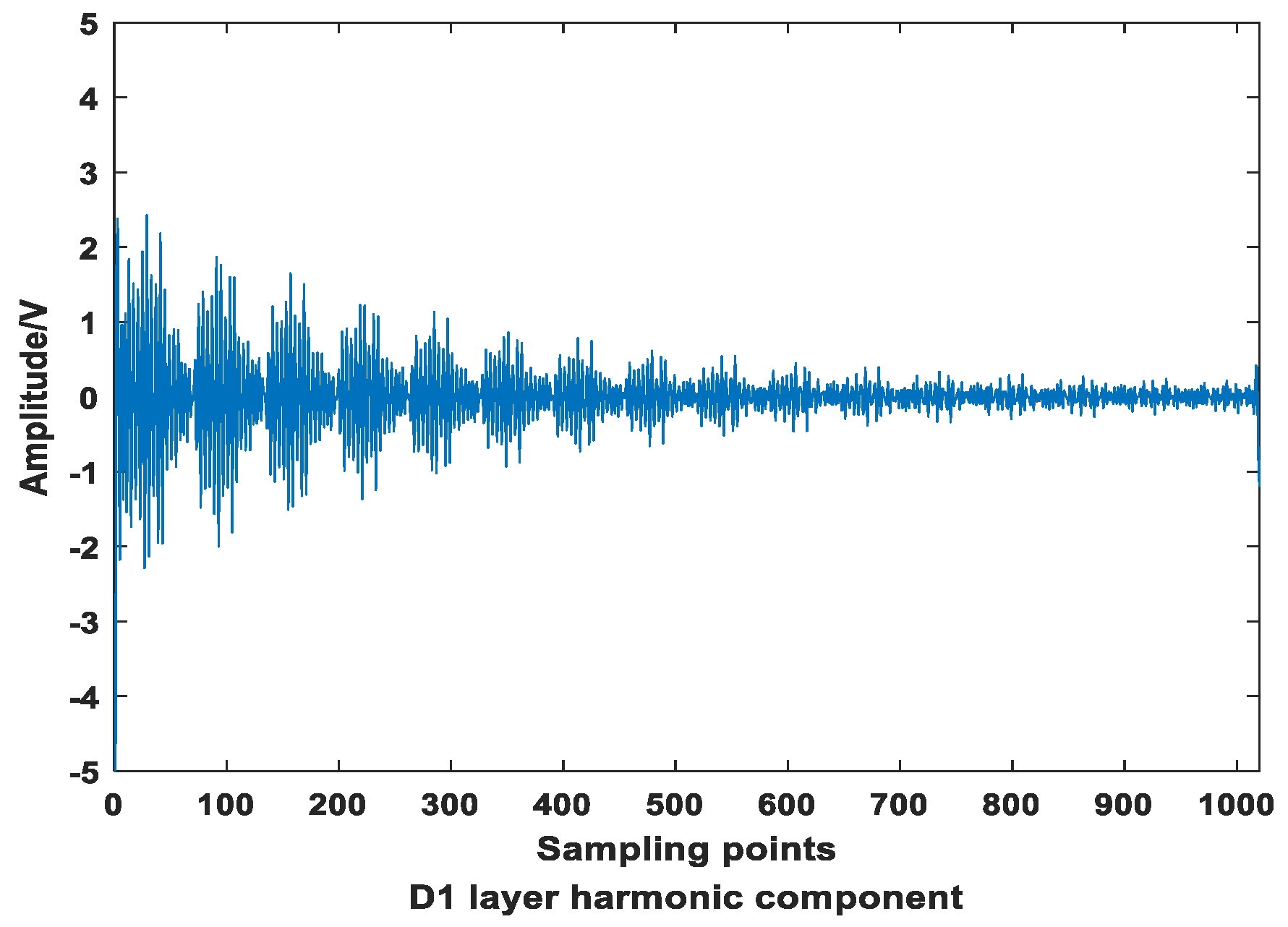
The frequency of the D1 layer is 1600~3200 Hz, including the 33th harmonic. The reconstruction of the D1 layer is shown in Figure 14.

Only the attenuation component exists in the high frequency part, and the 33th harmonic component can be directly restored by reconstructing the D1 layer. The maximum amplitude at the initial moment is about 10 V, and the waveform is attenuated approximately exponentially.

5. Conclusions

This paper designs a mixed harmonic detection method based on DFT and DWT using the Bartlett–Hann window function. The improved method realizes the separation and extraction of steady-state harmonics and attenuation harmonics in the high frequency part, which makes up for the shortcomings of the original method. The detection accuracy of the high frequency steady-state is about 95.9%. At the same time, the accuracy of the steady state harmonic detection in the low frequency part is guaranteed. The relative error between the detection accuracy and the theoretical value is less than 5%, and the accuracy is 95.3375%, which is 1.5175% higher than the existing method. Simulation results show that the harmonic detection method designed in this paper not only improves the detection accuracy, but also can more effectively detect and restore each harmonic component in the harmonic signal, which is helpful to improve the ability of harmonic analysis in the power grid. The method proposed in this paper can separate the steady-state harmonics from the high frequency non-steady-state part and can be applied to the analysis of complex harmonics in the power grid.

The data in this article illustrate the effectiveness and feasibility of the proposed method, not an absolute value. Applying the Monte Carlo simulation algorithm to improve and perfect the proposed method will give us a future research direction.

References

- Watson, N.R. Power-quality management in New Zealand. IEEE Trans. Power Deliv. 2016, 31, 1963–1970. [Google Scholar] [CrossRef]
- Reddy, M.J.B.; Sagar, K.; Mohanta, D.K. Multifunctional real-time power quality monitoring system using Stockwell transform. IET Sci. Meas. Technol. 2014, 8, 155–169. [Google Scholar] [CrossRef]
- Gao, Z.Q.; Zhao, H.J.; Zhou, X.S.; Ma, Y.J. Summary of power system harmonics. In Proceedings of the 29th Chinese Control and Decision Conference, Chongqing, China, 28–30 May 2017; pp. 2287–2291. [Google Scholar]
- Peng, Y.L.; Zhang, K.F.; Li, Y.B.; Yang, P.K.; Liu, H.Q. Improved harmonic detection algorithm applied to APF. In Proceedings of the IEEE 29th Chinese Control and Decision Conference, Chongqing, China, 28–30 May 2017; pp. 6948–6952. [Google Scholar]
- Subhamita, R.; Sudipta, D. ANN based method for power system harmonics estimation. In Proceeding of the IEEE Applied Signal Processing Conference, Kolkata, India, 7–9 December 2018; pp. 39–43. [Google Scholar]
- Wang, K.; Xie, F.; Zheng, C.B.; Hang, B. Research on harmonic detection method based on BP neural network used in induction motor controller. In Proceeding of the IEEE 12th Conference on Industrial Electronics and Applications, Siem Reap, Cambodia, 18–20 June 2017; pp. 578–582. [Google Scholar]
- Apetrei, V.; Filote, C.; Graur, A. Harmonic analysis based on discrete wavelet transform in electric power system. In Proceeding of the 9th International Conference on Ecological Vehicles and Renewable Energies, Monte-Carlo, Monaco, 25–27 March 2014. [Google Scholar]
- Wang, W.; Ma, X.P.; Wang, Q.J. Research on fault detection of wind turbine based on wavelet analysis. Int. J. Control Autom. 2015, 11, 127–134. [Google Scholar]
- Lai, Z.Q.; Xiao, Z.H.; Zhang, G.Q.; Wang, G.Z.; Liu, Y.; Chen, H.M.; Gao, X. Application of FFT interpolation correction algorithm based on window function in power harmonic analysis. In Proceeding of the 4th International Conference on Environmental Science and Material Application, Xian, China, 15–16 December 2018. [Google Scholar]
- Chen, J.; Wang, W.; Wang, S.H.; Yang, S.M. An approach for electrical harmonic FFT analysis based on Hanning self-multiply window. Power Syst. Prot. Control. 2016, 19, 114–121. [Google Scholar]
- Fang, G.Z.; Yang, C.; Zhao, H. Detection of harmonic in power system based on FFT and wavelet packet. Power Syst. Prot. Control. 2012, 5, 75–79. [Google Scholar]
- Zhu, X.; Xie, D.; Gao, Q.; Zhang, Y.C. Analysis strategy for power system harmonic based on FFT and DWT using db20. Power Syst. Prot. Control. 2012, 40, 62–66. [Google Scholar]
- Ha, Y.H.; Pearce, J.A. New window and comparison to standard windows. IEEE Trans. Acoust. Speech Signal Process. 1989, 37, 298–301. [Google Scholar] [CrossRef]
- Nath, S.; Sinha, P.; Goswami, S.K. A wavelet based novel method for the detection of harmonic sources in power systems. Int. J. Electr. Power Energy Syst. 2012, 40, 54–61. [Google Scholar] [CrossRef]
- Liu, H.; Ren, H.M.; Xiao, Z.H.; Zhao, T. Research on signal extrapolation in the time domain based on wavelet analysis. J. Eng. 2019, 20, 6533–6536. [Google Scholar] [CrossRef]
- Agarwal, P.; Singh, S.P.; Pandey, V.K. Spectrum shaping analysis using tunable parameter of fractional based on Bartlett window. In Proceeding of the 3rd IEEE International Advance Computing Conference, Ghaziabad, India, 22–23 February 2013; pp. 1625–1630. [Google Scholar]
- Tian, W.B.; Yu, J.M.; Ma, X.J.; Li, L. Power system harmonic detection based on Bartlett-Hann windowed FFT interpolation. In Proceedings of the Asia-Pacific Power and Energy Engineering Conference, Shanghai, China, 27–29 March 2012. [Google Scholar]
- Su, T.X.; Yang, M.F.; Jin, T.; Flesch, R.C.C. Power harmonic and interharmonic detection method in renewable power based on Nuttall double-window all-phase FFT algorithm. IET Renew. Power Gener. 2018, 12, 953–961. [Google Scholar] [CrossRef]
- Li, Z.H.; Hu, T.H.; Abu-Siada, A. A minimum side-lobe optimization window function and its application in harmonic detection of an electricity gird. Energies 2019, 12, 2619. [Google Scholar] [CrossRef] [Green Version]
- Wang, Z.J.; Qi, X.H.; Cai, J. Estimation of electrical harmonic parameters by using the Interpolated FFT algorithm based on Blackman window. J. Zhejiang Univ. 2006, 33, 650–653. [Google Scholar]
- Luo, C.H.; Xu, X.L.; An, M.Q.; Mao, L.K.; Zhou, W. Research and design of data acquisition and processing algorithm based on improved FFT. In Proceeding of the 31st Chinese Control and Decision Conference, Nanchang, China, 3–5 June 2019; pp. 1599–1604. [Google Scholar]
Figure 1.
Three-layer wavelet decomposition reconstruction diagram.
Figure 2.
Bartlett–Hann window spectrum comparison with several common windows.
Figure 3.
Harmonic detection improvement method flowchart.
Figure 4.
Waveform of complex harmonic signal .
Figure 5.
Low frequency coefficients and high frequency coefficients of the signal .
Figure 6.
Reconstructed waveform of A3 layer.
Figure 7.
A3 layer windowed interpolation DFT spectrum comparison chart.
Figure 8.
D3 layer reconstruction waveform.
Figure 9.
D3 layer high frequency steady-state spectrum.
Figure 10.
D2 layer reconstruction waveform.
Figure 11.
D2 layer DFT spectrum.
Figure 12.
D2 layer reconstruction attenuation component.
Figure 13.
D2 layer reconstruction waveform compared with the original waveform.
Figure 14.
D1 layer reconstructed waveform.