Cosmological Spectrum of Two-Point Correlation Function from Vacuum Fluctuation of Stringy Axion Field in De Sitter Space: A Study of the Role of Quantum Entanglement

Abstract

In this work, we study the impact of quantum entanglement on the two-point correlation function and the associated primordial power spectrum of mean square vacuum fluctuation in a bipartite quantum field theoretic system. The field theory that we consider is the effective theory of axion field arising from Type IIB string theory compacted to four dimensions. We compute the expression for the power spectrum of vacuum fluctuation in three different approaches, namely (1) field operator expansion (FOE) technique with the quantum entangled state, (2) reduced density matrix (RDM) formalism with mixed quantum state and (3) the method of non-entangled state (NES). For a massless axion field, in all three formalisms, we reproduce, at the leading order, the exact scale invariant power spectrum which is well known in the literature. We observe that due to quantum entanglement, the sub-leading terms for these thee formalisms are different. Thus, such correction terms break the degeneracy among the analysis of the FOE, RDM and NES formalisms in the super-horizon limit. On the other hand, for massive axion field we get a slight deviation from scale invariance and exactly quantify the spectral tilt of the power spectrum in small scales. Apart from that, for massless and massive axion field, we find distinguishable features of the power spectrum for the FOE, RDM, and NES on the large scales, which is the result of quantum entanglement. We also find that such large-scale effects are comparable to or greater than the curvature radius of the de Sitter space. Most importantly, in near future if experiments probe for early universe phenomena, one can detect such small quantum effects. In such a scenario, it is possible to test the implications of quantum entanglement in primordial cosmology.

1. Introduction

The concept of quantum entanglement is one of the most interesting features that one can study in the context of quantum mechanics. Using such an idea, one can study the instantaneous physical implication of local measurements [1,2,3]. There are several applications in the framework of quantum field theory in which the quantum entanglement play a significant role. For example, particle creation (EPR Bell pair [4]) through the bubble nucleation procedure was explained using the idea of quantum entanglement where the quantum system is strongly correlated [5,6,7,8,9]. Also using the concept of quantum entanglement in QFT one successfully explains many phenomena such as entropy bounds, phase transitions, anomalies, confinement, thermalization and quantum critical quenches, localization in quantum gravity and description of interior of black holes. Apart from that quantum entanglement has huge application in the context of quantum information theory, quantum cryptography and interferometry.

The von-Neumann entropy and R$\acute{e}$nyi entropy are the appropriate measures of quantum entanglement the framework of condensed matter theory [10], in quantum information theory and in theoretical high energy physics. The idea of entanglement entropy in the context of quantum field theory is the best possible computational tool to quantify and study the nature of the long range effects of quantum correlation. However, the computation of entanglement entropy for a specific class of quantum field theories were not easy before the method proposed by Ryu and Takayanagi [11]. In this work, the authors have computed the entanglement entropy for a strongly coupled field theory set up with a gravity dual using the techniques of holography and the results are remarkable as it is in agreement with various expectations from the quantum field theory side [11,12,13,14,15,16].

Following this success, Maldacena and Pimentel in ref. [17] further proposed an explicit technique to compute the entanglement entropy in the framework of quantum field theory of de Sitter space with Bunch Davies quantum initial vacuum state1. It is important to note in particular that the Green functions which verify a condition (commonly known as the Hadamard condition) behave on the light-cone as in flat space for Bunch Davies or the Euclidean false vacuum state. On the other hand, the Bunch Davies or the Euclidean false vacuum can also be physically interpreted as being generated by an infinite time tracing operation from the condition that the energy scale of the quantum mechanical fluctuations is much smaller than the characteristic scale in cosmology, which is the Hubble scale. This quantum vacuum state possesses actually no quanta at the limiting asymptotic past infinity. However, in the framework of quantum field theory of curved space time, there exists a huge class of quantum mechanical vacuum states in the background De Sitter space time which are invariant under all the $SO(1,4)$ isometries and commonly known as the $\alpha$-vacua. Here $\alpha$ is a real parameter which forms a real parameter family of continuous numbers to describe the issometric classes of invariant quantum vacuum state in De Sitter space. In a more technical sense, sometimes the $\alpha$ vacua is characterized as the squeezed quantum vacuum state in the context of quantum field theory of curved space time. It is also important to note that in the original version something called, $\alpha ,\beta$ or Motta-Allen (MA) vacua is appearing which is CPT violating and here an additional real parameter $\beta$ is appearing in the phases in the definition of the quantum mechanical vacuum state. This phase factor is responsible for the CPT violation. Once we switch off this phase factor by fixing $\beta =0$, the one can get back the CPT symmetry preserving quantum vacuum state in the present context. The $\alpha$ vacua and the Bunch Davies or Euclidean false vacuum are connected to each other via Bogoliubov transformation. Especially, the $\alpha =0$ case corresponds to the Bunch Davies or Euclidean vacuum state in which the Hadamard condition in the Green’s functions is satisfied. Additionally, the point to be noted here that the Bunch-Davies or the Euclidean quantum vacuum state is actually representing a zero-particle quantum mechanical state which is observed by a geodesic observer, which implies that an observer who is in free fall in the expanding state is characterized by this vacuum state. Because of this reason to explain the origin of quantum mechanical fluctuations appearing in the context of cosmological perturbation theory in the inflationary models or during the particle production phenomena the concept of Euclidean false quantum vacuum state is commonly used in primordial cosmology literature. Here, the authors have studied the gravitational dual of the quantum field theory of De Sitter space using holographic techniques in detail. Furthermore, in ref. [18] the authors have extended this computation in the context of $\alpha$ vacua [19,20,21,22] in the same context. In ref. [23,24] the computation of quantum entanglement entropy and the formation of EPR Bell pair from stringy Axion2 were discussed with Bunch Davies and $\alpha$ vacua respectively.

Based on the physical set up used in our previous works [23,24], in this paper we studied the cosmological implications of quantum entanglement by focussing on the long range effects of the two point correlation function computed from the mean square vacuum fluctuation of stringy Axion field with Bunch Davies and $\alpha$ quantum states as initial choice of vacua. We expect from this analysis that the signature and impact of quantum entanglement could be manifest in the correlation function even beyond the Hubble horizon scale. Our expectation is mainly due to the fact that de Sitter expansion of universe distinguish between a pair of Axions [27,28,29,30], known as EPR Bell pair which is created within causally connected Hubble region. For this purpose, we use three different techniques:

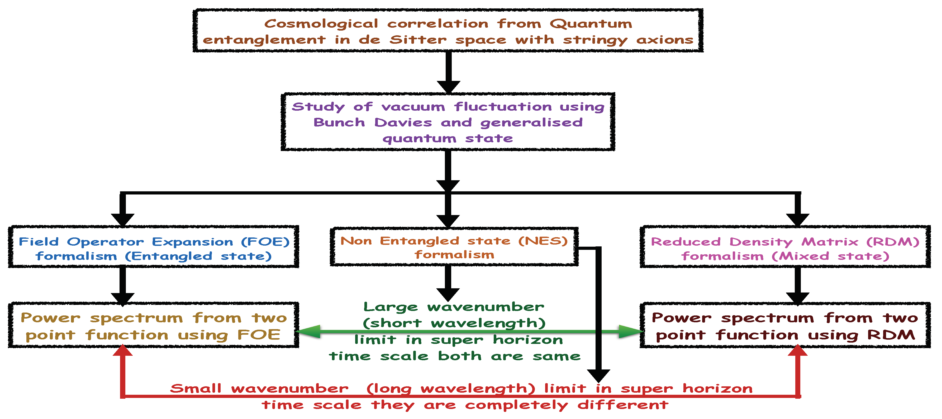
• Field operator expansion (FOE) method with entangled state,
• Reduced density matrix formalism (RDM) with mixed state and
• Non-entangled state (NES) method.

Here one can ask the following sets of questions regarding the implementation of three different techniques in the present context:

• Q1. Why did we use three different formalisms to compute the cosmological two point correlation function?
• Q2. What is the correct physics they believe that happens in the setup of the space time?
• Q3. In those three formalisms, the physics is completely different. So which one is correct?
• Q4. We finally could only observe one possible observational consequence. So which one is correct?

The appropriate answers to above mentioned questions are appended below point wise:

• A1. We used three different formalisms to compute the cosmological two point correlation function to check the explicit role of quantum mechanical entanglement in the primordial cosmology. In these three formalisms the leading order expressions become same. However, the difference only can be found once we look into the small quantum corrections appearing in these formalisms. If the signature of quantum entanglement will be detected in near future in the observational probes of early universe, then one can explicitly rule out the possibility of appearing of NES method in the context of quantum field theory of primordial cosmology. On the other hand, if the signatures of quantum entanglement cannot be confirmed then one can strongly rely on the result obtained in the NES method. Additionally, it is important to note that these three frameworks provide us the quantum mechanical origin of quantum field theory of early universe cosmology.
• A2 and A3. From the theoretical perspective these three different formalisms have their own merit on the physical ground. If the quantum mechanical origin of the quantum correction of the primordial fluctuation is coming from the non entangled state then NES formalism is the only single option which can take care of the correct physics. On the other hand, if the quantum mechanical origin of the quantum correction of the primordial fluctuation is coming from the entangled mixed state then RDM formalism applicable to the subsystem is the most promising option which supports correct physical explanation. The last option is FOE formalism which is applicable when the quantum mechanical origin of the quantum correction of the primordial fluctuation is guided by the total entangled state (not the subsystem) then FOE formalism is useful to describe the correct physics.
• A4. It is very well known fact that at late time scale all the large scale structure is formed due to long range persistent correlation originated from the primordial quantum mechanical fluctuation in the early universe. This can only be consistently theoretically established by using FOE and RDM formalisms which supports the concept of quantum entanglement in early universe cosmology. Now RDM formalism is more theoretically consistent than the FOE method as it is based on the quantum description of the reduced subsystem. Now as far as the detection in the observation is concerned, if we can detect the quantum mechanical origin of the sub leading quantum correction in near future probes then one can explicitly very the explicit role of quantum entanglement, precisely test FOE or RDM formalism is correct. If we cannot detect the role of quantum entanglement then NES formalism will provide the correct physical explanation of the quantum origin of the sub leading correction term in the two point primordial correlation function.

We implement the RDM formalism using the previous work done by Maldacena and Pimentel in ref. [17] in the context of de Sitter cosmology. In our computation we explicitly included the effect of Stringy Axion in the small field regime and as a result we get perturbatively corrected contributions in the expression for the power spectrum derived using FOE, RDM and NES formalisms. Such correction terms can be interpreted as quantum effects which are appearing from the UV complete theory, such as a specific type of bipartite quantum field theory driven by axion. We note that the axion field which is being considered here, is actually originating from Type IIB string theory compactified on a Calabi-Yau three fold (${\mathbf{CY}}^{\mathbf{3}}$), in presence of a $\mathbf{NS}\mathbf{5}$ brane sitting at the bottom of a long throat [31,32,33,34]. Most importantly, in the large wave number3 limit (small scale or small wave length approximation [35]) we showed the results for the power spectrum derived from these three formalism perfectly match with each other if we consider only the leading order contribution. However, the results are different for these three formalisms if we we include the contributions from next and next to next leading order. In a way one can say that such additional small perturbative correction terms play a pivotal role to distinguish between the FOE, RDM and NES formalisms. This is obviously an important information because using the present observational data on early universe cosmology [36,37,38,39,40,41,42,43,44,45,46,47,48,49,50,51,52,53,54,55,56,57,58,59,60,61,62,63,64,65,66,67,68,69,70,71,72,73,74,75,76,77,78,79,80,81,82,83,84,85,86,87,88,89,90,91,92,93,94] one can further constrain the present model and also test the appropriateness of these formalisms. Apart from this, for completeness, we also analysed the behaviour of the power spectrum in the small wave number limit (large scale or large wave length approximation). We find that all these three formalisms yield distinctive results in terms of the momentum (quantum number) dependence of the power spectrum in order by order. However, the lack of observational data on this particular regime does not allow us to test the appropriateness and correctness of the proposed methods. We hope that in near future when the observational data for this regime will be available, our results can further constrain the model and rule out two of the possibilities between the three formalisms discussed here. We would like to mention here that in our computation of the power spectrum for mean square vacuum fluctuation we have not considered the quantum fluctuation of the pseudo scalar Axion field as a classical back ground field, the approach which is mostly used in the context of the cosmological correlations from early universe. Instead, we chosen the field operator of the Axion field itself as quantum operator whose fluctuation with respect to a quantum mechanical vacuum state (Bunch Davies and $\alpha$ vacua). Thus, in this paper, we followed:

• A complete quantum approach to compute the primordial power spectrum of mean square vacuum fluctuation, which is not usually followed in the context of cosmology.
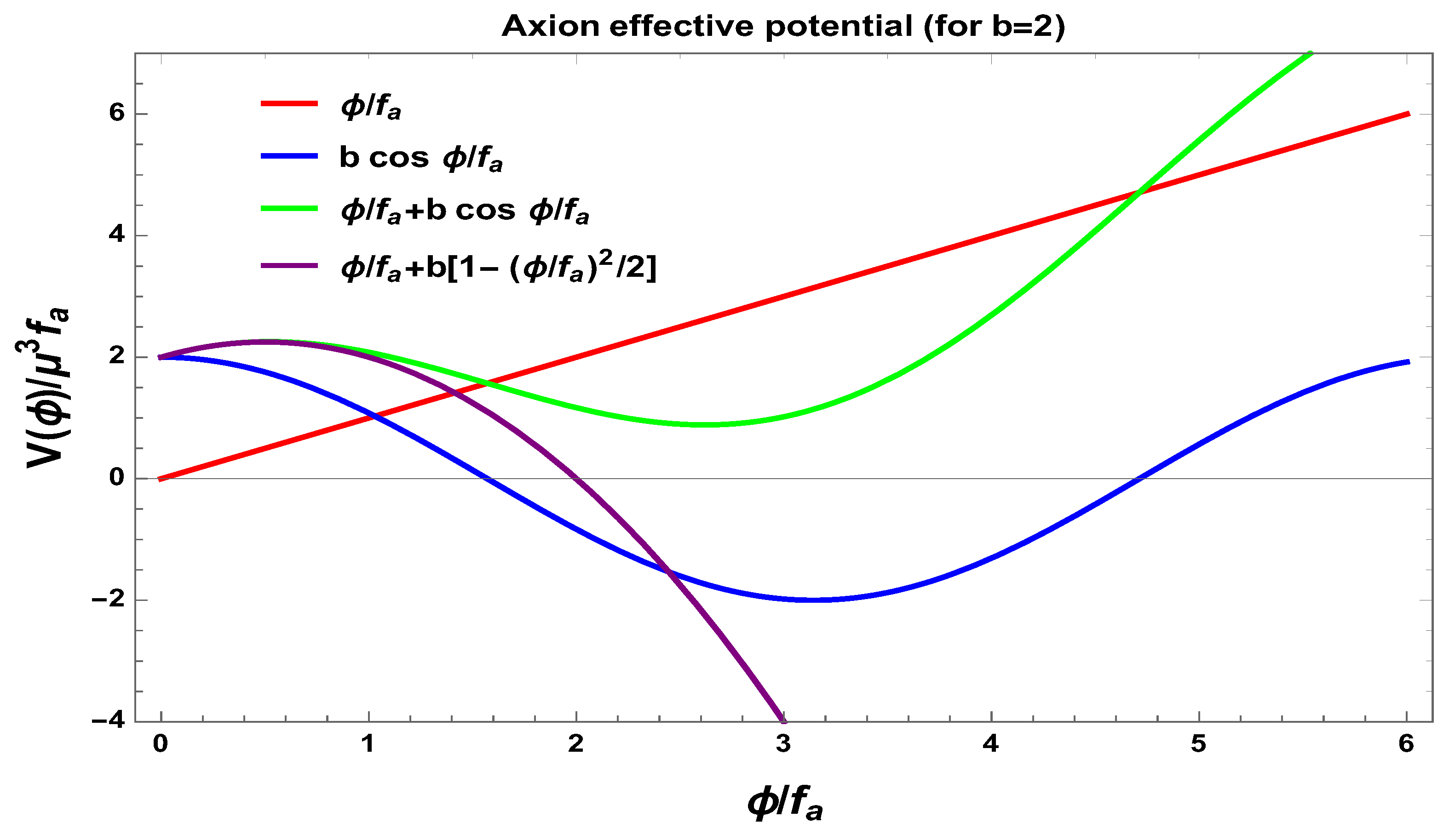
• For the specific structure of the axion effective potential, we computed the explicit form of the corrections which are due to quantum effects.
• For our calculation, we used three different approaches at super horizon time scale hoping that the quantum corrections, at small and large wave number limits when confronted with observations, can select the most effective approach and the nature of quantum corrections. From the cosmological perspective we believe this is a very important step forward.

The plan of the paper is as follows: In Section 2, we begin our discussion with the computation of the wave function of the Axion field in a de Sitter hyperbolic open chart. For this purpose, we discuss the details of the background de Sitter geometrical set up in Section 2.1. Furthermore, in Section 2.2 and Section 2.3, we solve the total wave function for Axion for Bunch Davies vacuum and generalised $\alpha$- vacua respectively. Using these solutions we derived the cosmological power spectrum of mean square quantum vacuum fluctuation in Section 3. In Section 3.1.1 and Section 3.1.2 we discuss the quantum vacuum fluctuation using field operator expansion (FOE) formalism with entangled state for Axion. field. We also derived the explicit form of the wave function in this formalism. This solution is used to derive the power spectrum by computing the two point quantum correlation function from mean square vacuum fluctuation. In Section 3.2.1and Section 3.2.2 we discuss the quantum vacuum fluctuation using reduced density matrix (RDM) formalism using mixed state for Axion field and we derived the explicit form of the reduced density matrix in the de Sitter hyperbolic open chart. Furthermore, this result is used to derive the power spectrum by computing the two point quantum correlation function from mean square vacuum fluctuation in large and small wave number limits for both massless and massve Axion fields. In Section 3.3.1and Section 3.3.2 we study the quantum vacuum fluctuation using non entangled state (NES) formalism for Axion field and have discussed the NES formalism in detail. This result was used to derive the power spectrum by computing the two point quantum correlation function from mean square vacuum fluctuation. Finally, Section 4 is devoted to a summary, conclusions and future prospects. In Figure 1, we present a schematic diagram for the computation algorithm of long range effect of cosmological correlation function from quantum entanglement of axion in de Sitter open hyperbolic chart.

2. Wave Function of Axion in Open Chart

We briefly review here, for the sake of completeness, the background geometry and the results for wave function of the axion field.

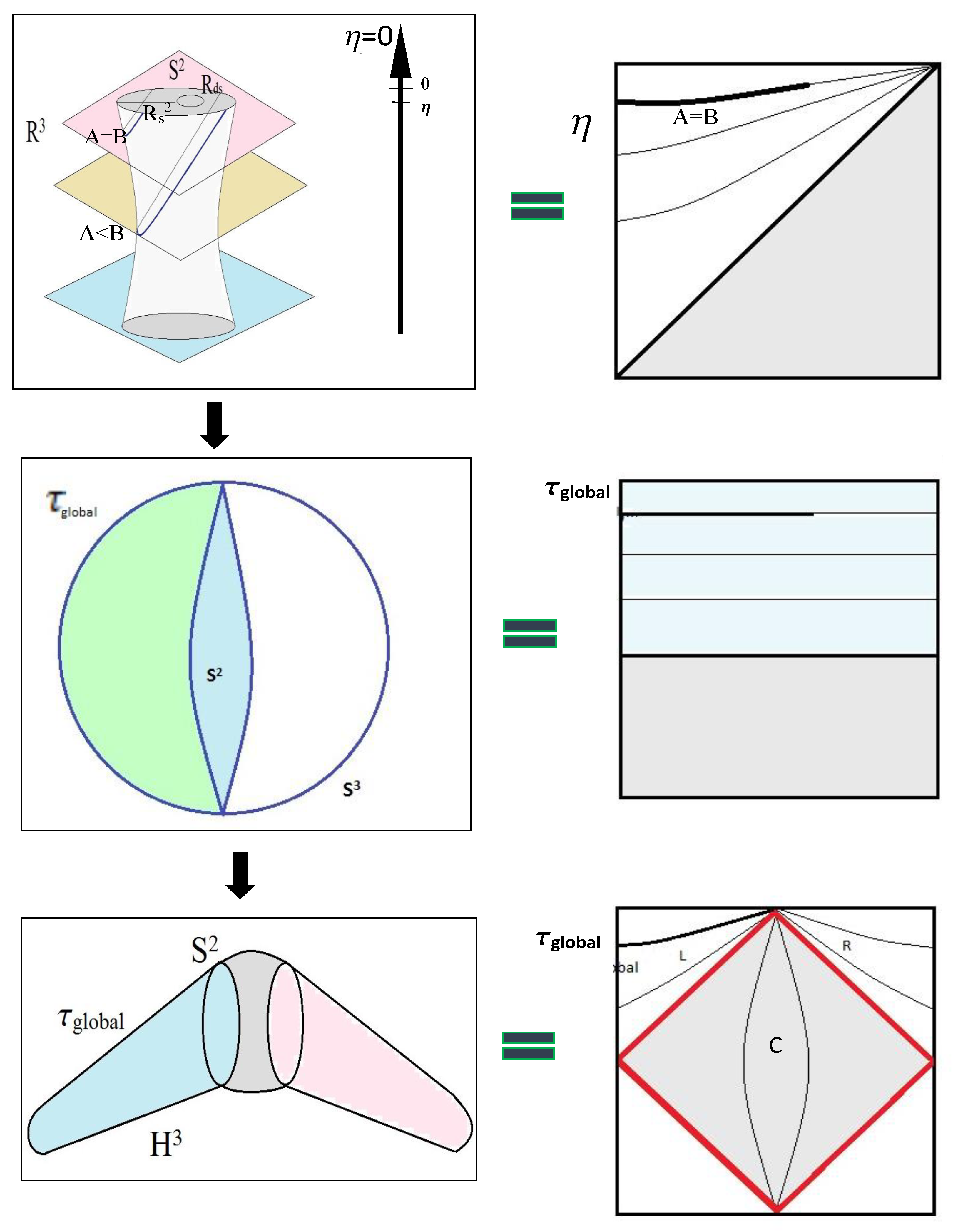
2.1. Background Geometry

We consider a time preserving space-like hypersurface ${\mathbf{S}}^{\mathbf{2}}$ in the open hyperbolic chart of the de Sitter space. As a result, ${\mathbf{S}}^{\mathbf{2}}$ is divided into two sub regions-interior and exterior which are identified by RI (≡ L)/RII (≡ R). In terms of the Lorentzian signature an open chart in de Sitter space is described by three different subregions:

$$\begin{array}{ccc}\hfill {\displaystyle \mathbf{R}(=\mathbf{RII})/\mathbf{L}(=\mathbf{RI})}& :& {\displaystyle \left\{\begin{array}{cc}{\displaystyle {\tau }_{\mathrm{E}}=\pm \frac{\pi }{2}\mp i{t}_{\mathbf{R}/\mathbf{L}}}\hfill & t_{\mathbf{R}}\ge \mathbf{0}/t_{\mathbf{L}}\ge \mathbf{0}\hfill \\ {\displaystyle {\rho }_{\mathrm{E}}=-i{r}_{\mathbf{R}/\mathbf{L}}}\hfill & r_{\mathbf{R}}\ge \mathbf{0}/r_{\mathbf{L}}\ge \mathbf{0}\hfill \\ {\displaystyle d{s}_{\mathbf{R}/\mathbf{L}}^2=\frac{1}{H^2}\left[-d{t}_{\mathbf{R}/\mathbf{L}}^2+{sinh}^2{t}_{\mathbf{R}/\mathbf{L}}\left(d{r}_{\mathbf{R}/\mathbf{L}}^2+{sinh}^2{r}_{\mathbf{R}//\mathbf{L}}d{\mathsf{\Omega }}_{\mathbf{2}}^2\right)\right]}\hfill \end{array}\right.}\hfill \end{array}$$

(1)

$$\begin{array}{ccc}\hfill {\displaystyle \mathbf{C}}& :& {\displaystyle \left\{\begin{array}{cc}{\displaystyle {\tau }_{\mathrm{E}}=t_{\mathbf{C}}}\hfill & -\frac{\pi }{\mathbf{2}}\le t_{\mathbf{C}}\le \frac{\pi }{\mathbf{2}}\hfill \\ {\displaystyle {\rho }_{\mathrm{E}}=\frac{\pi }{2}-i{r}_{\mathbf{C}}}\hfill & -\infty <r_{\mathbf{c}}<\infty .\hfill \\ {\displaystyle d{s}_{\mathbf{C}}^2=\frac{1}{H^2}\left[d{t}_{\mathbf{C}}^2+{cos}^2{t}_{\mathbf{C}}\left(-d{r}_{\mathbf{C}}^2+{cosh}^2{r}_{\mathbf{C}}d{\mathsf{\Omega }}_{\mathbf{2}}^2\right)\right]}\hfill \end{array}\right.}\hfill \end{array}$$

(2)

where $H=\dot{a}/a$ is the Hubble parameter and $d{\mathsf{\Omega }}_{\mathbf{2}}^2$ represents angular part of the metric on ${\mathbf{S}}^2$. Now let us assume that the total Hilbert space of the local quantum mechanical system is described by $\mathcal{H}$, which can be written using bipartite decomposition in a direct product space as, $\mathcal{H}={\mathcal{H}}_{\mathbf{INT}}\otimes {\mathcal{H}}_{\mathbf{EXT}}$. Here ${\mathcal{H}}_{\mathbf{INT}}$ and ${\mathcal{H}}_{\mathbf{EXT}}$ are the Hilbert space associated with interior and exterior region and describe the localised modes in RI/RII respectively.

In Figure 2 we show the schematic diagram for the geometrical construction and underlying symmetries of the bipartite quantum field theoretic system of de Sitter hyperbolic open chart. Corresponding Penrose diagrams are also drawn for completeness.

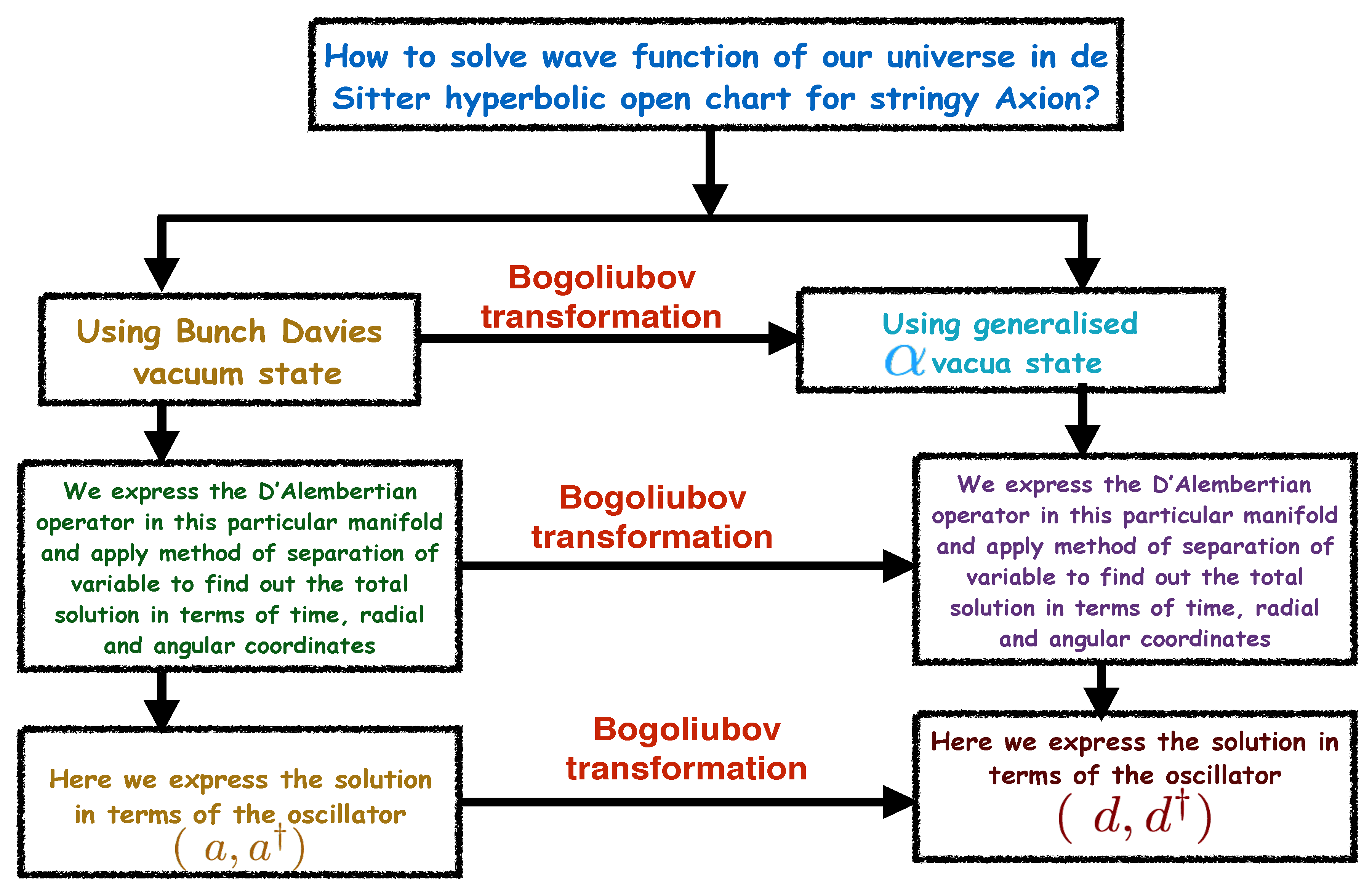
2.2. Wave Function for Axion Using Bunch Davies Vacuum

Though our prime objective is to compute the cosmological correlation functions for axion field in de Sitter space, we need the results for the wave function of the axion field in the just mentioned geometrical set up. Please note that the axion field under consideration is coming from RR sector of Type IIB string theory compactified on ${\mathbf{CY}}^{\mathbf{3}}$ in presence of $\mathbf{NS}\mathbf{5}$ brane [31,95]. The effective action for the axion field is given by [31]:

$$\begin{array}{ccc}\hfill S_{axion}& =& \int d^{4}x\sqrt{-g}\left[-\frac{1}{2}{(\partial \varphi )}^2+{\mu }^3\left\{\varphi +b{f}_{a}cos\left(\frac{\varphi }{f_a}\right)\right\}\right],\hfill \end{array}$$

(3)

where ${\mu }^3$ is the mass scale, $f_a$ is axion decay constant and the parameter b is defined as, $b={\mathsf{\Lambda }}_G^4/{\mu }^3{f}_a.$ Here ${\mathsf{\Lambda }}_G$ depend on the string coupling $g_s$, slope parameter ${\alpha }^{{}^{\prime }}$ and details of SUSY breaking parameter. For $\varphi <<f_a$, effective potential for axion can be expressed as:

$$\begin{array}{ccc}\hfill V\left(\varphi \right)& \approx & {\mu }^3\left(b{f}_a+\varphi \right)-\frac{m_{axion}^2}{2}{\varphi }^2,\hfill \end{array}$$

(4)

where we introduce the effective mass of the axion as, $m_{axion}^2={\mu }^{3}b/f_a={\mathsf{\Lambda }}_G^4/f_a^2.$ Here axion decay constant follow a (conformal) time dependent profile, which is explicitly mentioned in refs. [27,28,29].

In Figure 3 we explicitly present the behaviour of the above axion potential with respect to the dimensionless field value $\varphi /f_a$.

Furthermore, using Equation (3) the field equation of motion for the axion can be written as:

$$\begin{array}{ccc}\hfill \left[\frac{1}{a^3\left(t\right)}{\partial }_t\left(a^3\left(t\right){\partial }_t\right)-\frac{1}{H^2{a}^2\left(t\right)}{\widetilde{{\mathbf{L}}^{\mathbf{2}}}}_{{\mathbf{H}}^{\mathbf{3}}}+m_{axion}^2\right]\varphi & =& {\mu }^3,\hfill \end{array}$$

(5)

where the scale factor $a\left(t\right)$ in de Sitter open chart is given by, $a\left(t\right)=sinht/H$ and H is the Hubble parameter, which is in principle can be time-dependent. However, in the global patch of De Sitter space, it appears that the Hubble parameter H can be treated as approximately a constant throughout the evolutionary time scale of our universe and the value is fixed at very high energy scale, ${10}^{16}$ GeV at which the inflation and cosmological particle production (in the present context axion production) at very early universe are occurring. This value of the Hubble parameter is appearing from the observational constraint from Planck 2018 on the tensor-to-scalar ratio, which is actually a very important quantity in cosmology and determines the existence of primordial gravitational wave fluctuations at the very early time scale of our universe.

Additionally, it is important to note that the Laplacian operator ${\widetilde{{\mathbf{L}}^{\mathbf{2}}}}_{{\mathbf{H}}^{\mathbf{3}}}$, which is defined in the ${\mathbf{H}}^{\mathbf{3}}$ geometry can be written as:

$$\begin{array}{ccc}\hfill {\widetilde{{\mathbf{L}}^{\mathbf{2}}}}_{{\mathbf{H}}^{\mathbf{3}}}& =& \frac{1}{{sinh}^{2}r}\left[{\partial }_r\left({sinh}^{2}r{\partial }_r\right)+\frac{1}{sin\theta }{\partial }_{\theta }\left(sin\theta {\partial }_{\theta }\right)+\frac{1}{{sin}^2\theta }{\partial }_{\varphi }^2\right],\hfill \end{array}$$

(6)

which satisfy the following eigenvalue equation:

$$\begin{array}{ccc}\hfill {\widetilde{{\mathbf{L}}^{\mathbf{2}}}}_{{\mathbf{H}}^{\mathbf{3}}}{\mathcal{Y}}_{plm}(r,\theta ,\varphi )& =& -(1+p^2){\mathcal{Y}}_{plm}(r,\theta ,\varphi ).\hfill \end{array}$$

(7)

Here ${\mathcal{Y}}_{plm}(r,\theta ,\varphi )$ represents orthonormal eigenfunctions which can be written in terms of a radial and angular part as:

$$\begin{array}{ccc}\hfill {\mathcal{Y}}_{plm}(r,\theta ,\varphi )& =& \frac{\Gamma \left(ip+l+1\right)}{\Gamma \left(ip+1\right)}\frac{p}{\sqrt{sinhr}}{\mathcal{P}}_{\left(ip-\frac{1}{2}\right)}^{-\left(l+\frac{1}{2}\right)}\left(coshr\right)Y_{lm}(\theta ,\varphi ),\hfill \end{array}$$

(8)

where $Y_{lm}(\theta ,\varphi )$ is the spherical harmonics. Consequently, the total solution of the equations of motion can be written as:

$$\begin{array}{ccc}\hfill \mathsf{\Phi }(t,r,\theta ,\varphi )& =& \sum _{\sigma =\pm 1}\sum _{Q=p,l,m}\left[a_Q{\mathcal{V}}_Q(t,r,\theta ,\varphi )+a_Q^{†}{\mathcal{V}}_Q^{*}(t,r,\theta ,\varphi )\right],\hfill \end{array}$$

(9)

Here the total solution ${\mathcal{V}}_Q(t,r,\theta ,\varphi )$ for Bunch Davies vacuum can be expressed as:

$$\begin{array}{ccc}\hfill {\mathcal{V}}_Q(t,r,\theta ,\varphi )& =& \frac{1}{a\left(t\right)}{\chi }_{p,\sigma }\left(t\right){\mathcal{Y}}_{plm}(r,\theta ,\varphi )=\frac{H}{sinht}{\chi }_{p,\sigma }\left(t\right){\mathcal{Y}}_{plm}(r,\theta ,\varphi ),\hfill \end{array}$$

(10)

where ${\chi }_{p,\sigma }\left(t\right)$ forms a complete set of positive frequency function. Also this can be written as a sum of complementary (${\chi }_{p,\sigma }^{\left(c\right)}\left(t\right)$) and particular integral (${\chi }_{p,\sigma }^{\left(p\right)}\left(t\right)$) part, as given by:

$$\begin{array}{ccc}\hfill {\chi }_{p,\sigma }\left(t\right)& =& {\chi }_{p,\sigma }^{\left(c\right)}\left(t\right)+{\chi }_{p,\sigma }^{\left(p\right)}\left(t\right).\hfill \end{array}$$

(11)

Explicitly the solution for the complementary part and the particular integral part can be expressed as:

$$\begin{array}{ccc}\hfill {\displaystyle {\chi }_{p,\sigma }^{\left(c\right)}\left(t\right)}& =& {\displaystyle \left\{\begin{array}{cc}{\displaystyle \frac{1}{2sinh\pi p}\left[\frac{\left(e^{\pi p}-i\sigma e^{-i\pi \nu }\right)}{\Gamma \left(\nu +\frac{1}{2}+ip\right)}{\mathcal{P}}_{\left(\nu -\frac{1}{2}\right)}^{ip}(cosh{t}_{\mathbf{R}})-\frac{\left(e^{-\pi p}-i\sigma e^{-i\pi \nu }\right)}{\Gamma \left(\nu +\frac{1}{2}-ip\right)}{\mathcal{P}}_{\left(\nu -\frac{1}{2}\right)}^{-ip}(cosh{t}_{\mathbf{R}})\right]}\hfill & \mathbf{for}\mathbf{R}\hfill \\ {\displaystyle \frac{\sigma }{2sinh\pi p}\left[\frac{\left(e^{\pi p}-i\sigma e^{-i\pi \nu }\right)}{\Gamma \left(\nu +\frac{1}{2}+ip\right)}{\mathcal{P}}_{\left(\nu -\frac{1}{2}\right)}^{ip}(cosh{t}_{\mathbf{L}})-\frac{\left(e^{-\pi p}-i\sigma e^{-i\pi \nu }\right)}{\Gamma \left(\nu +\frac{1}{2}-ip\right)}{\mathcal{P}}_{\left(\nu -\frac{1}{2}\right)}^{-ip}(cosh{t}_{\mathbf{L}})\right]}\hfill & \mathbf{for}\mathbf{L},\hfill \end{array}\right.}\hfill \end{array}$$

(12)

$$\begin{array}{ccc}\hfill {\chi }_{p,\sigma }^{\left(p\right)}\left(t\right)& =& {sinh}^{2}t\sum _{n=0}^{\infty }\frac{1}{\left(p^2-p_n^2\right)}{\chi }_{p_n,\sigma }^{\left(c\right)}\left(t\right)\int d{t}^{{}^{\prime }}{\chi }_{p_n,\sigma }^{\left(c\right)}\left(t^{{}^{\prime }}\right){\mu }^3.\hfill \end{array}$$

(13)

where the parameter $\nu$ is defined as:

$$\begin{array}{ccc}\hfill \nu & =& \sqrt{\frac{9}{4}-\frac{m_{axion}^2}{H^2}}=\sqrt{\frac{9}{4}-\frac{{\mu }^{3}b}{f_a{H}^2}}=\sqrt{\frac{9}{4}-\frac{{\mathsf{\Lambda }}_G^4}{f_a^2{H}^2}}.\hfill \end{array}$$

(14)

In Figure 4 we give a schematic diagram for the computation algorithm of solving the wave function of our universe in de Sitter hyperbolic open chart for stringy axion.

2.3. Wave Function for Axion Using $\alpha$ Vacua

Here we use two subspaces in CPT invariant $\mathbf{SO}(\mathbf{1},\mathbf{4})$ isometric de Sitter space, which is identified as RI and RII respectively. Use the result obtained for Bunch Davies vacuum, and performing a Bogoliubov transformation the mode functions for the $\alpha$-vacua can be expressed as:

$$\begin{array}{ccc}\hfill \mathsf{\Phi }(r,t,\theta ,\varphi )& =& {\int }_0^{\infty }dp\sum _{\sigma =\pm 1}\sum _{l=0}^{\infty }\sum _{m=-l}^{+l}\left[d_{\sigma plm}{\mathcal{F}}_{\sigma plm}^{\left(\alpha \right)}(r,t,\theta ,\varphi )+d_{\sigma plm}^{†}{\left({\mathcal{F}}_{\sigma plm}^{\left(\alpha \right)}\right)}^{*}(r,t,\theta ,\varphi )\right],\hfill \end{array}$$

(15)

where the $\alpha$-vacua state are defined as:

$$\begin{array}{ccc}\hfill d_{\sigma plm}|\alpha \rangle & =& 0\forall \sigma =(+1,-1);0<p<\infty ;l=0,\cdots ,\infty ,m=-l,\cdots ,+l.\hfill \end{array}$$

(16)

In this context, the $\alpha$-vacua mode function ${\mathcal{F}}_{\sigma plm}^{\left(\alpha \right)}$ can be expressed in terms of Bunch Davies mode function ${\mathcal{V}}_{\sigma plm}(r,t,\theta ,\varphi )$ using Bogoliubov transformation as:

$$\begin{array}{ccc}\hfill {\mathcal{F}}_{\sigma plm}^{\left(\alpha \right)}& =& \left[cosh\alpha {\mathcal{V}}_{\sigma plm}(r,t,\theta ,\varphi )+sinh\alpha {\mathcal{V}}_{\sigma plm}^{*}(r,t,\theta ,\varphi )\right].\hfill \end{array}$$

(17)

Here ${\mathcal{V}}_{\sigma plm}(r,t,\theta ,\varphi )$ is the Bunch Davies vacuum states, which is defined as:

$$\begin{array}{ccc}\hfill {\mathcal{V}}_{\sigma plm}(r,t,\theta ,\varphi )& =& \frac{H}{sinht}{\chi }_{p,\sigma }\left(t\right){\mathcal{Y}}_{plm}(r,\theta ,\varphi ).\hfill \end{array}$$

(18)

After substituting Equations (17) and (18) in Equation (15) we get the following expression for the wave function:

$$\begin{array}{ccc}\mathsf{\Phi }(r,t,\theta ,\varphi )& =& \frac{H}{sinht}{\int }_0^{\infty }dp{\displaystyle \sum _{\sigma =\pm 1}}{\displaystyle \sum _{l=0}^{p-1}}{\displaystyle \sum _{m=-l}^{+l}}\left[d_{\sigma plm}cosh\alpha {\chi }_{p,\sigma }\left(t\right)+d_{\sigma plm}^{†}sinh\alpha {\chi }_{p,\sigma }^{*}\left(t\right)\right]{\mathcal{Y}}_{plm}(r,\theta ,\varphi ),\end{array}$$

(19)

Finally, the solution of the time dependent part of the wave function can be recast as:

$$\begin{array}{c}\hfill {\displaystyle {\chi }_{p,\sigma }\left(t\right)=\sum _{q=\mathbf{R},\mathbf{L}}\left\{\underset{\mathbf{Complementary}\mathbf{solution}}{\underbrace{\frac{1}{{\mathcal{N}}_p}\left[{\alpha }_q^{\sigma }{\mathcal{P}}^q+{\beta }_q^{\sigma }{\mathcal{P}}^{q*}\right]}}+\underset{\mathbf{Particular}\mathbf{solution}}{\underbrace{\sum _{n=0}^{\infty }\frac{1}{{\mathcal{N}}_{p_n}\left(p_n^2-p^2\right)}\left[{\overline{\alpha }}_{q,n}^{\sigma }{\overline{\mathcal{P}}}^{q,n}+{\overline{\beta }}_{q,n}^{\sigma }{\overline{\mathcal{P}}}^{q*,n}\right]}}\right\}\forall \sigma =\pm 1}\end{array}$$

(20)

where we use the following shorthand notation:

$$\begin{array}{ccc}\hfill {\overline{\mathcal{P}}}^{q,n}& =& {sinh}^{2}t\int d{t}^{{}^{\prime }}{\chi }_{p_n,\sigma ,q}^{\left(c\right)}\left(t^{{}^{\prime }}\right){\mu }^3{\mathcal{P}}^{q,n}.\hfill \end{array}$$

(21)

Here we also use the shorthand notations ${\mathcal{P}}^q$, ${\mathcal{P}}^{q,n}$, for the Legendre polynomial. Also the coefficient functions $({\alpha }_q^{\sigma },{\beta }_q^{\sigma })$ and $({\alpha }_{q,n}^{\sigma },{\beta }_{q,n}^{\sigma })$, normalization constants ${\mathcal{N}}_p$, ${\mathcal{N}}_{p_n}$ for the complementary and particular part of the solution which are defined as:

$$\begin{array}{ccc}\hfill {\mathcal{N}}_p& =& \frac{4sinh\pi p}{\sqrt{\pi }}\frac{\sqrt{cosh\pi p-\sigma sin\pi \nu }}{|\Gamma \left(\nu +ip+\frac{1}{2}\right)|},\hfill \end{array}$$

(22)

$$\begin{array}{ccc}\hfill {\mathcal{N}}_{p,\left(n\right)}& =& \frac{4sinh\pi p_n}{\sqrt{\pi }}\frac{\sqrt{cosh\pi p_n-\sigma sin\pi \nu }}{|\Gamma \left(\nu +i{p}_n+\frac{1}{2}\right)|}.\hfill \end{array}$$

(23)

3. Cosmological Spectrum of Quantum Vacuum Fluctuation

In this section, we present our computation of the spectrum of Bunch Davies vacuum and $\alpha$ vacua fluctuation from two point correlation function. We will be discussing the computation of two point correlation function and their associated cosmological spectra from three completely different formalisms:

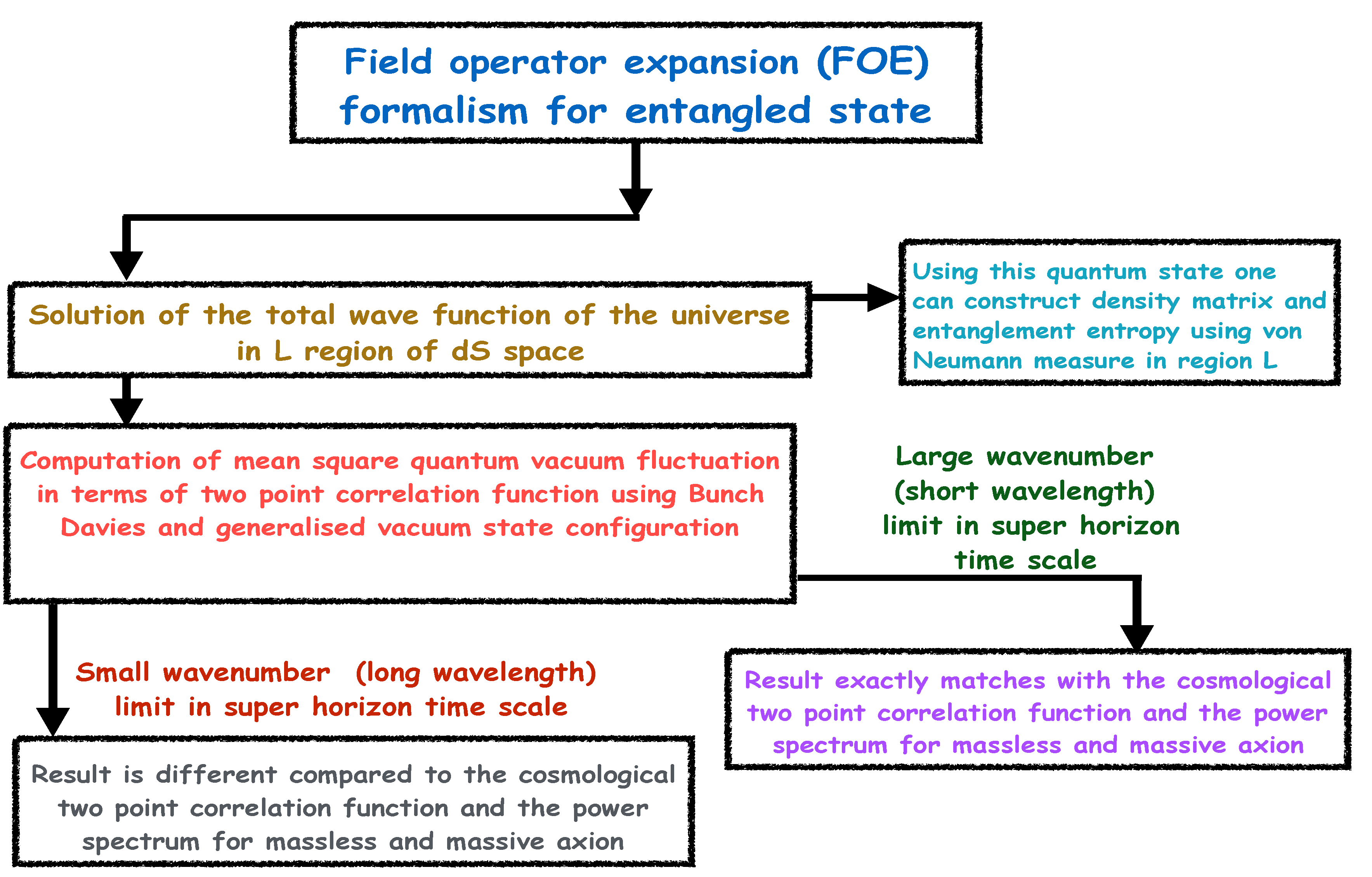
• Field operator expansion (FOE) method:
  This method is useful for entangled quantum states with the wave function of the de Sitter universe for Bunch Davies and most generalised $\alpha$ vacua. Technically this formalism is based on the wave function ${\chi }^{\mathcal{I}}$ which we will explicitly derive. The cosmological spectrum is characterised by the two point correlation function and their associated power spectrum. Using such entangled state in this formalism one can construct the usual density matrix for Bunch Davies and most generalised $\alpha$ vacua.
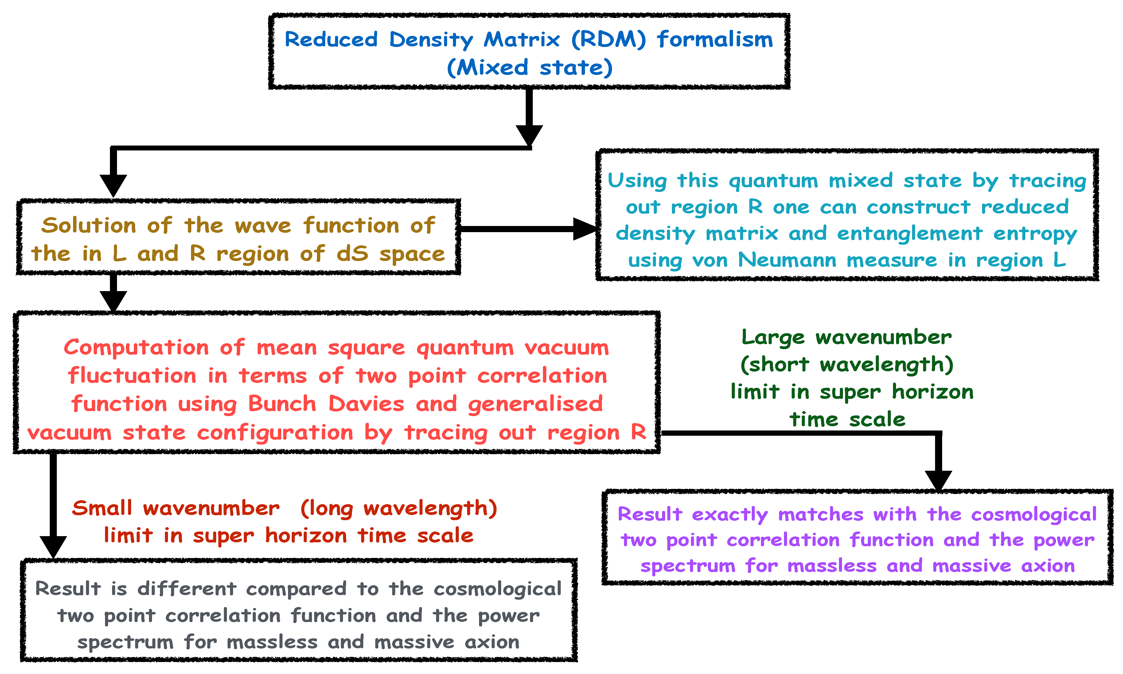
• Reduced density matrix (RDM) formalism:
  This formalism is helpful for mixed quantum states and is useful for the construction of reduced density matrix in a diagonalised representation of Bunch Davies and $\alpha$ vacua by tracing over the all possible degrees of freedom from the region R. Technically the formalism is based on the wave function ${\psi }^{\mathcal{I}}$ which we explicitly derive.
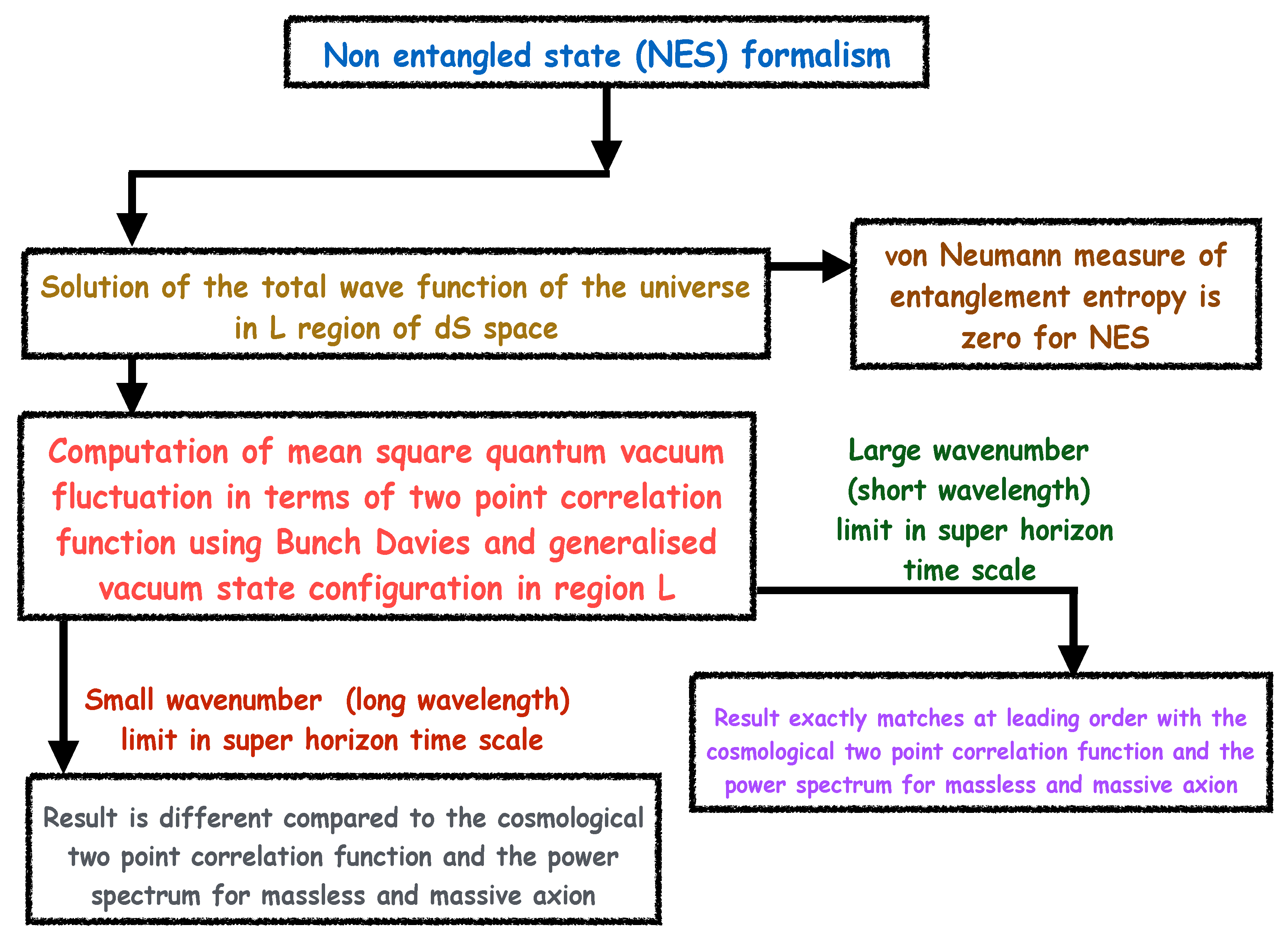
• Non entangled state (NES) formalism:
  This formalism in presence of non entangled quantum state which deals with the construction of wave function in the region L in which the total universe is described. Here we also use Bunch Davies and most generalised $\alpha$ vacua in the region L. Technically this formalism is based on the wave function ${\varphi }^{\mathcal{I}}$ which we explicitly derive in this paper.

We will now derive the expression for the mean square fluctuation considering both Bunch Davies vacuum and $\alpha$ vacua using the results presented in the previous section. For this computation we will follow the steps which are outlined below:

• First of all, we trace out all contributions which belong to the R region. As a result, the required field operator is only defined in the L region. This method we use in FOE formalism where the quantum states for L and R region are entangled with each other. On the other hand, doing a partial trace over region R one can construct reduced density matrix which leads to RDM formalism. Instead, if we use the non entangled quantum state and compute the wave function solely in L region we will be lead to the NES formalism. Please note that all of these three methods are used to compute mean square vacuum fluctuation or more precisely the quantum mechanical computation of two point correlation function for axion and the associated power spectrum.
• Instead of doing the computation in $|\mathbf{L}\rangle$ basis we use a new basis $|{\mathbf{L}}^{{}^{\prime }}\rangle$, obtained by applying Bogoliubov transformation in $|\mathbf{L}\rangle$. Consequently the field operators will act on $|{\mathbf{L}}^{{}^{\prime }}\rangle$ and the FOE method is developed in this transformed basis. On the other hand, as mentioned earlier it will appear in the expression for the reduced density matrix to be used in the RDM formalism. However, in the NES formalism this transformation is not very useful since in this case the total wave function is solely described by the quantum mechanical state appearing in the L region and the corresponding Hilbert space is spanned by only $|\mathbf{L}\rangle$ which forms a complete basis.
• Furthermore, we will compute the expressions for the mean square quantum vacuum fluctuation and the corresponding cosmological power spectrum after horizon exit using all the three formalisms, i.e., FOE, RDM, and NES. We will finally consider two limiting situations: long wave length and short wave length approximation for the computation of the power spectrum.

3.1. Quantum Vacuum Fluctuation Using Field Operator Expansion (FOE) (with Entangled State)

3.1.1. Wave Function in Field Operator Expansion (FOE)

Let us first compute the spectrum of vacuum fluctuation using field operator expansion (FOE). In Figure 5 we present a schematic diagram for the computation algorithm of field operator expansion method for entangled state of axion in de Sitter hyperbolic open chart. To compute the vacuum fluctuation using FOE, we focus only with the left region L as it is completely symmetric to the right region R. We use the time dependent mode function for the left region L which we presented in Section 2. Thus, instead of getting a $(4\times 4)$ square matrix (when both sectors are considered) we have a $(4\times 2)$ matrix which appears in the solution of the field equation as:

$$\begin{array}{c}\hfill \widetilde{{\chi }^I}=\frac{1}{{\mathcal{N}}_p}{\tilde{\mathcal{M}}}_{\mathcal{J}}^I{\tilde{\mathcal{P}}}^{\mathcal{J}}+\sum _{n=0}^{\infty }\frac{1}{{\mathcal{N}}_{p,\left(n\right)}}\tilde{{\left({\mathcal{M}}_{\left(n\right)}\right)}_{\mathcal{J}}^I}{\tilde{\mathcal{P}}}_{\left(n\right)}^{\mathcal{J}},\end{array}$$

(24)

where the index $\mathcal{J}=1,2$ is appearing for the contribution from region L. To write down the total solution in region L we define the following matrices:

$$\begin{array}{ccc}\hfill {\tilde{\mathcal{M}}}_{\mathcal{J}}^I& =& \left(\begin{array}{cc}{\alpha }_{\mathbf{L}}^{\sigma }& {\beta }_{\mathbf{L}}^{\sigma }\\ {\beta }_{\mathbf{L}}^{{\sigma }^{*}}& {\alpha }_{\mathbf{L}}^{{\sigma }^{*}}\end{array}\right),\tilde{{\left({\mathcal{M}}_{\left(n\right)}\right)}_{\mathcal{J}}^I}=\left(\begin{array}{cc}{\overline{\alpha }}_{\mathbf{L},n}^{\sigma }& {\overline{\beta }}_{\mathbf{L},n}^{\sigma }\\ {\overline{\beta }}_{\mathbf{L},n}^{{\sigma }^{*}}& {\overline{\alpha }}_{\mathbf{L},n}^{{\sigma }^{*}}\end{array}\right),\hfill \end{array}$$

(25)

$$\begin{array}{ccc}\hfill \widetilde{{\chi }^I}& =& \left(\begin{array}{c}{\chi }^{\sigma }\left(t\right)\\ {\chi }^{\sigma *}\left(t\right),\end{array}\right),{\tilde{\mathcal{P}}}^{\mathcal{J}}=\left(\begin{array}{c}{\tilde{\mathcal{P}}}^{\mathbf{L}}\\ {\tilde{\mathcal{P}}}^{{\mathbf{L}}^{*}},\end{array}\right),{\tilde{\mathcal{P}}}_{\left(n\right)}^{\mathcal{J}}=\left(\begin{array}{c}{\tilde{\mathcal{P}}}^{\mathbf{L},n}\\ {\tilde{\mathcal{P}}}^{{\mathbf{L}}^{*},n}\end{array}\right),\hfill \end{array}$$

(26)

where $\sigma =\pm 1$, $I=1,2,3,4$ and $\mathcal{J}=1,2$. The Fourier mode of the field operator, which is also the total solution of the field equation for axion (in presence of source contribution) can be expressed as:

$$\begin{array}{c}\hfill \widetilde{\mathsf{\Phi }\left(t_{\mathbf{L}}\right)}=\frac{H}{sinh{t}_{\mathbf{L}}}{Q}_I\widetilde{{\chi }^I}=\frac{H}{sinh{t}_{\mathbf{L}}}{Q}_I\left[\frac{1}{{\mathcal{N}}_p}{\tilde{\mathcal{M}}}_{\mathcal{J}}^I{\tilde{\mathcal{P}}}^J+\sum _{n=0}^{\infty }\frac{1}{{\mathcal{N}}_{p,\left(n\right)}}\tilde{{\left({\mathcal{M}}_{\left(n\right)}\right)}_{\mathcal{J}}^I}{\tilde{\mathcal{P}}}_{\left(n\right)}^{\mathcal{J}}\right],\end{array}$$

(27)

where the operator $Q_I$ represent a set of creation and annihilation operators which are defined (in Section 2) for Bunch Davies vacuum ($\alpha =0$) and $\alpha$ vacua ($\alpha \ne 0$) as:

$$\begin{array}{c}\hfill {\displaystyle Q_I\equiv \left\{\begin{array}{cc}{\displaystyle a_I=(a_{\sigma },a_{\sigma }^{†})=\left[a_I^{\left(c\right)}+\sum _{n=0}^{\infty }{a}_{I\left(n\right)}^{\left(p\right)}\right]}\hfill & \mathbf{for}\mathbf{Bunch}\mathbf{Davies}\mathbf{vacuum}\hfill \\ {\displaystyle d_I=(d_{\sigma },d_{\sigma }^{†})=\left[d_I^{\left(c\right)}+\sum _{n=0}^{\infty }{d}_{I\left(n\right)}^{\left(p\right)}\right]}\hfill & \mathbf{for}\alpha \mathbf{vacua}.\hfill \end{array}\right.}\end{array}$$

(28)

Here we labeled the time coordinate t by $t_{\mathbf{L}}$ since we are considering the left region L only.

To explicitly write down the expression for the amplitude of the normalized power spectrum, we start with the column matrix representation of the time dependent part of the solution of the wave function, given by:

$$\begin{array}{ccc}\hfill \widetilde{{\chi }^I}& =& \left(\begin{array}{c}{\chi }^{\sigma }\left(t\right)\\ {\chi }^{\sigma *}\left(t\right)\end{array}\right)=\left(\begin{array}{c}{\mathcal{A}}_{\mathbf{L}}^{\sigma }{\tilde{\mathcal{P}}}^{\mathbf{L}}+{\mathcal{B}}_{\mathbf{L}}^{\sigma }{\tilde{\mathcal{P}}}^{\mathbf{L}*}\\ {\mathcal{B}}_{\mathbf{L}}^{\sigma *}{\tilde{\mathcal{P}}}^{\mathbf{L}}+{\mathcal{A}}_{\mathbf{L}}^{\sigma *}{\tilde{\mathcal{P}}}^{\mathbf{L}*}\end{array}\right)+\sum _{n=0}^{\infty }\left(\begin{array}{c}{\mathcal{A}}_{\mathbf{L},\left(n\right)}^{\sigma }{\tilde{\mathcal{P}}}_{\left(n\right)}^{\mathbf{L}}+{\mathcal{B}}_{\mathbf{L},\left(n\right)}^{\sigma }{\tilde{\mathcal{P}}}_{\left(n\right)}^{\mathbf{L}*}\\ {\mathcal{B}}_{\mathbf{L},\left(n\right)}^{\sigma *}{\tilde{\mathcal{P}}}_{\left(n\right)}^{\mathbf{L}}+{\mathcal{A}}_{\mathbf{L},\left(n\right)}^{\sigma *}{\tilde{\mathcal{P}}}_{\left(n\right)}^{\mathbf{L}*}\end{array}\right),\hfill \end{array}$$

(29)

where the entries of the column matrix for the complementary and particular integral part of the solution are given by the following expressions:

$$\begin{array}{ccc}\hfill {\mathcal{A}}_{\mathbf{L}}^{\sigma }& =& \frac{{\alpha }_{\mathbf{L}}^{\sigma }}{{\mathcal{N}}_p}=\sigma \frac{e^{\pi p}-i\sigma e^{-i\pi \nu }}{{\mathcal{N}}_p\Gamma \left(\nu +ip+\frac{1}{2}\right)},\hfill \end{array}$$

(30)

$$\begin{array}{ccc}\hfill {\mathcal{B}}_{\mathbf{L}}^{\sigma }& =& \frac{{\beta }_{\mathbf{L}}^{\sigma }}{{\mathcal{N}}_p}=-\sigma \frac{e^{-\pi p}-i\sigma e^{-i\pi \nu }}{{\mathcal{N}}_p\Gamma \left(\nu -ip+\frac{1}{2}\right)},\hfill \end{array}$$

(31)

$$\begin{array}{ccc}\hfill {\mathcal{A}}_{\mathbf{L},\left(n\right)}^{\sigma }& =& \frac{{\alpha }_{\mathbf{L},\left(\mathbf{n}\right)}^{\sigma }}{{\mathcal{N}}_{p,\left(n\right)}}=\sigma \frac{e^{\pi p_n}-i\sigma e^{-i\pi \nu }}{{\mathcal{N}}_{p,\left(n\right)}\Gamma \left(\nu +i{p}_n+\frac{1}{2}\right)},\hfill \end{array}$$

(32)

$$\begin{array}{ccc}\hfill {\mathcal{B}}_{\mathbf{L},\left(n\right)}^{\sigma }& =& \frac{{\beta }_{\mathbf{L},\left(n\right)}^{\sigma }}{{\mathcal{N}}_{p,\left(n\right)}}=-\sigma \frac{e^{-\pi p_n}-i\sigma e^{-i\pi \nu }}{{\mathcal{N}}_{p,\left(n\right)}\Gamma \left(\nu -i{p}_n+\frac{1}{2}\right)}.\hfill \end{array}$$

(33)

${\mathcal{N}}_p$ and ${\mathcal{N}}_{p,\left(n\right)}$ in the above equations are the normalization constants for the complementary part and particular integral part of the solution as defined Section 2.

3.1.2. Two Point Correlation Function

To compute the expression for the two point correlation function for the vacuum fluctuation let us now concentrate on a single mode with fixed value of the $\mathbf{SO}(\mathbf{3},\mathbf{1})$ quantum numbers p, l and m. As a result, the mean square vacuum fluctuation of axion for any generalized arbitrary vacuum state ($|\mathsf{\Omega }\rangle$) can be expressed as:

$$\begin{array}{ccc}\hfill \langle \mathsf{\Omega }\left|\widetilde{{\mathsf{\Phi }}_{plm}\left(t_{\mathbf{L}}\right)}{\left(\tilde{{\mathsf{\Phi }}_{p^{{}^{\prime }}{l}^{{}^{\prime }}{m}^{{}^{\prime }}}\left(t_{\mathbf{L}}\right)}\right)}^{†}\right|\mathsf{\Omega }\rangle & =& \frac{H^2}{{sinh}^2{t}_{\mathbf{L}}}\langle \mathsf{\Omega }|{\left[Q_I\widetilde{{\chi }^I}\right]}_{plm}{\left({\left[Q_I\widetilde{{\chi }^I}\right]}_{p^{{}^{\prime }}{l}^{{}^{\prime }}{m}^{{}^{\prime }}}\right)}^{†}|\mathsf{\Omega }\rangle .\hfill \end{array}$$

(34)

Furthermore, explicitly writing the expression for the mean square vacuum fluctuation of axion for Bunch Davies vacuum we get the following simplified expressions:

$$\begin{array}{ccc}\langle \mathbf{BD}\left|\widetilde{{\mathsf{\Phi }}_{plm}\left(t_{\mathbf{L}}\right)}{\left(\tilde{{\mathsf{\Phi }}_{p^{{}^{\prime }}{l}^{{}^{\prime }}{m}^{{}^{\prime }}}\left(t_{\mathbf{L}}\right)}\right)}^{†}\right|\mathbf{BD}\rangle \hfill & =\hfill & \frac{H^2}{{sinh}^2{t}_{\mathbf{L}}}\langle \mathbf{BD}|{\left[a_I\widetilde{{\chi }^I}\right]}_{plm}{\left({\left[a_I\widetilde{{\chi }^I}\right]}_{p^{{}^{\prime }}{l}^{{}^{\prime }}{m}^{{}^{\prime }}}\right)}^{†}|\mathbf{BD}\rangle \hfill \\ \hfill & =\hfill & \frac{H^2}{{sinh}^2{t}_{\mathbf{L}}}{\sum }_{\sigma =\pm 1}{\left|\widetilde{{\chi }^{\sigma }}\right|}^2\delta (p-p^{{}^{\prime }}){\delta }_{l{l}^{{}^{\prime }}}{\delta }_{m{m}^{{}^{\prime }}}\hfill \\ \hfill & \equiv \hfill & P_{\mathbf{BD}}(p,t_{\mathbf{L}})\delta (p-p^{{}^{\prime }}){\delta }_{l{l}^{{}^{\prime }}}{\delta }_{m{m}^{{}^{\prime }}},\hfill \end{array}$$

(35)

where we define the amplitude of the normalized power spectrum of axion as:

$$\begin{array}{c}\hfill {\mathcal{P}}_{\mathbf{BD}}(p,t_{\mathbf{L}})=\frac{p^3}{2{\pi }^2}{P}_{\mathbf{BD}}(p,t_{\mathbf{L}})=\frac{p^3}{2{\pi }^2}\frac{H^2}{{sinh}^2{t}_{\mathbf{L}}}\sum _{\sigma =\pm 1}{\left|\widetilde{{\chi }^{\sigma }}\right|}^2.\end{array}$$

(36)

Furthermore, using Equation (29) we compute the following expression, which is appearing in the expression for the amplitude of the normalized power spectrum:

$$\begin{array}{ccc}{\sum }_{\sigma =\pm 1}{\left|\widetilde{{\chi }^{\sigma }}\right|}^2={\sum }_{\sigma =\pm 1}{\left(\widetilde{{\chi }^{\sigma }}\right)}^{†}\widetilde{{\chi }^{\sigma }}\hfill & =\hfill & \left[\left({\left|{\mathcal{A}}_{\mathbf{L}}^{\sigma }\right|}^2+{\left|{\mathcal{B}}_{\mathbf{L}}^{\sigma }\right|}^2\right){\tilde{\mathcal{P}}}^{\mathbf{L}}{\tilde{\mathcal{P}}}^{\mathbf{L}*}+{\mathcal{A}}_{\mathbf{L}}^{\sigma }{\mathcal{B}}_{\mathbf{L}}^{\sigma *}{\left({\tilde{\mathcal{P}}}^{\mathbf{L}}\right)}^2+{\mathcal{A}}_{\mathbf{L}}^{\sigma *}{\mathcal{B}}_{\mathbf{L}}^{\sigma }{\left({\tilde{\mathcal{P}}}^{\mathbf{L}*}\right)}^2\right.\hfill \\ \hfill & \hfill & +{\sum }_{n=0}^{\infty }\left\{\left({\mathcal{A}}_{\mathbf{L}}^{\sigma }{\mathcal{A}}_{\mathbf{L},\left(n\right)}^{\sigma *}+{\mathcal{B}}_{\mathbf{L}}^{\sigma }{\mathcal{B}}_{\mathbf{L},\left(n\right)}^{\sigma *}\right){\tilde{\mathcal{P}}}^{\mathbf{L}}{\tilde{\mathcal{P}}}_{\left(n\right)}^{\mathbf{L}*}\right.\hfill \\ \hfill & \hfill & +\left({\mathcal{A}}_{\mathbf{L}}^{\sigma }{\mathcal{B}}_{\mathbf{L},\left(n\right)}^{\sigma *}+{\mathcal{A}}_{\mathbf{L},\left(n\right)}^{\sigma }{\mathcal{B}}_{\mathbf{L}}^{\sigma *}\right){\tilde{\mathcal{P}}}^{\mathbf{L}}{\tilde{\mathcal{P}}}_{\left(n\right)}^{\mathbf{L}}\hfill \\ \hfill & \hfill & \left.+\left({\mathcal{A}}_{\mathbf{L},\left(n\right)}^{\sigma *}{\mathcal{B}}_{\mathbf{L}}^{\sigma }+{\mathcal{A}}_{\mathbf{L}}^{\sigma *}{\mathcal{B}}_{\mathbf{L},\left(n\right)}^{\sigma }\right){\tilde{\mathcal{P}}}_{\left(n\right)}^{\mathbf{L}*}{\tilde{\mathcal{P}}}^{\mathbf{L}*}\right\}\hfill \\ \hfill & \hfill & +{\sum }_{n=0}^{\infty }{\sum }_{m=0}^{\infty }\left\{\left({\mathcal{A}}_{\mathbf{L},\left(n\right)}^{\sigma }{\mathcal{A}}_{\mathbf{L},\left(m\right)}^{\sigma *}+{\mathcal{B}}_{\mathbf{L},\left(n\right)}^{\sigma }{\mathcal{B}}_{\mathbf{L},\left(m\right)}^{\sigma *}\right){\tilde{\mathcal{P}}}_{\left(n\right)}^{\mathbf{L}}{\tilde{\mathcal{P}}}_{\left(m\right)}^{\mathbf{L}*}\right.\hfill \\ \hfill & \hfill & \left.\left.+{\mathcal{A}}_{\mathbf{L},\left(n\right)}^{\sigma }{\mathcal{B}}_{\mathbf{L},\left(m\right)}^{\sigma *}{\tilde{\mathcal{P}}}_{\left(n\right)}^{\mathbf{L}}{\tilde{\mathcal{P}}}_{\left(m\right)}^{\mathbf{L}}+{\mathcal{A}}_{\mathbf{L},\left(n\right)}^{\sigma *}{\mathcal{B}}_{\mathbf{L},\left(m\right)}^{\sigma }{\tilde{\mathcal{P}}}_{\left(n\right)}^{\mathbf{L}*}{\tilde{\mathcal{P}}}_{\left(m\right)}^{\mathbf{L}*}\right\}\right].\hfill \end{array}$$

(37)

Using Equation (37), the amplitude of the normalized power spectrum of axion from Bunch Davies vacuum can be expressed in all time scales of region L as

$$\begin{array}{ccc}{\mathcal{P}}_{\mathbf{BD}}(p,t_{\mathbf{L}})\hfill & =\hfill & \frac{p^3}{2{\pi }^2}\frac{H^2}{{sinh}^2{t}_{\mathbf{L}}}{\sum }_{\sigma =\pm 1}{\left|\widetilde{{\chi }^{\sigma }}\right|}^2\hfill \\ \hfill & =\hfill & \frac{p^3}{2{\pi }^2}\frac{H^2}{{sinh}^2{t}_{\mathbf{L}}}\left[\left({\left|{\mathcal{A}}_{\mathbf{L}}^{\sigma }\right|}^2+{\left|{\mathcal{B}}_{\mathbf{L}}^{\sigma }\right|}^2\right){\tilde{\mathcal{P}}}^{\mathbf{L}}{\tilde{\mathcal{P}}}^{\mathbf{L}*}+{\mathcal{A}}_{\mathbf{L}}^{\sigma }{\mathcal{B}}_{\mathbf{L}}^{\sigma *}{\left({\tilde{\mathcal{P}}}^{\mathbf{L}}\right)}^2+{\mathcal{A}}_{\mathbf{L}}^{\sigma *}{\mathcal{B}}_{\mathbf{L}}^{\sigma }{\left({\tilde{\mathcal{P}}}^{\mathbf{L}*}\right)}^2\right.\hfill \\ \hfill & \hfill & +{\sum }_{n=0}^{\infty }\left\{\left({\mathcal{A}}_{\mathbf{L}}^{\sigma }{\mathcal{A}}_{\mathbf{L},\left(n\right)}^{\sigma *}+{\mathcal{B}}_{\mathbf{L}}^{\sigma }{\mathcal{B}}_{\mathbf{L},\left(n\right)}^{\sigma *}\right){\tilde{\mathcal{P}}}^{\mathbf{L}}{\tilde{\mathcal{P}}}_{\left(n\right)}^{\mathbf{L}*}\right.\hfill \\ \hfill & \hfill & +\left({\mathcal{A}}_{\mathbf{L}}^{\sigma }{\mathcal{B}}_{\mathbf{L},\left(n\right)}^{\sigma *}+{\mathcal{A}}_{\mathbf{L},\left(n\right)}^{\sigma }{\mathcal{B}}_{\mathbf{L}}^{\sigma *}\right){\tilde{\mathcal{P}}}^{\mathbf{L}}{\tilde{\mathcal{P}}}_{\left(n\right)}^{\mathbf{L}}\hfill \\ \hfill & \hfill & \left.+\left({\mathcal{A}}_{\mathbf{L},\left(n\right)}^{\sigma *}{\mathcal{B}}_{\mathbf{L}}^{\sigma }+{\mathcal{A}}_{\mathbf{L}}^{\sigma *}{\mathcal{B}}_{\mathbf{L},\left(n\right)}^{\sigma }\right){\tilde{\mathcal{P}}}_{\left(n\right)}^{\mathbf{L}*}{\tilde{\mathcal{P}}}^{\mathbf{L}*}\right\}\hfill \\ \hfill & \hfill & +{\sum }_{n=0}^{\infty }{\sum }_{m=0}^{\infty }\left\{\left({\mathcal{A}}_{\mathbf{L},\left(n\right)}^{\sigma }{\mathcal{A}}_{\mathbf{L},\left(m\right)}^{\sigma *}+{\mathcal{B}}_{\mathbf{L},\left(n\right)}^{\sigma }{\mathcal{B}}_{\mathbf{L},\left(m\right)}^{\sigma *}\right){\tilde{\mathcal{P}}}_{\left(n\right)}^{\mathbf{L}}{\tilde{\mathcal{P}}}_{\left(m\right)}^{\mathbf{L}*}\right.\hfill \\ \hfill & \hfill & \left.\left.+{\mathcal{A}}_{\mathbf{L},\left(n\right)}^{\sigma }{\mathcal{B}}_{\mathbf{L},\left(m\right)}^{\sigma *}{\tilde{\mathcal{P}}}_{\left(n\right)}^{\mathbf{L}}{\tilde{\mathcal{P}}}_{\left(m\right)}^{\mathbf{L}}+{\mathcal{A}}_{\mathbf{L},\left(n\right)}^{\sigma *}{\mathcal{B}}_{\mathbf{L},\left(m\right)}^{\sigma }{\tilde{\mathcal{P}}}_{\left(n\right)}^{\mathbf{L}*}{\tilde{\mathcal{P}}}_{\left(m\right)}^{\mathbf{L}*}\right\}\right].\hfill \end{array}$$

(38)

However, it is not easy to extract any information from Equation (38) for cosmological predictions. Hence, we consider the superhorizon time scales ($t_{\mathbf{L}}>>1$) of region L. In such a case, the Legendre functions, appearing in the complementary part and the particular integral part of the time dependent solution, can be approximated as:

$$\begin{array}{ccc}\hfill \left({\tilde{\mathcal{P}}}^{\mathbf{L}},{\tilde{\mathcal{P}}}^{\mathbf{L}*}\right)& \equiv & P_{\nu -\frac{1}{2}}^{\pm ip}\left(cosh{t}_{\mathbf{L}}\right)\underrightarrow{t_{\mathbf{L}}>>1}\frac{2^{\nu -\frac{1}{2}}{\left(cosh{t}_{\mathbf{L}}\right)}^{\nu -\frac{1}{2}}\Gamma \left(\nu \right)}{\sqrt{\pi }\Gamma \left(\nu \mp ip+\frac{1}{2}\right)},\hfill \end{array}$$

(39)

$$\begin{array}{ccc}\hfill \left({\tilde{\mathcal{P}}}_{\left(n\right)}^{\mathbf{L}},{\tilde{\mathcal{P}}}_{\left(n\right)}^{\mathbf{L}*}\right)& \equiv & P_{\nu -\frac{1}{2}}^{\pm i{p}_n}\left(cosh{t}_{\mathbf{L}}\right)\underrightarrow{t_{\mathbf{L}}>>1}\frac{2^{\nu -\frac{1}{2}}{\left(cosh{t}_{\mathbf{L}}\right)}^{\nu -\frac{1}{2}}\Gamma \left(\nu \right)}{\sqrt{\pi }\Gamma \left(\nu \mp i{p}_n+\frac{1}{2}\right)}.\hfill \end{array}$$

(40)

Consequently, in the superhorizon time scales ($t_{\mathbf{L}}>>1$) of region L Equation (37) can be further simplified as:

$$\begin{array}{ccc}\hfill \sum _{\sigma =\pm 1}{\left|\widetilde{{\chi }^{\sigma }}\right|}^2=\sum _{\sigma =\pm 1}{\left(\widetilde{{\chi }^{\sigma }}\right)}^{†}\widetilde{{\chi }^{\sigma }}& \underrightarrow{t_{\mathbf{L}}>>1}& \widetilde{\mathcal{M}(p,\nu )}{\left(cosh{t}_{\mathbf{L}}\right)}^{2\nu -1}\hfill \end{array}$$

(41)

where the time independent function $\widetilde{\mathcal{M}(p,\nu )}$ is defined as:

$$\begin{array}{ccc}\widetilde{\mathcal{M}(p,\nu )}& =& \frac{2^{2\nu -1}{\left(\Gamma \left(\nu \right)\right)}^2}{\pi }\times {\displaystyle \sum _{\sigma =\pm 1}}\left[\frac{\left({\left|{\mathcal{A}}_{\mathbf{L}}^{\sigma }\right|}^2+{\left|{\mathcal{B}}_{\mathbf{L}}^{\sigma }\right|}^2\right)}{{\left|\Gamma \left(\nu +ip+\frac{1}{2}\right)\right|}^2}+\frac{{\mathcal{A}}_{\mathbf{L}}^{\sigma }{\mathcal{B}}_{\mathbf{L}}^{\sigma *}}{{\left(\Gamma \left(\nu -ip+\frac{1}{2}\right)\right)}^2}+\frac{{\mathcal{A}}_{\mathbf{L}}^{\sigma *}{\mathcal{B}}_{\mathbf{L}}^{\sigma }}{{\left(\Gamma \left(\nu +ip+\frac{1}{2}\right)\right)}^2}\right.\\ & & +{\displaystyle \sum _{n=0}^{\infty }}\left\{\frac{\left({\mathcal{A}}_{\mathbf{L}}^{\sigma }{\mathcal{A}}_{\mathbf{L},\left(n\right)}^{\sigma *}+{\mathcal{B}}_{\mathbf{L}}^{\sigma }{\mathcal{B}}_{\mathbf{L},\left(n\right)}^{\sigma *}\right)}{\Gamma \left(\nu -ip+\frac{1}{2}\right)\Gamma \left(\nu +i{p}_n+\frac{1}{2}\right)}+\frac{\left({\mathcal{A}}_{\mathbf{L}}^{\sigma }{\mathcal{B}}_{\mathbf{L},\left(n\right)}^{\sigma *}+{\mathcal{A}}_{\mathbf{L},\left(n\right)}^{\sigma }{\mathcal{B}}_{\mathbf{L}}^{\sigma *}\right)}{\Gamma \left(\nu -ip+\frac{1}{2}\right)\Gamma \left(\nu -i{p}_n+\frac{1}{2}\right)}\right.\\ & & \left.+\frac{\left({\mathcal{A}}_{\mathbf{L},\left(n\right)}^{\sigma *}{\mathcal{B}}_{\mathbf{L}}^{\sigma }+{\mathcal{A}}_{\mathbf{L}}^{\sigma *}{\mathcal{B}}_{\mathbf{L},\left(n\right)}^{\sigma }\right)}{\Gamma \left(\nu +i{p}_n+\frac{1}{2}\right)\Gamma \left(\nu +ip+\frac{1}{2}\right)}\right\}\\ & & +{\displaystyle \sum _{n=0}^{\infty }}{\displaystyle \sum _{m=0}^{\infty }}\left\{\frac{\left({\mathcal{A}}_{\mathbf{L},\left(n\right)}^{\sigma }{\mathcal{A}}_{\mathbf{L},\left(m\right)}^{\sigma *}+{\mathcal{B}}_{\mathbf{L},\left(n\right)}^{\sigma }{\mathcal{B}}_{\mathbf{L},\left(m\right)}^{\sigma *}\right)}{\Gamma \left(\nu -i{p}_n+\frac{1}{2}\right)\Gamma \left(\nu +i{p}_m+\frac{1}{2}\right)}\right.\\ & & \left.\left.+\frac{{\mathcal{A}}_{\mathbf{L},\left(n\right)}^{\sigma }{\mathcal{B}}_{\mathbf{L},\left(m\right)}^{\sigma *}}{\Gamma \left(\nu -i{p}_n+\frac{1}{2}\right)\Gamma \left(\nu -i{p}_m+\frac{1}{2}\right)}+\frac{{\mathcal{A}}_{\mathbf{L},\left(n\right)}^{\sigma *}{\mathcal{B}}_{\mathbf{L},\left(m\right)}^{\sigma }}{\Gamma \left(\nu +i{p}_n+\frac{1}{2}\right)\Gamma \left(\nu +i{p}_m+\frac{1}{2}\right)}\right\}\right].\end{array}$$

(42)

As a result, in the superhorizon time scales ($t_{\mathbf{L}}>>1$) of region L the amplitude of the normalized power spectrum of axion from Bunch Davies vacuum can be expressed as:

$$\begin{array}{ccc}\hfill {\mathcal{P}}_{\mathbf{BD}}(p,t_{\mathbf{L}})& =& \frac{p^3}{2{\pi }^2}\frac{H^2}{{sinh}^2{t}_{\mathbf{L}}}\sum _{\sigma =\pm 1}{\left|\widetilde{{\chi }^{\sigma }}\right|}^2\underrightarrow{t_{\mathbf{L}}>>1}\frac{p^3}{2{\pi }^2}{\left(cosh{t}_{\mathbf{L}}\right)}^{2\nu -3}{H}^2\widetilde{\mathcal{M}(p,\nu )}.\hfill \end{array}$$

(43)

Here, it is important to note that in the superhorizon time scales ($t_{\mathbf{L}}>>1$) of region L if we consider the massless case where we fix the mass parameter to be $\nu =3/2$, then the time dependent contribution can be approximated as:

$$\begin{array}{c}\hfill {\left(\frac{{\left(cosh{t}_{\mathbf{L}}\right)}^{2\nu -1}}{{sinh}^2{t}_{\mathbf{L}}}\right)}_{\nu =3/2}\underrightarrow{t_{\mathbf{L}}>>1}1.\end{array}$$

(44)

Consequently, in the superhorizon time scales of region L and for the massless axion case, the amplitude of the normalized power spectrum of axion from Bunch Davies vacuum can be expressed as:

$$\begin{array}{ccc}\hfill {\mathcal{P}}_{\mathbf{BD}}(p,t_{\mathbf{L}})& =& \frac{p^3}{2{\pi }^2}\frac{H^2}{{sinh}^2{t}_{\mathbf{L}}}\sum _{\sigma =\pm 1}{\left|\widetilde{{\chi }^{\sigma }}\right|}^2\underrightarrow{t_{\mathbf{L}}>>1,\nu =3/2}\frac{p^3}{2{\pi }^2}{H}^2\widetilde{\mathcal{M}(p,\nu =3/2)}.\hfill \end{array}$$

(45)

This implies that in the massless case, the amplitude of the vacuum fluctuation gets frozen with respect to the time scale when the associated modes exit the horizon.

Furthermore, to infer the exact wave number dependence of the amplitude of the normalized power spectrum from Bunch Davies vacuum we need to know the behaviour of the power spectrum at very short wavelengths ($p,p_n>>1$). In this limit it is expected that the power spectrum should match the result obtained for spatially flat universe. Please note that in the short wave length approximation the time independent function $\widetilde{\mathcal{M}(p>>1,\nu )}$ for any arbitrary mass parameter $\nu$ can be expressed as:

$$\begin{array}{ccc}\hfill \widetilde{\mathcal{M}(p>>1,\nu )}& =& \frac{2^{2(\nu -1)}{\left(\Gamma \left(\nu \right)\right)}^2}{p^3\pi }\widetilde{\mathcal{G}(p>>1)},\hfill \end{array}$$

(46)

where we defined a new function $\widetilde{\mathcal{G}(p>>1)}$ in the short wave length limit as:

$$\begin{array}{ccc}\widetilde{\mathcal{G}\left(p\right)}\hfill & =\hfill & \frac{1}{\left(1+\frac{1}{82944p^4}\right)}\times \hfill \\ \hfill & \hfill & \left[{\left(1+e^{-2\pi p}\right)}^2+{\sum }_{n=0}^{\infty }{\left(\frac{p}{p_n}\right)}^{\frac{3}{2}}\frac{\sqrt{1+\frac{1}{82944p^4}}}{\sqrt{1+\frac{1}{82944p_n^4}}}\left(1+2\left(e^{-2\pi p}+e^{-2\pi p_n}\right)+e^{-2\pi (p+p_n)}\right)\right.\hfill \\ \hfill & \hfill & \left.+{\sum }_{n=0}^{\infty }{\sum }_{m=0}^{\infty }\frac{p^3}{{\left(p_n{p}_m\right)}^{3/2}}\frac{\left(1+\frac{1}{82944p^4}\right)}{\sqrt{1+\frac{1}{82944p_n^4}}\sqrt{1+\frac{1}{82944p_m^4}}}{\left(1+e^{-\pi (p_m+p_n)}\right)}^2\right].\hfill \end{array}$$

(47)

The above equation implies that for very large $p,p_n>>1$ one can rewrite this as, $\widetilde{\mathcal{G}\left(p\right)}\sim 1+\cdots$, and all the ⋯ terms can be considered to be small correction terms. Also for the mass less case ($\nu =3/2$) and in the short wave length approximation, the time independent function $\widetilde{\mathcal{M}(p,\nu =3/2)}$ can be further simplified as:

$$\begin{array}{ccc}\hfill \widetilde{\mathcal{M}(p>>1,\nu =3/2)}& =& \frac{\widetilde{\mathcal{G}(p>>1)}}{2p^3}.\hfill \end{array}$$

(48)

Finally, in the superhorizon time scales ($t_{\mathbf{L}}>>1$) of region L, the amplitude of the normalized power spectrum of axion from Bunch Davies vacuum in the short wave length limit can be expressed as:

$$\begin{array}{ccc}{\mathcal{P}}_{\mathbf{BD}}(p>>1,t_{\mathbf{L}}>>1)\hfill & =\hfill & \frac{p^3}{2{\pi }^2}{\left(cosh{t}_{\mathbf{L}}\right)}^{2\nu -3}{H}^2\widetilde{\mathcal{M}(p,\nu )}\hfill \\ \hfill & =\hfill & {\left(2cosh{t}_{\mathbf{L}}\right)}^{2\nu -3}{\left(\frac{H}{2\pi }\right)}^2{\left(\frac{\Gamma \left(\nu \right)}{\Gamma \left(\frac{3}{2}\right)}\right)}^2\widetilde{\mathcal{G}(p>>1)}.\hfill \end{array}$$

(49)

Also for the massless case ($\nu =3/2$) in the superhorizon time scales ($t_{\mathbf{L}}>>1$) of region L the amplitude of the normalized power spectrum of axion from Bunch Davies vacuum in the short wave length limit can be simplified as:

$$\begin{array}{ccc}\hfill {\mathcal{P}}_{\mathbf{BD}}(p>>1,t_{\mathbf{L}}>>1)& =& \frac{p^3}{2{\pi }^2}{H}^2\widetilde{\mathcal{M}(p>>1,\nu =3/2)}={\left(\frac{H}{2\pi }\right)}^2\widetilde{\mathcal{G}(p>>1)}.\hfill \end{array}$$

(50)

Now, we generalize the above results for the two point correlation function and the associated power spectrum for $\alpha$ vacua. For $\alpha$ vacua the mean square vacuum fluctuation of axion in the short wave length limit can be expressed as:

$$\begin{array}{ccc}\langle \alpha \left|\widetilde{{\mathsf{\Phi }}_{plm}\left(t_{\mathbf{L}}\right)}{\left(\tilde{{\mathsf{\Phi }}_{p^{{}^{\prime }}{l}^{{}^{\prime }}{m}^{{}^{\prime }}}\left(t_{\mathbf{L}}\right)}\right)}^{†}\right|\alpha \rangle \hfill & =\hfill & \frac{H^2}{{sinh}^2{t}_{\mathbf{L}}}\langle \alpha |{\left[d_I\widetilde{{\chi }^I}\right]}_{plm}{\left({\left[d_I\widetilde{{\chi }^I}\right]}_{p^{{}^{\prime }}{l}^{{}^{\prime }}{m}^{{}^{\prime }}}\right)}^{†}|\alpha \rangle \hfill \\ \hfill & =\hfill & \frac{H^2}{{sinh}^2{t}_{\mathbf{L}}}{\sum }_{\sigma =\pm 1}{\left|\widetilde{{\chi }^{\sigma }}\right|}^2\delta (p-p^{{}^{\prime }}){\delta }_{l{l}^{{}^{\prime }}}{\delta }_{m{m}^{{}^{\prime }}}\hfill \\ \hfill & \equiv \hfill & P(p>>1,\alpha ,t_{\mathbf{L}})\delta (p-p^{{}^{\prime }}){\delta }_{l{l}^{{}^{\prime }}}{\delta }_{m{m}^{{}^{\prime }}}.\hfill \end{array}$$

(51)

where we defined the amplitude of the normalized power spectrum of axion in the short wave length limit as:

$$\begin{array}{ccc}\mathcal{P}(p>>1,\alpha ,t_{\mathbf{L}})\hfill & =\hfill & \frac{p^3}{2{\pi }^2}P(p>>1,\alpha ,t_{\mathbf{L}})\hfill \\ \hfill & =\hfill & P_{\mathbf{BD}}(p>>1,t_{\mathbf{L}})\left(cosh2\alpha -sinh2\alpha \right)\hfill \\ \hfill & =\hfill & exp(-2\alpha )P_{\mathbf{BD}}(p>>1,t_{\mathbf{L}}).\hfill \end{array}$$

(52)

In the above equation, $P_{\mathbf{BD}}(p,t_{\mathbf{L}})$ is defined as:

$$\begin{array}{ccc}\hfill P_{\mathbf{BD}}(p>>1,t_{\mathbf{L}})& =& \frac{p^3}{2{\pi }^2}\frac{H^2}{{sinh}^2{t}_{\mathbf{L}}}\sum _{\sigma =\pm 1}{\left|\widetilde{{\chi }^{\sigma }}\right|}^2.\hfill \end{array}$$

(53)

We carry out the same approximations as earlier and we note that in the superhorizon time scales ($t_{\mathbf{L}}>>1$) of region L the amplitude of the normalized power spectrum of axion in the short wave length limit from $\alpha$ vacua can be expressed as:

$$\mathcal{P}(p>>1,\alpha ,t_{\mathbf{L}}>>1)={\mathcal{P}}_{\mathbf{BD}}(p>>1,t_{\mathbf{L}}>>1)\left(cosh2\alpha -sinh2\alpha \right)=exp(-2\alpha ){\mathcal{P}}_{\mathbf{BD}}(p,t_{\mathbf{L}}>>1),$$

(54)

where the normalized power spectrum in superhorizon scale for Bunch Davies vacuum ${\mathcal{P}}_{\mathbf{BD}}(p>>1,t_{\mathbf{L}}>>1)$ is defined in Equation (59). Here it is important to note that with $\alpha =0$ then we can reproduce the results obtained for Bunch Davies vacuum.

In Figure 6a,b we show the behaviour of the power spectrum of the mean square vacuum fluctuation computed from FOE formalism in the short wave length regime for $\alpha =0$ and $\alpha =0.1$ and for fixed values of the mass parameter $\nu (=3/2,2,5/2,3,7/2)$ respectively. In both cases we found almost similar behaviour. Additionally, in Figure 6c we depicted the behaviour of the power spectrum with respect to the mass parameter $\nu$ with fixed values of the parameter $\alpha (=0,0.1,0.2,0.3,0.4)$. It is clear from this figure that the power spectrum shows two distinct behaviour in $1/2<\nu <1$ and $\nu >1$ region. For $1/2<\nu <1$ region, the amplitude of the normalized power spectrum decreases to a certain value but just after $\nu =1$ it increases.

On the other hand, to know the exact wavenumber dependence of the amplitude of the normalised power spectrum from Bunch Davies vacuum in the long wavelength limit we need to know the behaviour of the power spectrum at $p,p_n<<1$. In this limit it is expected that the power spectrum of axion match with the result obtained for spatially flat universe. Here the time independent function $\widetilde{\mathcal{M}(p<<1,\nu )}$ for any arbitrary mass parameter $\nu$ can be expressed as:

$$\begin{array}{ccc}\hfill \widetilde{\mathcal{M}(p<<1,\nu )}& =& \frac{2^{2(\nu -1)}{\left(\Gamma \left(\nu \right)\right)}^2}{\pi }\widetilde{\mathcal{G}(p<<1)},\hfill \end{array}$$

(55)

where we defined a new function $\widetilde{\mathcal{G}(p<<1)}$ in the long wave length limit as:

$$\widetilde{\mathcal{G}(p<<1)}=\frac{\pi }{{|\Gamma \left(\nu +\frac{1}{2}\right)|}^2}\left[1+\frac{{|\Gamma \left(\nu +\frac{1}{2}\right)|}^2}{{\left(\Gamma \left(\nu +\frac{1}{2}\right)\right)}^2}\left\{1+3e^{-\pi p}\sum _{n=0}^{\infty }{e}^{-\pi p_n}+2\sum _{n=0}^{\infty }\sum _{m=0}^{\infty }{e}^{-\pi (p_n+p_m)}\right\}\right].$$

(56)

This implies that for very small wave numbers $p,p_n<<1$, one can write, $\widetilde{\mathcal{G}(p<<1)}\sim \frac{\pi }{{|\Gamma \left(\nu +\frac{1}{2}\right)|}^2}\left[1+\cdots \right]$, where all the⋯ terms are small correction terms.

Also for the massless case ($\nu =3/2$) and in the long wave length approximation, the time independent function $\widetilde{\mathcal{M}(p<<1,\nu =3/2)}$ can further be simplified as:

$$\begin{array}{ccc}\hfill \widetilde{\mathcal{M}(p<<1,\nu =3/2)}& =& \frac{\widetilde{\mathcal{G}(p<<1)}}{2}.\hfill \end{array}$$

(57)

Finally, in the super horizon time scales ($t_{\mathbf{L}}>>1$) of region L the amplitude of the normalized power spectrum of axion from Bunch Davies vacuum, in the long wave length limit, can be expressed as:

$$\begin{array}{ccc}{\mathcal{P}}_{\mathbf{BD}}(p<<1,t_{\mathbf{L}}>>1)\hfill & =\hfill & \frac{p^3}{2{\pi }^2}{\left(cosh{t}_{\mathbf{L}}\right)}^{2\nu -3}{H}^2\widetilde{\mathcal{M}(p<<1,\nu )}\hfill \\ \hfill & =\hfill & {\left(2cosh{t}_{\mathbf{L}}\right)}^{2\nu -3}{\left(\frac{H}{2\pi }\right)}^2{p}^3{\left(\frac{\Gamma \left(\nu \right)}{\Gamma \left(\frac{3}{2}\right)}\right)}^2\widetilde{\mathcal{G}(p<<1)},\hfill \end{array}$$

(58)

and for the massless case ($\nu =3/2$) this simplifies to:

$$\begin{array}{ccc}\hfill {\mathcal{P}}_{\mathbf{BD}}(p<<1,t_{\mathbf{L}}>>1)& =& \frac{p^3}{2{\pi }^2}{H}^2\widetilde{\mathcal{M}(p<<1,\nu =3/2)}={\left(\frac{H}{2\pi }\right)}^2{p}^3\widetilde{\mathcal{G}(p<<1)}.\hfill \end{array}$$

(59)

Here it is important to note that both Equation (58) and Equation (59) are valid after horizon exit.

Next, we generalize the result for the two point correlation function and the associated power spectrum for $\alpha$ vacua. For $\alpha$ vacua the mean square vacuum fluctuation of axion in the long wave length limit can be expressed as:

$$\begin{array}{ccc}\langle \alpha \left|\widetilde{{\mathsf{\Phi }}_{plm}\left(t_{\mathbf{L}}\right)}{\left(\tilde{{\mathsf{\Phi }}_{p^{{}^{\prime }}{l}^{{}^{\prime }}{m}^{{}^{\prime }}}\left(t_{\mathbf{L}}\right)}\right)}^{†}\right|\alpha \rangle \hfill & =\hfill & \frac{H^2}{{sinh}^2{t}_{\mathbf{L}}}\langle \alpha |{\left[d_I\widetilde{{\chi }^I}\right]}_{plm}{\left({\left[d_I\widetilde{{\chi }^I}\right]}_{p^{{}^{\prime }}{l}^{{}^{\prime }}{m}^{{}^{\prime }}}\right)}^{†}|\alpha \rangle \hfill \\ \hfill & =\hfill & \frac{H^2}{{sinh}^2{t}_{\mathbf{L}}}{\sum }_{\sigma =\pm 1}{\left|\widetilde{{\chi }^{\sigma }}\right|}^2\delta (p-p^{{}^{\prime }}){\delta }_{l{l}^{{}^{\prime }}}{\delta }_{m{m}^{{}^{\prime }}}\hfill \\ \hfill & \equiv \hfill & P(p<<1,\alpha ,t_{\mathbf{L}})\delta (p-p^{{}^{\prime }}){\delta }_{l{l}^{{}^{\prime }}}{\delta }_{m{m}^{{}^{\prime }}},\hfill \end{array}$$

(60)

where the amplitude of the normalized power spectrum of axion at long wave length limit is defined as:

$$\begin{array}{ccc}\mathcal{P}(p<<1,\alpha ,t_{\mathbf{L}})\hfill & =\hfill & \frac{p^3}{2{\pi }^2}P(p<<1,\alpha ,t_{\mathbf{L}})\hfill \\ \hfill & =\hfill & P_{\mathbf{BD}}(p,t_{\mathbf{L}})\left(cosh2\alpha -sinh2\alpha \right)\hfill \\ \hfill & =\hfill & exp(-2\alpha )P_{\mathbf{BD}}(p<<1,t_{\mathbf{L}}),\hfill \end{array}$$

(61)

with $P_{\mathbf{BD}}(p<<1,t_{\mathbf{L}})$ as defined earlier.

In the super horizon time scales ($t_{\mathbf{L}}>>1$) of region L the amplitude of the normalized power spectrum of axion in the long wave length approximation from $\alpha$ vacua can be expressed as:

$$\begin{array}{ccc}\mathcal{P}(p<<1,\alpha ,t_{\mathbf{L}}>>1)\hfill & =\hfill & {\mathcal{P}}_{\mathbf{BD}}(p<<1,t_{\mathbf{L}}>>1)\left(cosh2\alpha -sinh2\alpha \right)\hfill \\ \hfill & =\hfill & exp(-2\alpha ){\mathcal{P}}_{\mathbf{BD}}(p<<1,t_{\mathbf{L}}>>1),\hfill \end{array}$$

(62)

where ${\mathcal{P}}_{\mathbf{BD}}(p<<1,t_{\mathbf{L}}>>1)$ is defined in Equation (58). It may be noted that for $\alpha =0$ we get back the results obtained for Bunch Davies vacuum.

In Figure 7a–c we show the behaviour of the power spectrum of the mean square vacuum fluctuation computed from FOE formalism in the small wave number regime. The values of $\alpha$ and the values of the mass parameter $\nu$ used here are same as those taken for large wave number regime. As expected, the behaviour for the the two limiting cases are distinct. However, the characteristics observed for $\alpha$ and $\nu$ dependences for both cases are almost similar.

3.2. Quantum Vacuum Fluctuation Using Reduced Density Matrix (RDM) Formalism (with Mixed State)

In this section, we study the features of the two point correlation function of the quantum vacuum fluctuations and the associated primordial power spectrum using the reduced density matrix formalism. In Figure 8 we present a schematic diagram for the computation algorithm of reduced density matrix formalism for mixed quantum state of axion in de Sitter hyperbolic open chart.

3.2.1. Reduced Density Matrix (RDM) Formalism

We first write down the Fourier mode of the field operator, which is also the total solution of the field equation for axion in presence of source contribution. We start directly from the solution obtained in Equation (20) and rewrite it in terms of the following matrix equation:

$$\begin{array}{c}\hfill {\mathsf{Ø}}^I=\frac{1}{{\mathcal{N}}_p}{\mathcal{M}}_J^I{\mathcal{P}}^J+\sum _{n=0}^{\infty }\frac{1}{{\mathcal{N}}_{p,\left(n\right)}}{\left({\mathcal{M}}_{\left(n\right)}\right)}_J^I{\mathcal{P}}_{\left(n\right)}^J\end{array}$$

(63)

where for the complementary part of the solution we defined the following matrices:

$$\begin{array}{ccc}\hfill {\mathcal{M}}_J^I& =& \left(\begin{array}{cc}{\alpha }_q^{\sigma }& {\beta }_q^{\sigma }\\ {\beta }_q^{{\sigma }^{*}}& {\alpha }_q^{{\sigma }^{*}}\end{array}\right),{\chi }^I=\left(\begin{array}{c}{\chi }_{\sigma }\left(t\right)\\ {\chi }_{\sigma }^{*}\left(t\right),\end{array}\right),{\mathcal{P}}^J=\left(\begin{array}{c}{\mathcal{P}}^q\\ {\mathcal{P}}^{q^{*}},\end{array}\right).\hfill \end{array}$$

(64)

Similarly for the particular solution, we define the following matrices:

$$\begin{array}{ccc}\hfill {\left({\mathcal{M}}_{\left(n\right)}\right)}_J^I& =& \left(\begin{array}{cc}{\overline{\alpha }}_{q,n}^{\sigma }& {\overline{\beta }}_{q,n}^{\sigma }\\ {\overline{\beta }}_{q,n}^{{\sigma }^{*}}& {\overline{\alpha }}_{q,n}^{{\sigma }^{*}}\end{array}\right),{\mathcal{P}}_{\left(n\right)}^J=\left(\begin{array}{c}{\mathcal{P}}^{q,n}\\ {\mathcal{P}}^{q^{*},n}\end{array}\right),\hfill \end{array}$$

(65)

where $\sigma =\pm 1$, $q=\mathbf{R},\mathbf{L}$ and $I,J=1,2,3,4$.

The redefined normalization constant for the particular part of the solution ${\mathcal{N}}_{p,\left(n\right)}$ can be expressed as, ${\mathcal{N}}_{p,\left(n\right)}=2sinh\pi p_n\sqrt{{\mathcal{N}}_{p_n\sigma }}\left(p^2-p_n^2\right)$. Furthermore, using Equation (63) the Bunch-Davies mode function can be written as:

$$\begin{array}{c}\hfill \frac{H}{sinht}{a}_I{\chi }^I=\frac{H}{sinht}{a}_I\left[\frac{1}{{\mathcal{N}}_p}{\mathcal{M}}_J^I{\mathcal{P}}^J+\sum _{n=0}^{\infty }\frac{1}{{\mathcal{N}}_{p,\left(n\right)}}{\left({\mathcal{M}}_{\left(n\right)}\right)}_J^I{\mathcal{P}}_{\left(n\right)}^J\right],\end{array}$$

(66)

where $a_I=(a_{\sigma },a_{\sigma }^{†})$ represents a set of creation and annihilation operators.

We also define the following operators:

$$\begin{array}{ccc}\hfill b_J& =& a_I^{\left(c\right)}{\mathcal{M}}_J^I,b_{J\left(n\right)}=a_{I\left(n\right)}^{\left(p\right)}{\left({\mathcal{M}}_{\left(n\right)}\right)}_J^I,\hfill \end{array}$$

(67)

where $a_I^{\left(c\right)}=(a_{\sigma }^{\left(c\right)},a_{\sigma }^{\left(c\right)†})$ and $a_{I\left(n\right)}^{\left(p\right)}=(a_{\sigma ,n}^{\left(p\right)},a_{\sigma ,n}^{\left(p\right)†})$ are the set of creation and annihilation operators which act on the complementary and particular part respectively. Thus, the operator contribution for the total solution is:

$$\begin{array}{ccc}\hfill a_I& =& \left[a_I^{\left(c\right)}+\sum _{n=0}^{\infty }{a}_{I\left(n\right)}^{\left(p\right)}\right],\hfill \end{array}$$

(68)

where by inverting Equation (67) we expressed:

$$\begin{array}{ccc}\hfill a_I^{\left(c\right)}& =& b_J{\left({\mathcal{M}}^{-1}\right)}_J^I,a_{I\left(n\right)}^{\left(p\right)}=b_{J\left(n\right)}{\left({\mathcal{M}}_{\left(n\right)}^{-1}\right)}_J^I.\hfill \end{array}$$

(69)

The inverse matrices are defined as:

$$\begin{array}{ccc}\hfill {\left({\mathcal{M}}^{-1}\right)}_J^I& =& \left(\begin{array}{cc}{\gamma }_{\sigma q}& {\delta }_{\sigma q}\\ {\delta }_{\sigma q}^{*}& {\gamma }_{\sigma q}^{*}\end{array}\right),{\left({\mathcal{M}}_{\left(n\right)}^{-1}\right)}_J^I=\left(\begin{array}{cc}{\overline{\gamma }}_{\sigma q,n}& {\overline{\delta }}_{\sigma q,n}\\ {\overline{\delta }}_{\sigma q,n}^{*}& {\overline{\gamma }}_{\sigma q,n}^{*}\end{array}\right),\hfill \end{array}$$

(70)

where $\sigma =\pm 1$, $q=\mathbf{R},\mathbf{L}$ and $I,J=1,2,3,4$.

For further computation, $\alpha$-vacua are defined in terms of Bunch Davies vacuum state as:

$$\begin{array}{ccc}\hfill |\alpha \rangle & =& exp\left({\displaystyle \frac{1}{2}tanh\alpha \sum _{\sigma =\pm 1}{a}_{\sigma }^{†}{a}_{\sigma }}\right)|\mathbf{BD}\rangle .\hfill \end{array}$$

(71)

It is to be noted that for $\alpha =0$ we get, $|\alpha =0\rangle =|0\rangle =|\mathbf{BD}\rangle .$ Moreover, we can also write the $\mathbf{R}$ and $\mathbf{L}$ vacua as:

$$\begin{array}{ccc}\hfill |\mathbf{R}\rangle & =& {|\mathbf{R}\rangle }_{\left(c\right)}+\sum _{n=0}^{\infty }{|\mathbf{R}\rangle }_{\left(p\right),n},|\mathbf{L}\rangle ={|\mathbf{L}\rangle }_{\left(c\right)}+\sum _{n=0}^{\infty }{|\mathbf{L}\rangle }_{\left(p\right),n},\hfill \end{array}$$

(72)

with subscripts $\left(c\right)$ and $\left(p\right)$ representing the complementary and particular part respectively.

Furthermore, assuming the bipartite Hilbert space (${\mathcal{H}}_{\alpha }:={\mathcal{H}}_{\mathbf{R}}\otimes {\mathcal{H}}_{\mathbf{L}}$) one can also write the $\alpha$-vacua in terms of the $\mathbf{R}$ and $\mathbf{L}$ vacuum as:

$$|\alpha \rangle =exp\left({\displaystyle \frac{1}{2}tanh\alpha \sum _{\sigma =\pm 1}{a}_{\sigma }^{†}{a}_{\sigma }}\right)\underset{\mathbf{Bunch}-\mathbf{Davies}\mathbf{contribution}}{\underbrace{exp\left(\frac{1}{2}\sum _{i,j=\mathbf{R},\mathbf{L}}{m}_{ij}{b}_i^{†}{b}_j^{†}+\frac{1}{2}\sum _{i,j=\mathbf{R},\mathbf{L}}\sum _{n=0}^{\infty }{\overline{m}}_{ij,n}{\overline{b}}_{i,n}^{†}{\overline{b}}_{j,n}^{†}\right)\left(\right|\mathbf{R}\rangle \otimes |\mathbf{L}\rangle )}},$$

(73)

where the matrices $m_{ij}$ and ${\overline{m}}_{ij,n}$ are defined for the complementary and particular part of the solution obtained for Bunch Davies vacuum state. In other words by setting $\alpha =0$ we get the following expression for the Bunch Davies quantum state:

$$|\mathbf{BD}\rangle =exp\left(\frac{1}{2}\sum _{i,j=\mathbf{R},\mathbf{L}}{m}_{ij}{b}_i^{†}{b}_j^{†}+\frac{1}{2}\sum _{i,j=\mathbf{R},\mathbf{L}}\sum _{n=0}^{\infty }{\overline{m}}_{ij,n}{\overline{b}}_{i,n}^{†}{\overline{b}}_{j,n}^{†}\right)\left(\right|\mathbf{R}\rangle \otimes |\mathbf{L}\rangle ).$$

(74)

Also the creation and annihilation operators for the $\mathbf{R}$ and $\mathbf{L}$ vacuum are defined in terms of new b type of oscillators using Bogoliubov transformation as:

$$\begin{array}{ccc}\hfill a_{\sigma }& =& \sum _{q=\mathbf{R},\mathbf{L}}\left\{\left[{\gamma }_{q\sigma }{b}_q+{\delta }_{q\sigma }^{*}{b}_q^{†}\right]+\sum _{n=0}^{\infty }\left[{\overline{\gamma }}_{q\sigma ,n}{\overline{b}}_{q,n}+{\overline{\delta }}_{q\sigma ,n}^{*}{\overline{b}}_{q,n}^{†}\right]\right\}\forall \sigma =\pm 1,\hfill \end{array}$$

(75)

$$\begin{array}{ccc}\hfill a_{\sigma }^{†}& =& \sum _{q=\mathbf{R},\mathbf{L}}\left\{\left[{\gamma }_{q\sigma }^{*}{b}_q^{†}+{\delta }_{q\sigma }{b}_q\right]+\sum _{n=0}^{\infty }\left[{\overline{\gamma }}_{q\sigma ,n}^{*}{\overline{b}}_{q,n}^{†}+{\overline{\delta }}_{q\sigma ,n}{\overline{b}}_{q,n}\right]\right\}\forall \sigma =\pm 1.\hfill \end{array}$$

(76)

Here ${\gamma }_{q\sigma }$, ${\delta }_{q\sigma }$, ${\overline{\gamma }}_{q\sigma ,n}$ and ${\overline{\delta }}_{q\sigma ,n}$ are the coefficient matrices. For our further computation we use the definition of $\alpha$-vacuum state (and Bunch Davies vacuum state), which is very useful to compute long range cosmological correlation functions in de Sitter space. In the context of $\alpha$-vacua the creation and annihilation operators are defined in terms of the constituents of $\mathbf{R}$ or $\mathbf{L}$ vacuum state as:

$$\begin{array}{ccc}{d}_{\sigma }\hfill & =\hfill & {\sum }_{q=\mathbf{R},\mathbf{L}}\left\{\left[\left(cosh\alpha {\gamma }_{q\sigma }-sinh\alpha {\delta }_{q\sigma }\right)b_q+\left(cosh\alpha {\delta }_{q\sigma }^{*}-sinh\alpha {\gamma }_{q\sigma }^{*}\right)b_q^{†}\right]\right.\hfill \\ \hfill & \hfill & +\left[\left(cosh\alpha {\sum }_{n=0}^{\infty }{\overline{\gamma }}_{q\sigma ,n}{\overline{b}}_{q,n}-sinh\alpha {\sum }_{n=0}^{\infty }{\overline{\delta }}_{q\sigma ,n}{\overline{b}}_{q,n}\right)\right.\hfill \\ \hfill & \hfill & \left.\left.+\left(cosh\alpha {\sum }_{n=0}^{\infty }{\overline{\delta }}_{q\sigma ,n}^{*}{\overline{b}}_{q,n}^{†}-sinh\alpha {\sum }_{n=0}^{\infty }{\overline{\gamma }}_{q\sigma ,n}^{*}{\overline{b}}_{q,n}^{†}\right)\right]\right\}\forall \sigma =\pm 1,\hfill \end{array}$$

(77)

$$\begin{array}{ccc}{d}_{\sigma }^{†}\hfill & =\hfill & {\sum }_{q=\mathbf{R},\mathbf{L}}\left\{\left[\left(cosh\alpha {\gamma }_{q\sigma }^{*}-sinh\alpha {\delta }_{q\sigma }^{*}\right)b_q^{†}+\left(cosh\alpha {\delta }_{q\sigma }-sinh\alpha {\gamma }_{q\sigma }\right)b_q\right]\right.\hfill \\ \hfill & \hfill & +\left[\left(cosh\alpha {\sum }_{n=0}^{\infty }{\overline{\gamma }}_{q\sigma ,n}^{*}{\overline{b}}_{q,n}^{†}-sinh\alpha {\sum }_{n=0}^{\infty }{\overline{\delta }}_{q\sigma ,n}^{*}{\overline{b}}_{q,n}^{†}\right)\right.\hfill \\ \hfill & \hfill & \left.\left.+\left(cosh\alpha {\sum }_{n=0}^{\infty }{\overline{\delta }}_{q\sigma ,n}{\overline{b}}_{q,n}-sinh\alpha {\sum }_{n=0}^{\infty }{\overline{\gamma }}_{q\sigma ,n}{\overline{b}}_{q,n}\right)\right]\right\}\forall \sigma =\pm 1,\hfill \end{array}$$

(78)

where we use the definition of creation and annihilation operators in Bunch Davies vacuum as mentioned in Equations (76) and (75). In this computation it is important to note that under Bogoliubov transformation the original matrix ${\gamma }_{q\sigma }$, ${\delta }_{q\sigma }$, ${\overline{\gamma }}_{q\sigma ,n}$ and ${\overline{\delta }}_{q\sigma ,n}$ used for Bunch Davies vacuum transform (for $\alpha$-vacua) as:

$$\begin{array}{ccc}\hfill {\gamma }_{q\sigma }& ⟶& \left(cosh\alpha {\gamma }_{q\sigma }-sinh\alpha {\delta }_{q\sigma }\right),{\delta }_{q\sigma }⟶\left(cosh\alpha {\delta }_{q\sigma }-sinh\alpha {\gamma }_{q\sigma }\right),\hfill \\ \hfill {\overline{\gamma }}_{q\sigma ,n}& ⟶& \left(cosh\alpha {\overline{\gamma }}_{q\sigma ,n}-sinh\alpha {\overline{\delta }}_{q\sigma ,n}\right),{\overline{\delta }}_{q\sigma ,n}⟶\left(cosh\alpha {\overline{\delta }}_{q\sigma ,n}-sinh\alpha {\overline{\gamma }}_{q\sigma ,n}\right).\hfill \end{array}$$

(79)

Thus, after the Bogoliubov transformation, $\alpha$-vacua state can be written in terms of $\mathbf{R}$ and $\mathbf{L}$ vacua as:

$$\begin{array}{ccc}\hfill |\alpha \rangle & =& exp\left(\frac{1}{2}\sum _{i,j=\mathbf{R},\mathbf{L}}{\tilde{m}}_{ij}{b}_i^{†}{b}_j^{†}+\frac{1}{2}\sum _{i,j=\mathbf{R},\mathbf{L}}\sum _{n=0}^{\infty }{\overline{\tilde{m}}}_{ij,n}{\overline{b}}_{i,n}^{†}{\overline{b}}_{j,n}^{†}\right)\left(\right|\mathbf{R}\rangle \otimes |\mathbf{L}\rangle ),\hfill \end{array}$$

(80)

Here ${\tilde{m}}_{ij}$ and ${\overline{\tilde{m}}}_{ij,n}$ represent the entries of the matrices corresponding to the complementary and particular solution respectively and we will compute them by demanding $d_{\sigma }|\alpha \rangle =0,$ and keeping only linear terms of creation operators. This directly yields the following:

$$\begin{array}{ccc}\hfill \left[{\tilde{m}}_{ij}\left(cosh\alpha {\gamma }_{j\sigma }-sinh\alpha {\delta }_{j\sigma }\right)+\left(cosh\alpha {\delta }_{i\sigma }^{*}-sinh\alpha {\gamma }_{i\sigma }^{*}\right)\right]& =& 0,\hfill \end{array}$$

(81)

$$\begin{array}{ccc}\hfill \left[\left(cosh\alpha {\overline{\tilde{m}}}_{ij,n}{\overline{\gamma }}_{j\sigma ,n}-sinh\alpha {\overline{m}}_{ij,n}{\overline{\delta }}_{j\sigma ,n}\right)+\left(cosh\alpha {\overline{\delta }}_{i\sigma ,n}^{*}-sinh\alpha {\overline{\gamma }}_{i\sigma ,n}^{*}\right)\right]& =& 0\forall n.\hfill \end{array}$$

(82)

From these two equations, the matrices corresponding to the complementary and particular part of the solution can be expressed as:

$$\begin{array}{ccc}\hfill {\tilde{m}}_{ij}& =& -\left(cosh\alpha {\delta }_{i\sigma }^{*}-sinh\alpha {\gamma }_{i\sigma }^{*}\right){\left(cosh\alpha \gamma -sinh\alpha \delta \right)}_{\sigma j}^{-1}=\left(\begin{array}{cc}{\tilde{m}}_{\mathbf{RR}}& {\tilde{m}}_{\mathbf{RL}}\\ {\tilde{m}}_{\mathbf{LR}}& {\tilde{m}}_{\mathbf{LL}}\end{array}\right),\hfill \end{array}$$

(83)

$$\begin{array}{ccc}\hfill {\overline{\tilde{m}}}_{ij,n}& =& -\left(cosh\alpha {\overline{\delta }}_{i\sigma ,n}^{*}-sinh\alpha {\overline{\gamma }}_{i\sigma ,n}^{*}\right){\left(cosh\alpha \overline{\gamma }-sinh\alpha \overline{\delta }\right)}_{\sigma j,n}^{-1}=\left(\begin{array}{cc}{\overline{m}}_{\mathbf{RR},n}& {\overline{m}}_{\mathbf{RL},n}\\ {\overline{m}}_{\mathbf{LR},n}& {\overline{m}}_{\mathbf{LL},n}\end{array}\right).\hfill \end{array}$$

(84)

Substituting the expressions for $\gamma$, $\delta$, ${\gamma }_n$ and ${\delta }_n$ we finally obtain the entries of the mass matrices for $i,j=\mathbf{R},\mathbf{L}$ as:

$$\begin{array}{c}\hfill {\tilde{m}}_{ij}=e^{i\theta }\frac{\sqrt{2}{e}^{-p\pi }{\mathcal{T}}_{ij}^{\left(\nu \right)}}{\sqrt{cosh2\pi p+cos2\pi \nu }\left({cosh}^2\alpha +{sinh}^2\alpha e^{-2\pi (p+i\nu )}\right)}\end{array}$$

(85)

$$\begin{array}{c}\hfill {\overline{\tilde{m}}}_{ij,n}=e^{i\theta }\frac{\sqrt{2}{e}^{-p_n\pi }{\mathcal{T}}_{ij}^{(\nu ,n)}}{\sqrt{cosh2\pi p_n+cos2\pi \nu }\left({cosh}^2\alpha +{sinh}^2\alpha e^{-2\pi (p_n+i\nu )}\right)}\end{array}$$

(86)

where we defined the $\mathcal{T}$ matrices as:

$$\begin{array}{ccc}\hfill {\mathcal{T}}_{ij}^{\left(\nu \right)}& =& \left(\begin{array}{cc}{\mathcal{T}}_{\mathbf{RR}}^{\left(\nu \right)}& {\mathcal{T}}_{\mathbf{RL}}^{\left(\nu \right)}\\ {\mathcal{T}}_{\mathbf{LR}}^{\left(\nu \right)}& {\mathcal{T}}_{\mathbf{LL}}^{\left(\nu \right)}\end{array}\right),{\mathcal{T}}_{ij}^{(\nu ,n)}=\left(\begin{array}{cc}{\mathcal{T}}_{\mathbf{RR}}^{(\nu ,n)}& {\mathcal{T}}_{\mathbf{RL}}^{(\nu ,n)}\\ {\mathcal{T}}_{\mathbf{LR}}^{(\nu ,n)}& {\mathcal{T}}_{\mathbf{LL}}^{(\nu ,n)}\end{array}\right).\hfill \end{array}$$

(87)

and the corresponding entries of the $\mathcal{T}$ matrices are given by:

$$\begin{array}{ccc}\hfill {\mathcal{T}}_{\mathbf{RR}}^{\left(\nu \right)}& =& {\mathcal{T}}_{\mathbf{LL}}^{\left(\nu \right)}=\left[\left({cosh}^2\alpha +{sinh}^2\alpha e^{-2i\pi \nu }\right)-sinh2\alpha {sinh}^2\pi p{e}^{-i\pi \nu }sec\pi \nu \right]cos\pi \nu ,\hfill \end{array}$$

(88)

$$\begin{array}{ccc}\hfill {\mathcal{T}}_{\mathbf{RL}}^{\left(\nu \right)}& =& {\mathcal{T}}_{\mathbf{LR}}^{\left(\nu \right)}=i\left[{cosh}^2\alpha +{sinh}^2\alpha e^{-2i\pi \nu }+sinh2\alpha cos\pi \nu e^{-i\pi \nu }\right]sinh\pi p,\hfill \end{array}$$

(89)

$$\begin{array}{ccc}\hfill {\mathcal{T}}_{\mathbf{RR}}^{(\nu ,n)}& =& {\mathcal{T}}_{\mathbf{LL}}^{(\nu ,n)}=\left[\left({cosh}^2\alpha +{sinh}^2\alpha e^{-2i\pi \nu }\right)-sinh2\alpha {sinh}^2\pi p_n{e}^{-i\pi \nu }sec\pi \nu \right]cos\pi \nu ,\hfill \end{array}$$

(90)

$$\begin{array}{ccc}\hfill {\mathcal{T}}_{\mathbf{RL}}^{(\nu ,n)}& =& {\mathcal{T}}_{\mathbf{LR}}^{(\nu ,n)}=i\left[{cosh}^2\alpha +{sinh}^2\alpha e^{-2i\pi \nu }+sinh2\alpha cos\pi \nu e^{-i\pi \nu }\right]sinh\pi p_n.\hfill \end{array}$$

(91)

For the massless ($\nu =3/2$) axion case, we obtain the following simplified expressions:

$$\begin{array}{c}\hfill {\tilde{m}}_{ij}=e^{i\theta }\frac{\sqrt{2}{e}^{-p\pi }{\mathcal{T}}_{ij}^{(3/2)}}{\sqrt{cosh2\pi p-1}\left({cosh}^2\alpha -{sinh}^2\alpha e^{-2\pi p}\right)}\end{array}$$

(92)

$$\begin{array}{c}\hfill {\overline{\tilde{m}}}_{ij,n}=e^{i\theta }\frac{\sqrt{2}{e}^{-p_n\pi }{\mathcal{T}}_{ij}^{(3/2,n)}}{\sqrt{cosh2\pi p_n-1}\left({cosh}^2\alpha -{sinh}^2\alpha e^{-2\pi p_n}\right)}\end{array}$$

(93)

where we defined the ${\mathcal{T}}^{(3/2)}$ matrices as:

$$\begin{array}{ccc}\hfill {\mathcal{T}}_{ij}^{(3/2)}& =& \left(\begin{array}{cc}{\mathcal{T}}_{\mathbf{RR}}^{(3/2)}& {\mathcal{T}}_{\mathbf{RL}}^{(3/2)}\\ {\mathcal{T}}_{\mathbf{LR}}^{(3/2)}& {\mathcal{T}}_{\mathbf{LL}}^{(3/2)}\end{array}\right),{\mathcal{T}}_{ij}^{(3/2,n)}=\left(\begin{array}{cc}{\mathcal{T}}_{\mathbf{RR}}^{(3/2,n)}& {\mathcal{T}}_{\mathbf{RL}}^{(3/2,n)}\\ {\mathcal{T}}_{\mathbf{LR}}^{(3/2,n)}& {\mathcal{T}}_{\mathbf{LL}}^{(3/2,n)}\end{array}\right).\hfill \end{array}$$

(94)

and the corresponding entries of the ${\mathcal{T}}^{(3/2)}$ matrices are given by:

$$\begin{array}{ccc}\hfill {\mathcal{T}}_{\mathbf{RR}}^{(3/2)}& =& {\mathcal{T}}_{\mathbf{LL}}^{(3/2)}=0,\hfill \end{array}$$

(95)

$$\begin{array}{ccc}\hfill {\mathcal{T}}_{\mathbf{RL}}^{(3/2)}& =& {\mathcal{T}}_{\mathbf{LR}}^{(3/2)}=isinh\pi p,\hfill \end{array}$$

(96)

$$\begin{array}{ccc}\hfill {\mathcal{T}}_{\mathbf{RR}}^{(3/2,n)}& =& {\mathcal{T}}_{\mathbf{LL}}^{(3/2,n)}=0,\hfill \end{array}$$

(97)

$$\begin{array}{ccc}\hfill {\mathcal{T}}_{\mathbf{RL}}^{(3/2,n)}& =& {\mathcal{T}}_{\mathbf{LR}}^{(3/2,n)}=isinh\pi p_n.\hfill \end{array}$$

(98)

In the above analysis, we considered small axion mass (${\nu }^2>0$) limiting situations with an arbitrary parameter $\alpha$, which corresponds to Bunch Davies vacuum state with the choice $\alpha =0$. For completeness, we also consider the large axion mass (${\nu }^2<0$ where $\nu \to -i\left|\nu \right|$) limiting situation which is very important to study the imprints of quantum entanglement in cosmological correlation functions. In this large axion mass limiting situation, we actually consider a specific window of $\mathbf{SO}(\mathbf{1},\mathbf{3})$ principal quantum number, which is bounded within the range $0<p<\left|\nu \right|$. Consequently, the entries of the coefficient matrix $\tilde{m}$ can be approximated as:

$$\begin{array}{ccc}\hfill {\displaystyle {\tilde{m}}_{\mathbf{RR}}}& =& -\sqrt{\frac{cosh\left(\right|\nu |-p)}{cosh\left(\right|\nu |+p)}}\frac{2\left[cosh2\alpha {cosh}^2\pi \left|\nu \right|-sinh2\alpha {sinh}^2\pi p+\frac{1}{2}sinh2\pi \left|\nu \right|\right]}{(e^{2\pi p}+e^{2\pi \left|\nu \right|}){cosh}^2\alpha +(e^{2\pi p}+e^{2\pi \left|\nu \right|}){sinh}^2\alpha },\hfill \end{array}$$

(99)

$$\begin{array}{ccc}\hfill {\displaystyle {\tilde{m}}_{\mathbf{RL}}}& =& -\sqrt{\frac{cosh\left(\right|\nu |-p)}{cosh\left(\right|\nu |+p)}}\frac{2i\left[\left(cosh2\alpha +sinh2\alpha \right)cosh\pi \left|\nu \right|+sinh\pi \left|\nu \right|\right]}{(e^{2\pi p}+e^{2\pi \left|\nu \right|}){cosh}^2\alpha +(e^{2\pi p}+e^{2\pi \left|\nu \right|}){sinh}^2\alpha },\hfill \end{array}$$

(100)

which for $\alpha =0$ yield a simplified expression for the $\tilde{m}$ with Bunch Davies vacuum state. We note that for general value of $\alpha$ and for large axion mass (${\nu }^2<0$ where $\nu \to -i\left|\nu \right|$), we always get real value for ${\tilde{m}}_{\mathbf{RR}}$ and imaginary value for ${\tilde{m}}_{\mathbf{RL}}$. This is an important observation for our further analysis.

From the perspective of cosmological observation in the superhorizon time scale, we again consider two further limiting situations: (a) large wave number ($p>>1$) or small wave length limit and (b) small wave number ($p<<1$) or large wave length limit.

Using these two limiting situations we can simplify the expression for the entries of the coefficient matrix $\tilde{m}$ considering both small and large axion mass. We start with the expressions for small axion mass limit in large wave number ($p>>1$) approximation:

$$\begin{array}{c}\hfill {\tilde{m}}_{ij}\approx 2e^{i\theta }{e}^{-2p\pi }{\tilde{\mathcal{T}}}_{ij}^{\left(\nu \right)}{\mathrm{sech}}^2\alpha \end{array}$$

(101)

$$\begin{array}{c}\hfill {\overline{\tilde{m}}}_{ij,n}\approx 2e^{i\theta }{e}^{-2p_n\pi }{\tilde{\mathcal{T}}}_{ij}^{(\nu ,n)}{\mathrm{sech}}^2\alpha \end{array}$$

(102)

where we defined the $\tilde{\mathcal{T}}$ matrices for $p>>1$ limit as:

$$\begin{array}{ccc}\hfill {\tilde{\mathcal{T}}}_{ij}^{\left(\nu \right)}& =& \left(\begin{array}{cc}{\tilde{\mathcal{T}}}_{\mathbf{RR}}^{\left(\nu \right)}& {\tilde{\mathcal{T}}}_{\mathbf{RL}}^{\left(\nu \right)}\\ {\tilde{\mathcal{T}}}_{\mathbf{LR}}^{\left(\nu \right)}& {\tilde{\mathcal{T}}}_{\mathbf{LL}}^{\left(\nu \right)}\end{array}\right),{\tilde{\mathcal{T}}}_{ij}^{(\nu ,n)}=\left(\begin{array}{cc}{\tilde{\mathcal{T}}}_{\mathbf{RR}}^{(\nu ,n)}& {\tilde{\mathcal{T}}}_{\mathbf{RL}}^{(\nu ,n)}\\ {\tilde{\mathcal{T}}}_{\mathbf{LR}}^{(\nu ,n)}& {\tilde{\mathcal{T}}}_{\mathbf{LL}}^{(\nu ,n)}\end{array}\right).\hfill \end{array}$$

(103)

and the corresponding entries of the $\tilde{\mathcal{T}}$ matrices for $p>>1$ limit are given by the following simplified expressions:

$$\begin{array}{ccc}\hfill {\tilde{\mathcal{T}}}_{\mathbf{RR}}^{\left(\nu \right)}& =& {\tilde{\mathcal{T}}}_{\mathbf{LL}}^{\left(\nu \right)}=\left[\left({cosh}^2\alpha +{sinh}^2\alpha e^{-2i\pi \nu }\right)-\frac{1}{4}sinh2\alpha e^{2p\pi }{e}^{-i\pi \nu }sec\pi \nu \right]cos\pi \nu ,\hfill \end{array}$$

(104)

$$\begin{array}{ccc}\hfill {\tilde{\mathcal{T}}}_{\mathbf{RL}}^{\left(\nu \right)}& =& {\mathcal{T}}_{\mathbf{LR}}^{\left(\nu \right)}=i\left[{cosh}^2\alpha +{sinh}^2\alpha e^{-2i\pi \nu }+sinh2\alpha cos\pi \nu e^{-i\pi \nu }\right]\frac{1}{2}{e}^{\pi p},\hfill \end{array}$$

(105)

$$\begin{array}{ccc}\hfill {\tilde{\mathcal{T}}}_{\mathbf{RR}}^{(\nu ,n)}& =& {\tilde{\mathcal{T}}}_{\mathbf{LL}}^{(\nu ,n)}=\left[\left({cosh}^2\alpha +{sinh}^2\alpha e^{-2i\pi \nu }\right)-\frac{1}{4}sinh2\alpha e^{2p_n\pi }{e}^{-i\pi \nu }sec\pi \nu \right]cos\pi \nu ,\hfill \end{array}$$

(106)

$$\begin{array}{ccc}\hfill {\tilde{\mathcal{T}}}_{\mathbf{RL}}^{(\nu ,n)}& =& {\tilde{\mathcal{T}}}_{\mathbf{LR}}^{(\nu ,n)}=i\left[{cosh}^2\alpha +{sinh}^2\alpha e^{-2i\pi \nu }+sinh2\alpha cos\pi \nu e^{-i\pi \nu }\right]\frac{1}{2}{e}^{\pi p_n}.\hfill \end{array}$$

(107)

For massless ($\nu =3/2$) axion, we get the following simplified expressions:

$$\begin{array}{c}\hfill {\tilde{m}}_{ij}\approx 2e^{i\theta }{e}^{-2p\pi }{\tilde{\mathcal{T}}}_{ij}^{(3/2)}{\mathrm{sech}}^2\alpha \end{array}$$

(108)

$$\begin{array}{c}\hfill {\overline{\tilde{m}}}_{ij,n}\approx 2e^{i\theta }{e}^{-2p_n\pi }{\tilde{\mathcal{T}}}_{ij}^{(3/2,n)}{\mathrm{sech}}^2\alpha \end{array}$$

(109)

where the ${\tilde{\mathcal{T}}}^{(3/2)}$ matrices (for $p>>1$) are given by:

$$\begin{array}{ccc}\hfill {\tilde{\mathcal{T}}}_{ij}^{(3/2)}& =& \left(\begin{array}{cc}{\tilde{\mathcal{T}}}_{\mathbf{RR}}^{(3/2)}& {\tilde{\mathcal{T}}}_{\mathbf{RL}}^{(3/2)}\\ {\tilde{\mathcal{T}}}_{\mathbf{LR}}^{(3/2)}& {\tilde{\mathcal{T}}}_{\mathbf{LL}}^{(3/2)}\end{array}\right),{\tilde{\mathcal{T}}}_{ij}^{(3/2,n)}=\left(\begin{array}{cc}{\tilde{\mathcal{T}}}_{\mathbf{RR}}^{(3/2,n)}& {\tilde{\mathcal{T}}}_{\mathbf{RL}}^{(3/2,n)}\\ {\tilde{\mathcal{T}}}_{\mathbf{LR}}^{(3/2,n)}& {\tilde{\mathcal{T}}}_{\mathbf{LL}}^{(3/2,n)}\end{array}\right).\hfill \end{array}$$

(110)

and the corresponding entries of the ${\tilde{\mathcal{T}}}^{(3/2)}$ matrices are given by:

$$\begin{array}{ccc}\hfill {\tilde{\mathcal{T}}}_{\mathbf{RR}}^{(3/2)}& =& {\tilde{\mathcal{T}}}_{\mathbf{LL}}^{(3/2)}=0,\hfill \end{array}$$

(111)

$$\begin{array}{ccc}\hfill {\tilde{\mathcal{T}}}_{\mathbf{RL}}^{(3/2)}& =& {\mathcal{T}}_{\mathbf{LR}}^{(3/2)}=\frac{i}{2}{e}^{\pi p},\hfill \end{array}$$

(112)

$$\begin{array}{ccc}\hfill {\tilde{\mathcal{T}}}_{\mathbf{RR}}^{(3/2,n)}& =& {\tilde{\mathcal{T}}}_{\mathbf{LL}}^{(3/2,n)}=0,\hfill \end{array}$$

(113)

$$\begin{array}{ccc}\hfill {\tilde{\mathcal{T}}}_{\mathbf{RL}}^{(3/2,n)}& =& {\tilde{\mathcal{T}}}_{\mathbf{LR}}^{(3/2,n)}=\frac{i}{2}{e}^{\pi p_n}.\hfill \end{array}$$

(114)

On the other hand, for small axion mass and for large wave number ($p<<1$) we have:

$$\begin{array}{c}\hfill {\tilde{m}}_{ij}\approx e^{i\theta }\frac{\sqrt{2}{e}^{-p\pi }{\widehat{\mathcal{T}}}_{ij}^{\left(\nu \right)}}{\sqrt{cos2\pi \nu }\left({cosh}^2\alpha +{sinh}^2\alpha e^{-2\pi i\nu }\right)}\end{array}$$

(115)

$$\begin{array}{c}\hfill {\overline{\tilde{m}}}_{ij,n}\approx e^{i\theta }\frac{\sqrt{2}{e}^{-p_n\pi }{\widehat{\mathcal{T}}}_{ij}^{(\nu ,n)}}{\sqrt{cos2\pi \nu }\left({cosh}^2\alpha +{sinh}^2\alpha e^{-2\pi i\nu }\right)}\end{array}$$

(116)

where the $\widehat{\mathcal{T}}$ matrices are defined as:

$$\begin{array}{ccc}\hfill {\widehat{\mathcal{T}}}_{ij}^{\left(\nu \right)}& =& \left(\begin{array}{cc}{\widehat{\mathcal{T}}}_{\mathbf{RR}}^{\left(\nu \right)}& {\widehat{\mathcal{T}}}_{\mathbf{RL}}^{\left(\nu \right)}\\ {\widehat{\mathcal{T}}}_{\mathbf{LR}}^{\left(\nu \right)}& {\widehat{\mathcal{T}}}_{\mathbf{LL}}^{\left(\nu \right)}\end{array}\right),{\widehat{\mathcal{T}}}_{ij}^{(\nu ,n)}=\left(\begin{array}{cc}{\widehat{\mathcal{T}}}_{\mathbf{RR}}^{(\nu ,n)}& {\widehat{\mathcal{T}}}_{\mathbf{RL}}^{(\nu ,n)}\\ {\widehat{\mathcal{T}}}_{\mathbf{LR}}^{(\nu ,n)}& {\widehat{\mathcal{T}}}_{\mathbf{LL}}^{(\nu ,n)}\end{array}\right)\hfill \end{array}$$

(117)

and the corresponding entries of the $\widehat{\mathcal{T}}$ matrices (for $p<<1$ ) are given by:

$$\begin{array}{ccc}\hfill {\widehat{\mathcal{T}}}_{\mathbf{RR}}^{\left(\nu \right)}& =& {\widehat{\mathcal{T}}}_{\mathbf{LL}}^{\left(\nu \right)}=\left[\left({cosh}^2\alpha +{sinh}^2\alpha e^{-2i\pi \nu }\right)-sinh2\alpha {\pi }^2{p}^2{e}^{-i\pi \nu }sec\pi \nu \right]cos\pi \nu ,\hfill \end{array}$$

(118)

$$\begin{array}{ccc}\hfill {\widehat{\mathcal{T}}}_{\mathbf{RL}}^{\left(\nu \right)}& =& {\widehat{\mathcal{T}}}_{\mathbf{LR}}^{\left(\nu \right)}=i\left[{cosh}^2\alpha +{sinh}^2\alpha e^{-2i\pi \nu }+sinh2\alpha cos\pi \nu e^{-i\pi \nu }\right]\pi p,\hfill \end{array}$$

(119)

$$\begin{array}{ccc}\hfill {\widehat{\mathcal{T}}}_{\mathbf{RR}}^{(\nu ,n)}& =& {\widehat{\mathcal{T}}}_{\mathbf{LL}}^{(\nu ,n)}=\left[\left({cosh}^2\alpha +{sinh}^2\alpha e^{-2i\pi \nu }\right)-sinh2\alpha {\pi }^2{p}_n^2{e}^{-i\pi \nu }sec\pi \nu \right]cos\pi \nu ,\hfill \end{array}$$

(120)

$$\begin{array}{ccc}\hfill {\widehat{\mathcal{T}}}_{\mathbf{RL}}^{(\nu ,n)}& =& {\widehat{\mathcal{T}}}_{\mathbf{LR}}^{(\nu ,n)}=i\left[{cosh}^2\alpha +{sinh}^2\alpha e^{-2i\pi \nu }+sinh2\alpha cos\pi \nu e^{-i\pi \nu }\right]\pi p_n.\hfill \end{array}$$

(121)

For the case of massless ($\nu =3/2$) axion, we get the following simplified expressions:

$$\begin{array}{ccc}\hfill {\tilde{m}}_{ij}& \approx & e^{i\theta }\sqrt{2}{e}^{-p\pi }{\widehat{\mathcal{T}}}_{ij}^{(3/2)}\hfill \end{array}$$

(122)

$$\begin{array}{ccc}\hfill {\overline{\tilde{m}}}_{ij,n}& \approx & e^{i\theta }\sqrt{2}{e}^{-p_n\pi }{\widehat{\mathcal{T}}}_{ij}^{(3/2,n)}\hfill \end{array}$$

(123)

with the $\widehat{\mathcal{T}}$ matrices defined as:

$$\begin{array}{ccc}\hfill {\widehat{\mathcal{T}}}_{ij}^{(3/2)}& =& \left(\begin{array}{cc}{\widehat{\mathcal{T}}}_{\mathbf{RR}}^{(3/2)}& {\widehat{\mathcal{T}}}_{\mathbf{RL}}^{(3/2)}\\ {\widehat{\mathcal{T}}}_{\mathbf{LR}}^{(3/2)}& {\widehat{\mathcal{T}}}_{\mathbf{LL}}^{(3/2)}\end{array}\right),{\widehat{\mathcal{T}}}_{ij}^{(3/2,n)}=\left(\begin{array}{cc}{\widehat{\mathcal{T}}}_{\mathbf{RR}}^{(3/2,n)}& {\widehat{\mathcal{T}}}_{\mathbf{RL}}^{(3/2,n)}\\ {\widehat{\mathcal{T}}}_{\mathbf{LR}}^{(3/2,n)}& {\widehat{\mathcal{T}}}_{\mathbf{LL}}^{(3/2,n)}\end{array}\right)\hfill \end{array}$$

(124)

and the corresponding entries of the ${\widehat{\mathcal{T}}}^{(3/2)}$ matrices (for $p<<1$ ) are given by:

$$\begin{array}{ccc}\hfill {\widehat{\mathcal{T}}}_{\mathbf{RR}}^{(3/2)}& =& {\widehat{\mathcal{T}}}_{\mathbf{LL}}^{(3/2)}=0,\hfill \end{array}$$

(125)

$$\begin{array}{ccc}\hfill {\widehat{\mathcal{T}}}_{\mathbf{RL}}^{(3/2)}& =& {\widehat{\mathcal{T}}}_{\mathbf{LR}}^{(3/2)}=i\pi p,\hfill \end{array}$$

(126)

$$\begin{array}{ccc}\hfill {\widehat{\mathcal{T}}}_{\mathbf{RR}}^{(3/2,n)}& =& {\widehat{\mathcal{T}}}_{\mathbf{LL}}^{(3/2,n)}=0,\hfill \end{array}$$

(127)

$$\begin{array}{ccc}\hfill {\widehat{\mathcal{T}}}_{\mathbf{RL}}^{(3/2,n)}& =& {\widehat{\mathcal{T}}}_{\mathbf{LR}}^{(3/2,n)}=i\pi p_n.\hfill \end{array}$$

(128)

For further analysis, it is convenient to change over to a suitable basis by tracing over all possible contributions from $\mathbf{R}$ and $\mathbf{L}$ region. To achieve this we perform another Bogoliubov transformation by introducing new sets of operators:

$$\begin{array}{ccc}\hfill {\tilde{c}}_{\mathbf{R}}& =& \tilde{u}{b}_{\mathbf{R}}+\tilde{v}{b}_{\mathbf{R}}^{†},{\tilde{c}}_{\mathbf{L}}=\overline{\tilde{u}}{b}_{\mathbf{L}}+\overline{\tilde{v}}{b}_{\mathbf{L}}^{†},{\tilde{C}}_{\mathbf{R},n}={\tilde{U}}_n{b}_{\mathbf{R},n}+{\tilde{V}}_n{b}_{\mathbf{R},n}^{†},{\tilde{C}}_{\mathbf{L},n}={\overline{\tilde{U}}}_n{b}_{\mathbf{L},n}+{\overline{\tilde{V}}}_n{b}_{\mathbf{L},n}^{†},\hfill \end{array}$$

(129)

satisfying the following conditions:

$$\begin{array}{ccc}\hfill {\left|\tilde{u}\right|}^2-{\left|\tilde{v}\right|}^2& =& 1,{\left|\overline{\tilde{u}}\right|}^2-{\left|\overline{\tilde{v}}\right|}^2=1,{\left|{\tilde{U}}_n\right|}^2-{\left|{\tilde{V}}_n\right|}^2=1,{\left|{\overline{\tilde{U}}}_n\right|}^2-{\left|{\overline{\tilde{V}}}_n\right|}^2=1.\hfill \end{array}$$

(130)

Using these operators we write the $\alpha$-vacuum state in terms of new basis represented by the direct product of ${\mathbf{R}}^{{}^{\prime }}$ and ${\mathbf{L}}^{{}^{\prime }}$ vacuum state as:

$$|\alpha \rangle ={\left[1-\left({\left|{\gamma }_p^{\left(\alpha \right)}\right|}^2+\sum _{n=0}^{\infty }{\left|{\Gamma }_{p,n}^{\left(\alpha \right)}\right|}^2\right)\right]}^{1/2}exp\left({\gamma }_p^{\left(\alpha \right)}{\tilde{c}}_{\mathbf{R}}^{†}{\tilde{c}}_{\mathbf{L}}^{†}+\sum _{n=0}^{\infty }{\Gamma }_{p,n}^{\left(\alpha \right)}{\tilde{C}}_{\mathbf{R},n}^{†}{\tilde{C}}_{\mathbf{L},n}^{†}\right){\left(|{\mathbf{R}}^{\prime }\rangle \otimes |{\mathbf{L}}^{\prime }\rangle |\right)}^{\left(\alpha \right)},$$

(131)

where ${\gamma }_p^{\left(\alpha \right)}$ and ${\Gamma }_{p,n}^{\left(\alpha \right)}$ are to be determined shortly. We note that the the relationship between the new and the old basis is given by:

$$\begin{array}{ccc}\left(|\mathbf{R}\rangle \otimes |\mathbf{L}\rangle \right)\to {\left(|{\mathbf{R}}^{\prime }\rangle \otimes |{\mathbf{L}}^{\prime }\rangle |\right)}^{\left(\alpha \right)}\hfill & =\hfill & {\left[1-\left({\left|{\gamma }_p^{\left(\alpha \right)}\right|}^2+{\displaystyle \sum _{n=0}^{\infty }}{\left|{\Gamma }_{p,n}^{\left(\alpha \right)}\right|}^2\right)\right]}^{-1/2}\hfill \\ \hfill & \hfill & exp\left(-{\gamma }_p^{\left(\alpha \right)}{\tilde{c}}_{\mathbf{R}}^{†}{\tilde{c}}_{\mathbf{L}}^{†}-{\displaystyle \sum _{n=0}^{\infty }}{\Gamma }_{p,n}^{\left(\alpha \right)}{\tilde{C}}_{\mathbf{R},n}^{†}{\tilde{C}}_{\mathbf{L},n}^{†}\right)\hfill \\ \hfill & \hfill & exp\left(\frac{1}{2}{\displaystyle \sum _{i,j=\mathbf{R},\mathbf{L}}}{m}_{ij}{b}_i^{†}{b}_j^{†}+\frac{1}{2}{\displaystyle \sum _{i,j=\mathbf{R},\mathbf{L}}}{\displaystyle \sum _{n=0}^{\infty }}{\overline{m}}_{ij,n}{\overline{b}}_{i,n}^{†}{\overline{b}}_{j,n}^{†}\right)\left(|\mathbf{R}\rangle \otimes |\mathbf{L}\rangle \right).\hfill \end{array}$$

(132)

The commutation relations between the creation and annihilation operators corresponding to the new sets of oscillators is taken as:

$$\begin{array}{ccc}\hfill \left[{\tilde{c}}_i,{\tilde{c}}_j^{†}\right]& =& {\delta }_{ij},\left[{\tilde{c}}_i,{\tilde{c}}_j\right]=0=\left[{\tilde{c}}_i^{†},{\tilde{c}}_j^{†}\right],\left[{\tilde{C}}_{i,n},{\tilde{C}}_{j,m}^{†}\right]={\delta }_{ij}{\delta }_{nm},\left[{\tilde{C}}_{i,n},{\tilde{C}}_{j,m}\right]=0=\left[{\tilde{C}}_{i,m}^{†}{\tilde{C}}_{j,m}^{†}\right].\hfill \end{array}$$

(133)

These operations act on the $\alpha$ vacuum state in the following way:

$$\begin{array}{ccc}\hfill {\tilde{c}}_{\mathbf{R}}|\alpha \rangle & =& {\gamma }_p^{\left(\alpha \right)}{\tilde{c}}_{\mathbf{L}}^{†}|\alpha \rangle ,{\tilde{c}}_{\mathbf{R}}|\alpha \rangle ={\gamma }_p^{\left(\alpha \right)}{\tilde{c}}_{\mathbf{L}}^{†}|\alpha \rangle ,{\tilde{C}}_{\mathbf{R},n}|\alpha \rangle ={\Gamma }_{p,n}^{\left(\alpha \right)}{\tilde{C}}_{\mathbf{L},n}^{†}|\alpha \rangle ,{\tilde{C}}_{\mathbf{R},n}|\alpha \rangle ={\Gamma }_{p,n}^{\left(\alpha \right)}{\tilde{C}}_{\mathbf{L},n}^{†}|\alpha \rangle .\hfill \end{array}$$

(134)

Furthermore, one can express the new c type annihilation operators in terms of the old b type annihilation operators as:

$$\begin{array}{ccc}\hfill {\tilde{c}}_J& =& b_I{\tilde{\mathcal{G}}}_J^I=b_I\left(\begin{array}{cc}{\tilde{U}}_q& {\tilde{V}}_q^{*}\\ {\tilde{V}}_q& {\tilde{U}}_q^{*}\end{array}\right),{\tilde{C}}_{J\left(n\right)}={\overline{b}}_{J\left(n\right)}{\left({\tilde{\mathcal{G}}}_{\left(n\right)}\right)}_J^I={\overline{b}}_{J\left(n\right)}\left(\begin{array}{cc}{\overline{\tilde{U}}}_{q,n}& {\overline{\tilde{V}}}_{\sigma q,n}^{*}\\ {\overline{\tilde{V}}}_{q,n}& {\overline{\tilde{U}}}_{q,n}^{*}\end{array}\right).\hfill \end{array}$$

(135)

Please note that ${\tilde{U}}_q\equiv \mathbf{diag}\left(\tilde{u},\overline{\tilde{u}}\right)$,${\tilde{V}}_q\equiv \mathbf{diag}\left(\tilde{v},\overline{\tilde{v}}\right),$${\overline{\tilde{U}}}_{q,n}\equiv \mathbf{diag}\left({\tilde{U}}_n,{\overline{\tilde{U}}}_n\right),$${\overline{\tilde{V}}}_{q,n}\equiv \mathbf{diag}\left({\tilde{V}}_n,{\overline{\tilde{V}}}_n\right)$. From Equations (129) and (134), we obtain the following sets of homogeneous equations:

$\begin{array}{c}\underline{\mathbf{For}\mathbf{complementary}\mathbf{solution}:}\hfill \end{array}$

$$\begin{array}{ccc}\hfill {\tilde{m}}_{\mathbf{RR}}\tilde{u}+\tilde{v}-{\gamma }_p^{\left(\alpha \right)}{\tilde{m}}_{\mathbf{RL}}{\overline{\tilde{v}}}^{*}& =& 0,\hfill \end{array}$$

(136)

$$\begin{array}{c}\hfill {\tilde{m}}_{\mathbf{RR}}\overline{\tilde{u}}+\overline{\tilde{v}}-{\gamma }_p^{\left(\alpha \right)}{\tilde{m}}_{\mathbf{RL}}{\tilde{v}}^{*}=0,\end{array}$$

(137)

$$\begin{array}{ccc}\hfill {\tilde{m}}_{\mathbf{RL}}\tilde{u}-{\gamma }_p^{\left(\alpha \right)}{\overline{\tilde{u}}}^{*}-{\gamma }_p^{\left(\alpha \right)}{\tilde{m}}_{\mathbf{RR}}{\overline{\tilde{v}}}^{*}& =& 0,\hfill \end{array}$$

(138)

$$\begin{array}{c}\hfill {\tilde{m}}_{\mathbf{RL}}\overline{\tilde{u}}-{\gamma }_p^{\left(\alpha \right)}{\tilde{u}}^{*}-{\gamma }_p^{\left(\alpha \right)}{\tilde{m}}_{\mathbf{RR}}{\tilde{v}}^{*}=0,\end{array}$$

(139)

$$\begin{array}{c}\underline{\mathbf{For}\mathbf{particular}\mathbf{solution}:}\hfill \end{array}$$

$$\begin{array}{ccc}\hfill {\tilde{m}}_{\mathbf{RR},n}{\tilde{U}}_n+{\tilde{V}}_n-{\Gamma }_{p,n}^{\left(\alpha \right)}{\tilde{m}}_{\mathbf{RL},n}{\overline{\tilde{V}}}_n^{*}& =& 0,{\tilde{m}}_{\mathbf{RR},n}{\overline{\tilde{U}}}_n+{\overline{\tilde{V}}}_n-{\Gamma }_{p,n}^{\left(\alpha \right)}{\tilde{m}}_{\mathbf{RL},n}{\tilde{V}}_n^{*}=0,\hfill \end{array}$$

(140)

$$\begin{array}{ccc}\hfill {\tilde{m}}_{\mathbf{RL},n}{\tilde{U}}_n-{\Gamma }_{p,n}^{\left(\alpha \right)}{\overline{\tilde{U}}}_n^{*}-{\Gamma }_{p,n}^{\left(\alpha \right)}{\tilde{m}}_{\mathbf{RR},n}{\overline{\tilde{V}}}_n^{*}& =& 0,{\tilde{m}}_{\mathbf{RL},n}{\overline{\tilde{U}}}_n-{\Gamma }_{p,n}^{\left(\alpha \right)}{\tilde{U}}_n^{*}-{\Gamma }_{p,n}^{\left(\alpha \right)}{\tilde{m}}_{\mathbf{RR},n}{\tilde{V}}_n^{*}=0,\hfill \end{array}$$

(141)

Using the relations ${\tilde{v}}^{*}=\overline{\tilde{v}},{\tilde{u}}^{*}=\overline{\tilde{u}}$, ${\tilde{V}}_n^{*}={\overline{\tilde{V}}}_n,{\tilde{U}}_n^{*}={\overline{\tilde{U}}}_n$, ${\left|\tilde{u}\right|}^2-{\left|\tilde{v}\right|}^2=1$ and ${\left|{\tilde{U}}_n\right|}^2-{\left|{\tilde{V}}_n\right|}^2=1$ the solutions of these equations can be written as:

$$\begin{array}{ccc}{\gamma }_p^{\left(\alpha \right)}\hfill & =\hfill & \frac{1}{\sqrt{2}\left|{\tilde{m}}_{\mathbf{RL}}\right|}\left[\left(1+{\left|{\tilde{m}}_{\mathbf{RL}}\right|}^4+{\left|{\tilde{m}}_{\mathbf{RR}}\right|}^4\right.\right.\hfill \\ \hfill & \hfill & \left.-2{\left|{\tilde{m}}_{\mathbf{RR}}\right|}^2-{\tilde{m}}_{\mathbf{RR}}^2{\left({\tilde{m}}_{\mathbf{RL}}^{*}\right)}^2-{\tilde{m}}_{\mathbf{RL}}^2{\left({\tilde{m}}_{\mathbf{RR}}^{*}\right)}^2\right)\pm \left\{\left(-1-{\left|{\tilde{m}}_{\mathbf{RL}}\right|}^4-{\left|{\tilde{m}}_{\mathbf{RR}}\right|}^4\right.\right.\hfill \\ \hfill & \hfill & {\left.{\left.{\left.+2{\left|{\tilde{m}}_{\mathbf{RR}}\right|}^2+{\tilde{m}}_{\mathbf{RR}}^2{\left({\tilde{m}}_{\mathbf{RL}}^{*}\right)}^2+{\tilde{m}}_{\mathbf{RL}}^2{\left({\tilde{m}}_{\mathbf{RR}}^{*}\right)}^2\right)}^2-4{\left|{\tilde{m}}_{\mathbf{RL}}\right|}^4\right\}}^{\frac{1}{2}}\right]}^{\frac{1}{2}}\hfill \\ \hfill & \approx \hfill & i\frac{\sqrt{2}\left[{cosh}^2\alpha +{sinh}^2\alpha e^{2i\pi \nu }+sinh2\alpha cos\pi \nu e^{i\pi \nu }\right]}{\left(\sqrt{cosh2\pi p+cos2\pi \nu }\pm \sqrt{cosh2\pi p+cos2\pi \nu +2}\right)\left({cosh}^2\alpha +{sinh}^2\alpha e^{-2\pi (p-i\nu )}\right)}\hfill \\ \underrightarrow{\alpha =0}{\gamma }_p^{\left(0\right)}\hfill & =\hfill & \frac{1}{2m_{\mathbf{RL}}}\left[\left(1+m_{\mathbf{RL}}^2-m_{\mathbf{RR}}^2\right)\pm \sqrt{{\left(1+m_{\mathbf{RL}}^2-m_{\mathbf{RR}}^2\right)}^2-4m_{\mathbf{RL}}^2}\right]\hfill \\ \hfill & \approx \hfill & i\frac{\sqrt{2}}{\sqrt{cosh2\pi p+cos2\pi \nu }\pm \sqrt{cosh2\pi p+cos2\pi \nu +2}},\hfill \end{array}$$

(142)

$$\begin{array}{ccc}{\Gamma }_{p,n}^{\left(\alpha \right)}\hfill & =\hfill & \frac{1}{\sqrt{2}\left|{\tilde{m}}_{\mathbf{RL},n}\right|}\left[\left(1+{\left|{\tilde{m}}_{\mathbf{RL},n}\right|}^4+{\left|{\tilde{m}}_{\mathbf{RR},n}\right|}^4\right.\right.\hfill \\ \hfill & \hfill & \left.-2{\left|{\tilde{m}}_{\mathbf{RR},n}\right|}^2-{\tilde{m}}_{\mathbf{RR},n}^2{\left({\tilde{m}}_{\mathbf{RL},n}^{*}\right)}^2-{\tilde{m}}_{\mathbf{RL},n}^2{\left({\tilde{m}}_{\mathbf{RR},n}^{*}\right)}^2\right)\pm \left\{\left(-1-{\left|{\tilde{m}}_{\mathbf{RL},n}\right|}^4-{\left|{\tilde{m}}_{\mathbf{RR},n}\right|}^4\right.\right.\hfill \\ \hfill & \hfill & {\left.{\left.{\left.+2{\left|{\tilde{m}}_{\mathbf{RR},n}\right|}^2+{\tilde{m}}_{\mathbf{RR},n}^2{\left({\tilde{m}}_{\mathbf{RL},n}^{*}\right)}^2+{\tilde{m}}_{\mathbf{RL},n}^2{\left({\tilde{m}}_{\mathbf{RR},n}^{*}\right)}^2\right)}^2-4{\left|{\tilde{m}}_{\mathbf{RL},n}\right|}^4\right\}}^{\frac{1}{2}}\right]}^{\frac{1}{2}}\hfill \\ \hfill & \approx \hfill & i\frac{\sqrt{2}\left[{cosh}^2\alpha +{sinh}^2\alpha e^{2i\pi \nu }+sinh2\alpha cos\pi \nu e^{i\pi \nu }\right]}{\left(\sqrt{cosh2\pi p_n+cos2\pi \nu }\pm \sqrt{cosh2\pi p_n+cos2\pi \nu +2}\right)\left({cosh}^2\alpha +{sinh}^2\alpha e^{-2\pi (p_n-i\nu )}\right)}\hfill \\ \underrightarrow{\alpha =0}{\Gamma }_{p,n}^{\left(0\right)}\hfill & =\hfill & \frac{1}{2{\overline{m}}_{\mathbf{RL},n}}\left[\left(1+{\overline{m}}_{\mathbf{RL},n}^2-{\overline{m}}_{\mathbf{RR},n}^2\right)\pm \sqrt{{\left(1+{\overline{m}}_{\mathbf{RL},n}^2-{\overline{m}}_{\mathbf{RR},n}^2\right)}^2-4{\overline{m}}_{\mathbf{RL},n}^2}\right]\hfill \\ \hfill & \approx \hfill & i\frac{\sqrt{2}}{\sqrt{cosh2\pi p_n+cos2\pi \nu }\pm \sqrt{cosh2\pi p_n+cos2\pi \nu +2}},\hfill \end{array}$$

(143)

where the components ${\tilde{m}}_{\mathbf{RR}}={\tilde{m}}_{\mathbf{LL}}$, ${\tilde{m}}_{\mathbf{RL}}={\tilde{m}}_{\mathbf{LR}}$ and ${\tilde{m}}_{\mathbf{RR},n}={\tilde{m}}_{\mathbf{LL},n}$, ${\tilde{m}}_{\mathbf{RL},n}={\tilde{m}}_{\mathbf{LR},n}$ are defined in Equations (85)–(88) for general $\alpha$ vacua. Also the components without tilde symbol represent the contribution from $\alpha =0$, which is the Bunch Davies vacuum state.

Furthermore, for the massless ($\nu =3/2$) axion field we get the following simplified expressions:

$$\begin{array}{ccc}\hfill {\gamma }_p^{(\alpha ,3/2)}& \approx & i\frac{\sqrt{2}}{\left(\sqrt{cosh2\pi p-1}\pm \sqrt{cosh2\pi p+1}\right)\left({cosh}^2\alpha -{sinh}^2\alpha e^{-2\pi p}\right)}\hfill \\ \hfill \underrightarrow{\alpha =0}{\gamma }_p^{(0,3/2)}& \approx & i\frac{\sqrt{2}}{\sqrt{cosh2\pi p-1}\pm \sqrt{cosh2\pi p+1}},\hfill \end{array}$$

(144)

$$\begin{array}{ccc}\hfill {\Gamma }_{p,n}^{\left(\alpha \right)}& \approx & i\frac{\sqrt{2}}{\left(\sqrt{cosh2\pi p_n-1}\pm \sqrt{cosh2\pi p_n+1}\right)\left({cosh}^2\alpha -{sinh}^2\alpha e^{-2\pi p_n}\right)}\hfill \\ \hfill \underrightarrow{\alpha =0}{\Gamma }_{p,n}^{\left(0\right)}& \approx & i\frac{\sqrt{2}}{\sqrt{cosh2\pi p_n-1}\pm \sqrt{cosh2\pi p_n+1}},\hfill \end{array}$$

(145)

In the large axion mass (${\nu }^2<0$ where $\nu \to -i\left|\nu \right|$) limit the two solutions for the ${\gamma }_p^{\left(\alpha \right)}$ and ${\Gamma }_{p,n}^{\left(\alpha \right)}$ for $\alpha$ vacuum are given by:

$$\begin{array}{ccc}\hfill {\gamma }_p^{\left(\alpha \right)}& \approx & \frac{1}{2\left|{\tilde{m}}_{\mathbf{RL}}\right|}\left[\left(1+{\left|{\tilde{m}}_{\mathbf{RL}}\right|}^2-{\tilde{m}}_{\mathbf{RR}}^2\right)\pm \sqrt{{\left(1+{\left|{\tilde{m}}_{\mathbf{RL}}\right|}^2-{\tilde{m}}_{\mathbf{RR}}^2\right)}^2-4{\left|{\tilde{m}}_{\mathbf{RL}}\right|}^2}\right].\hfill \end{array}$$

(146)

$$\begin{array}{ccc}\hfill {\Gamma }_{p,n}^{\left(\alpha \right)}& \approx & \frac{1}{2\left|{\tilde{m}}_{\mathbf{RL},n}\right|}\left[\left(1+{\left|{\tilde{m}}_{\mathbf{RL},n}\right|}^2-{\tilde{m}}_{\mathbf{RR},n}^2\right)\pm \sqrt{{\left(1+{\left|{\tilde{m}}_{\mathbf{RL}}\right|}^2-{\tilde{m}}_{\mathbf{RR}}^2\right)}^2-4{\left|{\tilde{m}}_{\mathbf{RL},n}\right|}^2}\right]\hfill \end{array}$$

(147)

In this limit, we divide the total window of p into two regions, given by $0<p<\left|\nu \right|$ and $\left|\nu \right|<p<{\mathsf{\Lambda }}_{\mathbf{C}}$. In these regions of interest, the two solutions for ${\gamma }_p^{\left(\alpha \right)}$ in presence of $\alpha$ vacuum can be approximately written as:

$$\begin{array}{ccc}\hfill {\displaystyle \left|{\gamma }_p^{\left(\alpha \right)}\right|}& \approx & {\displaystyle \left\{\begin{array}{cc}{\displaystyle e^{\mp \pi \left|\nu \right|}\left(1+tan\alpha \right)}\hfill & \mathbf{for}\mathbf{0}<\mathbf{p}<\left|\nu \right|\hfill \\ {\displaystyle \frac{e^{\mp \pi p}\left(1+tan\alpha \right)\left(1+tan\alpha e^{2\pi \left|\nu \right|}\right)}{\left(1+{tan}^2\alpha e^{-2\pi p}\right)}}\hfill & \mathbf{for}\left|\nu \right|<\mathbf{p}<{\mathsf{\Lambda }}_{\mathbf{C}}/\mathbf{2}\pi .\hfill \end{array}\right.}\hfill \end{array}$$

(148)

and

$$\begin{array}{ccc}\hfill {\displaystyle \left|{\Gamma }_{p,n}^{\left(\alpha \right)}\right|}& =& {\displaystyle \left\{\begin{array}{cc}{\displaystyle e^{\mp \pi \left|\nu \right|}\left(1+tan\alpha \right)}\hfill & \mathbf{for}\mathbf{0}<\mathbf{p}<\left|\nu \right|\hfill \\ {\displaystyle \frac{e^{\mp \pi p_n}\left(1+tan\alpha \right)\left(1+tan\alpha e^{2\pi \left|\nu \right|}\right)}{\left(1+{tan}^2\alpha e^{-2\pi p_n}\right)}}\hfill & \mathbf{for}\left|\nu \right|<\mathbf{p}<{\mathsf{\Lambda }}_{\mathbf{C}}/\mathbf{2}\pi .\hfill \end{array}\right.}\hfill \end{array}$$

(149)

Furthermore, in the limit $p>>1$ we get the following simplified results:

$$\begin{array}{ccc}\hfill {\gamma }_p^{\left(\alpha \right)}& \approx & i\frac{2\left[{cosh}^2\alpha +{sinh}^2\alpha e^{2i\pi \nu }+sinh2\alpha cos\pi \nu e^{i\pi \nu }\right]{\mathrm{sech}}^2\alpha }{\left(\sqrt{|cosh2\pi p|}\pm \sqrt{|cosh2\pi p|+4}\right)}\hfill \\ \hfill \underrightarrow{\alpha =0}{\gamma }_p^{\left(0\right)}& \approx & i\frac{2}{\sqrt{|cosh2\pi p|}\pm \sqrt{|cosh2\pi p|+4}},\hfill \end{array}$$

(150)

$$\begin{array}{ccc}\hfill {\Gamma }_{p,n}^{\left(\alpha \right)}& \approx & i\frac{2\left[{cosh}^2\alpha +{sinh}^2\alpha e^{2i\pi \nu }+sinh2\alpha cos\pi \nu e^{i\pi \nu }\right]{\mathrm{sech}}^2\alpha }{\left(\sqrt{|cosh2\pi p_n|}\pm \sqrt{|cosh2\pi p_n|+4}\right)}\hfill \\ \hfill \underrightarrow{\alpha =0}{\Gamma }_{p,n}^{\left(0\right)}& \approx & i\frac{2}{\sqrt{|cosh2\pi p_n|}\pm \sqrt{|cosh2\pi p_n|+4}},\hfill \end{array}$$

(151)

For massless ($\nu =3/2$) axion field this simplifies to:

$$\begin{array}{ccc}\hfill {\gamma }_p^{(\alpha ,3/2)}& \approx & i\frac{2{\mathrm{sech}}^2\alpha }{\left(\sqrt{|cosh2\pi p|}\pm \sqrt{|cosh2\pi p|+4}\right)}\hfill \\ \hfill \underrightarrow{\alpha =0}{\gamma }_p^{(0,3/2)}& \approx & i\frac{2}{\sqrt{|cosh2\pi p|}\pm \sqrt{|cosh2\pi p|+4}},\hfill \end{array}$$

(152)

$$\begin{array}{ccc}\hfill {\Gamma }_{p,n}^{(\alpha ,3/2)}& \approx & i\frac{2{\mathrm{sech}}^2\alpha }{\left(\sqrt{|cosh2\pi p_n|}\pm \sqrt{|cosh2\pi p_n|+4}\right)}\hfill \\ \hfill \underrightarrow{\alpha =0}{\Gamma }_{p,n}^{(0,3/2)}& \approx & i\frac{2}{\sqrt{|cosh2\pi p_n|}\pm \sqrt{|cosh2\pi p_n|+4}},\hfill \end{array}$$

(153)

On the other hand, in the limit $p<<1$ we get the following results:

$$\begin{array}{ccc}\hfill {\gamma }_p^{\left(\alpha \right)}& \approx & i\frac{\sqrt{2}\left[{cosh}^2\alpha +{sinh}^2\alpha e^{2i\pi \nu }+sinh2\alpha cos\pi \nu e^{i\pi \nu }\right]}{\left(\sqrt{cos2\pi \nu +1}\pm \sqrt{cos2\pi \nu +3}\right)\left({cosh}^2\alpha +{sinh}^2\alpha e^{2\pi i\nu }\right)}\hfill \\ \hfill \underrightarrow{\alpha =0}{\gamma }_p^{\left(0\right)}& \approx & i\frac{\sqrt{2}}{\sqrt{cos2\pi \nu +1}\pm \sqrt{cos2\pi \nu +3}},\hfill \end{array}$$

(154)

$$\begin{array}{ccc}\hfill {\Gamma }_{p,n}^{\left(\alpha \right)}& \approx & i\frac{\sqrt{2}\left[{cosh}^2\alpha +{sinh}^2\alpha e^{2i\pi \nu }+sinh2\alpha cos\pi \nu e^{i\pi \nu }\right]}{\left(\sqrt{cos2\pi \nu +1}\pm \sqrt{cos2\pi \nu +3}\right)\left({cosh}^2\alpha +{sinh}^2\alpha e^{2\pi i\nu }\right)}\hfill \\ \hfill \underrightarrow{\alpha =0}{\Gamma }_{p,n}^{\left(0\right)}& \approx & i\frac{\sqrt{2}}{\sqrt{cos2\pi \nu +1}\pm \sqrt{cos2\pi \nu +3}},\hfill \end{array}$$

(155)

which for a massless ($\nu =3/2$) axion field, simplifies to:

$$\begin{array}{ccc}\hfill {\gamma }_p^{(\alpha ,3/2)}& \approx & \pm i\frac{1}{\sqrt{2}}\underrightarrow{\alpha =0}{\gamma }_p^{(0,3/2)}\approx \pm i\frac{1}{\sqrt{2}},\hfill \end{array}$$

(156)

$$\begin{array}{ccc}\hfill {\Gamma }_{p,n}^{(\alpha ,3/2)}& \approx & \pm i\frac{1}{\sqrt{2}}\underrightarrow{\alpha =0}{\Gamma }_{p,n}^{(0,3/2)}\approx \pm i\frac{1}{\sqrt{2}},\hfill \end{array}$$

(157)

and are very useful information for the computation of spectrum of vacuum fluctuation.

Furthermore, the Fourier mode of the total compact solution in the region L in case of $\alpha$ vacua can be re-expressed in terms of the oscillators defined in the new basis ($\tilde{c},\tilde{C}$) as well as the SO(1,3) quantum numbers ($p,l,m$) as:

$$\begin{array}{c}\hfill \widetilde{{\varphi }_{\mathbf{L},plm}\left(t_{\mathbf{L}}\right)}=\frac{H}{sinh{t}_{\mathbf{L}}}{\tilde{c}}_{\mathcal{I}}^{\mathbf{T}}{\tilde{\psi }}_{\mathbf{T}}^{\mathcal{I}}=\frac{H}{sinh{t}_{\mathbf{L}}}\left[\frac{1}{{\mathcal{N}}_p}\widetilde{{\left(G^{-1}\right)}_J^I}{\mathcal{P}}^J+\sum _{n=0}^{\infty }\frac{1}{{\mathcal{N}}_{p,\left(n\right)}}\widetilde{{\left(G_{\left(n\right)}^{-1}\right)}_J^I}{\mathcal{P}}_{\left(n\right)}^J\right],\end{array}$$

(158)

where the total wave function ${\tilde{\psi }}_{\mathbf{T}}^{\mathcal{I}}$ is a column matrix and for the complementary and particular part of the solution the inverse matrix $\widetilde{{\left(G^{-1}\right)}_J^I}$ and $\widetilde{{\left(G_{\left(n\right)}^{-1}\right)}_J^I}$ are defined as:

$$\begin{array}{ccc}\hfill \widetilde{{\left(G^{-1}\right)}_J^I}& =& \left(\begin{array}{cc}{\tilde{\overline{u}}}^{*}& -{\tilde{\overline{v}}}^{*}\\ -\tilde{\overline{v}}& \tilde{\overline{u}}\end{array}\right),\widetilde{{\left(G_{\left(n\right)}^{-1}\right)}_J^I}=\left(\begin{array}{cc}{\tilde{\overline{U}}}_{\left(n\right)}^{*}& -{\tilde{\overline{V}}}_{\left(n\right)}^{*}\\ -{\tilde{\overline{V}}}_{\left(n\right)}& {\tilde{\overline{U}}}_{\left(n\right)}\end{array}\right),{\psi }^{\mathcal{I},\mathbf{T}}=\left(\begin{array}{c}{\psi }^{\mathbf{L},\mathbf{T}}\left(t_{\mathbf{L}}\right)\\ {\psi }^{{\mathbf{L}}^{*},\mathbf{T}}\left(t_{\mathbf{L}}\right)\end{array}\right).\hfill \end{array}$$

(159)

When we trace out the degrees of freedom over the right part of the Hilbert space, we obtain the following reduced density matrix for the left part of the Hilbert space:

$$\begin{array}{ccc}\hfill {\left({\rho }_{\mathbf{L}}\left(\alpha \right)\right)}_{p,l,m}& =& {\mathrm{Tr}}_{\mathbf{R}}|\alpha \rangle \langle \alpha |,\hfill \end{array}$$

(160)

where the $\alpha$ vacuum state is written in terms of $\tilde{c}$ type of oscillators as:

$$|\alpha \rangle \approx {\left[1-\left({\left|{\gamma }_p^{\left(\alpha \right)}\right|}^2+\sum _{n=0}^{\infty }{\left|{\Gamma }_{p,n}^{\left(\alpha \right)}\right|}^2\right)\right]}^{1/2}exp\left[{\gamma }_p^{\left(\alpha \right)}{\tilde{c}}_{\mathbf{R}}^{†}{\tilde{c}}_{\mathbf{L}}^{†}+\sum _{n=0}^{\infty }{\Gamma }_{p,n}^{\left(\alpha \right)}{\tilde{C}}_{\mathbf{R},n}^{†}{\tilde{C}}_{\mathbf{L},n}^{†}\right]{\left(|{\mathbf{R}}^{{}^{\prime }}\rangle \otimes |{\mathbf{L}}^{{}^{\prime }}\rangle \right)}^{\left(\alpha \right)},$$

(161)

Substituting Equation (161) in Equation (160), we get the expression for the reduced density matrix for the left part of the Hilbert space:

$${\left({\rho }_{\mathbf{L}}\left(\alpha \right)\right)}_{p,l,m}=\underset{\mathbf{Complementary}\mathbf{part}}{\underbrace{\frac{\left(1-{\left|{\gamma }_p^{\left(\alpha \right)}\right|}^2\right)}{1+f_p^{\left(\alpha \right)}}\sum _{k=0}^{\infty }{\left|{\gamma }_p^{\left(\alpha \right)}\right|}^{2k}\widetilde{|k;p,l,m\rangle }\widetilde{\langle k;p,l,m|}}}+\underset{\mathbf{Particular}\mathbf{part}}{\underbrace{\frac{{\left(f_p^{\left(\alpha \right)}\right)}^2}{1+f_p^{\left(\alpha \right)}}\sum _{n=0}^{\infty }\sum _{r=0}^{\infty }{\left|{\Gamma }_{p,n}^{\left(\alpha \right)}\right|}^{2r}\widetilde{|n,r;p,l,m\rangle }\widetilde{\langle n,r;p,l,m|}}}.$$

(162)

where ${\mathit{f}}_p^{\left(\alpha \right)}$ is given by

$$\begin{array}{ccc}\hfill {\mathit{f}}_p^{\left(\alpha \right)}& =& {\left(\sum _{n=0}^{\infty }\frac{1}{1-{\left|{\Gamma }_{p,n}^{\left(\alpha \right)}\right|}^2}\right)}^{-1},\hfill \end{array}$$

(163)

and the states $\widetilde{|k;p,l,m\rangle }$ and $\widetilde{|n,r;p,l,m\rangle }$ are expressed in terms of the new quantum state $|{\mathbf{L}}^{\prime }\rangle$ as:

$$\begin{array}{ccc}\hfill \widetilde{|k;p,l,m\rangle }& =& \frac{1}{\sqrt{k!}}{\left({\tilde{c}}_{\mathbf{L}}^{†}\right)}^k|{\mathbf{L}}^{{}^{\prime }}\rangle ,\widetilde{|n,r;p,l,m\rangle }=\frac{1}{\sqrt{r!}}{\left({\tilde{C}}_{\mathbf{L},n}^{†}\right)}^r|{\mathbf{L}}^{{}^{\prime }}\rangle .\hfill \end{array}$$

(164)

Please note that for $\alpha =0$, we get back the result obtained for Bunch Davies vacuum.

3.2.2. Two Point Correlation Function

In this subsection, we explicitly compute the two point correlation function and its significant role to obtain long range effect in the cosmological correlation using the generalised $\alpha$ and Bunch Davies vacuum. For this purpose and using the expression for the reduced density matrix, derived in the previous subsection, we first compute the mean square quantum vacuum fluctuation, which is expressed for $\alpha$ vacua as:

$$\begin{array}{ccc}{{\mathrm{Tr}}_{\mathbf{L}}\left({\rho }_{\mathbf{L}}\left(\alpha \right){\varphi }_{\mathbf{L}}\left(t_{\mathbf{L}}\right){\varphi }_{\mathbf{L}}^{†}\left(t_{\mathbf{L}}\right)\right)}_{\left(\alpha \right)}\hfill & =\hfill & exp\left(-2\alpha \right)\left[\underset{\mathbf{Complementary}\mathbf{part}}{\underbrace{\left(1-{\left|{\gamma }_p^{\left(\alpha \right)}\right|}^2\right){\displaystyle \sum _{n=0}^{\infty }}{\left|{\gamma }_p^{\left(\alpha \right)}\right|}^{2n}\widetilde{\langle n;p,l,m|}{\varphi }_{\mathbf{L}}\left(t_{\mathbf{L}}\right){\varphi }_{\mathbf{L}}^{†}\left(t_{\mathbf{L}}\right)\widetilde{|n;p,l,m\rangle }}}\right.\hfill \\ \hfill & \hfill & \left.+\underset{\mathbf{Particular}\mathbf{part}}{\underbrace{\frac{1}{{\left(f_p^{\left(\alpha \right)}\right)}^2}{\displaystyle \sum _{r=0}^{\infty }}{\displaystyle \sum _{s=0}^{\infty }}{\left|{\Gamma }_{p,r,s}^{\left(\alpha \right)}\right|}^{2r}\widetilde{\langle s,r;p,l,m|}{\varphi }_{\mathbf{L}}\left(t_{\mathbf{L}}\right){\varphi }_{\mathbf{L}}^{†}\left(t_{\mathbf{L}}\right)\widetilde{|s,r;p,l,m\rangle }}}\right].\hfill \end{array}$$

(165)

In the above, we used the shorthand notation ${\varphi }_{\mathbf{L}}\left(t_{\mathbf{L}}\right)={\varphi }_{\mathbf{L}plm}\left(t\right)$ for the field. Please note that setting $\alpha =0$ in Equation (165) we get the result for the Bunch Davies vacuum which is given by:

$$\begin{array}{ccc}{{\mathrm{Tr}}_{\mathbf{L}}\left({\rho }_{\mathbf{L}}\left(\alpha \right){\varphi }_{\mathbf{L}}\left(t_{\mathbf{L}}\right){\varphi }_{\mathbf{L}}^{†}\left(t_{\mathbf{L}}\right)\right)}_{\left(\mathbf{BD}\right)}\hfill & =\hfill & \underset{\mathbf{Complementary}\mathbf{part}}{\underbrace{\left(1-{\left|{\gamma }_p^{\left(0\right)}\right|}^2\right){\displaystyle \sum _{n=0}^{\infty }}{\left|{\gamma }_p^{\left(0\right)}\right|}^{2n}\langle n;p,l,m|{\varphi }_{\mathbf{L}}\left(t_{\mathbf{L}}\right){\varphi }_{\mathbf{L}}^{†}\left(t_{\mathbf{L}}\right)|n;p,l,m\rangle }}\hfill \\ \hfill & \hfill & +\underset{\mathbf{Particular}\mathbf{part}}{\underbrace{\frac{1}{{\left(f_p^{\left(0\right)}\right)}^2}{\displaystyle \sum _{r=0}^{\infty }}{\displaystyle \sum _{s=0}^{\infty }}{\left|{\Gamma }_{p,r,s}^{\left(0\right)}\right|}^{2r}\langle s,r;p,l,m|{\varphi }_{\mathbf{L}}\left(t_{\mathbf{L}}\right){\varphi }_{\mathbf{L}}^{†}\left(t_{\mathbf{L}}\right)|s,r;p,l,m\rangle }}.\hfill \end{array}$$

(166)

Here $|s,r;p,l,m\rangle$ is the Bunch Davies counterpart of the quantum state in the newly Bogoliubov transformed basis and is obtained by simply setting $\alpha =0$ in the definition of the quantum state introduced in terms of the new oscillators.

The contributions from the complementary and the particular part, as appearing in the right hand side of Equation (165) for each n-particle state are found to be:

$$\begin{array}{ccc}\widetilde{\langle n;p,l,m|}{\varphi }_{\mathbf{L}}\left(t_{\mathbf{L}}\right){\varphi }_{\mathbf{L}}^{†}\left(t_{\mathbf{L}}\right)\widetilde{|n;p,l,m\rangle }\hfill & =\hfill & \frac{H^2}{{sinh}^2{t}_{\mathbf{L}}}\frac{1}{n!}\langle {\mathbf{L}}^{{}^{\prime }}|{\left({\tilde{c}}_{\mathbf{L}}\right)}^n\left({\tilde{c}}_{\mathcal{I}}^{\mathbf{T}}{\tilde{\psi }}_{\mathbf{T}}^{†\mathcal{I}}\right){\left({\tilde{c}}_{\mathcal{J}}^{\mathbf{T}}{\tilde{\psi }}_{\mathbf{T}}^{†\mathcal{J}}\right)}^{†}{\left({\tilde{c}}_{\mathbf{L}}^{†}\right)}^n|{\mathbf{L}}^{{}^{\prime }}\rangle \hfill \\ \hfill & =\hfill & \frac{H^2}{{sinh}^2{t}_{\mathbf{L}}}\left(2n+1\right){\left|{\tilde{\psi }}_{\mathbf{T}}^{\mathbf{L}}\right|}^2,\hfill \end{array}$$

(167)

$$\begin{array}{ccc}\widetilde{\langle s,r;p,l,m|}{\varphi }_{\mathbf{L}}\left(t_{\mathbf{L}}\right){\varphi }_{\mathbf{L}}^{†}\left(t_{\mathbf{L}}\right)\widetilde{|s,r;p,l,m\rangle }\hfill & =\hfill & \frac{H^2}{{sinh}^2{t}_{\mathbf{L}}}\frac{1}{r!}\langle {\mathbf{L}}^{{}^{\prime }}|{\left({\tilde{C}}_{\mathbf{L}}^{\left(s\right)}\right)}^r\left({\tilde{c}}_{\mathcal{I}}^{\mathbf{T}}{\tilde{\psi }}_{\mathbf{T}}^{†\mathcal{I}}\right){\left({\tilde{c}}_{\mathcal{J}}^{\mathbf{T}}{\tilde{\psi }}_{\mathbf{T}}^{†\mathcal{J}}\right)}^{†}{\left({\tilde{C}}_{\mathbf{L}}^{\left(s\right)†}\right)}^r|{\mathbf{L}}^{{}^{\prime }}\rangle \hfill \\ \hfill & =\hfill & \frac{H^2}{{sinh}^2{t}_{\mathbf{L}}}\left(2r+1\right){\left|{\tilde{\psi }}_{\mathbf{T}}^{\mathbf{L}}\right|}^2,\hfill \end{array}$$

(168)

where ${\tilde{\psi }}_{\mathbf{T}}^{\mathbf{L}}$ is given by:

$$\begin{array}{ccc}\hfill {\tilde{\psi }}_{\mathbf{T}}^{\mathbf{L}}& =& \left(\begin{array}{c}{\tilde{\psi }}_{\mathbf{T}}^{\mathbf{L}}\left(t\right)\\ {\tilde{\psi }}_{\mathbf{T}}^{\mathbf{L}*}\left(t\right)\end{array}\right)=\left(\begin{array}{c}{\mathcal{E}}_{\mathbf{L}}{\tilde{\mathcal{P}}}^{\mathbf{L}}+{\mathcal{F}}_{\mathbf{L}}{\tilde{\mathcal{P}}}^{\mathbf{L}*}\\ {\mathcal{F}}_{\mathbf{L}}^{*}{\tilde{\mathcal{P}}}^{\mathbf{L}}+{\mathcal{E}}_{\mathbf{L}}^{*}{\tilde{\mathcal{P}}}^{\mathbf{L}*}\end{array}\right)+\sum _{n=0}^{\infty }\left(\begin{array}{c}{\mathcal{E}}_{\mathbf{L},\left(n\right)}{\tilde{\mathcal{P}}}_{\left(n\right)}^{\mathbf{L}}+{\mathcal{F}}_{\mathbf{L},\left(n\right)}{\tilde{\mathcal{P}}}_{\left(n\right)}^{\mathbf{L}*}\\ {\mathcal{F}}_{\mathbf{L},\left(n\right)}^{*}{\tilde{\mathcal{P}}}_{\left(n\right)}^{\mathbf{L}}+{\mathcal{E}}_{\mathbf{L},\left(n\right)}^{*}{\tilde{\mathcal{P}}}_{\left(n\right)}^{\mathbf{L}*}\end{array}\right),\hfill \end{array}$$

(169)

with the entries of the column matrix for the complementary and particular integral part of the solution being:

$$\begin{array}{ccc}\hfill {\mathcal{E}}_{\mathbf{L}}& =& \frac{\overline{\tilde{u}}}{{\mathcal{N}}_c},\hfill \end{array}$$

(170)

$$\begin{array}{ccc}\hfill {\mathcal{F}}_{\mathbf{L}}& =& -\frac{\overline{\tilde{v}}}{{\mathcal{N}}_c},\hfill \end{array}$$

(171)

$$\begin{array}{ccc}\hfill {\mathcal{E}}_{\mathbf{L},\left(n\right)}& =& \frac{\overline{\widetilde{U_n}}}{{\mathcal{N}}_{c,\left(n\right)}},\hfill \end{array}$$

(172)

$$\begin{array}{ccc}\hfill {\mathcal{F}}_{\mathbf{L},\left(n\right)}& =& -\frac{\overline{\tilde{V}}}{{\mathcal{N}}_{c,\left(n\right)}}.\hfill \end{array}$$

(173)

The normalization constants ${\mathcal{N}}_c$ and ${\mathcal{N}}_{c,\left(n\right)}$ for the complementary part and particular integral part of the solution is defined as:

$$\begin{array}{ccc}\hfill {\mathcal{N}}_c& =& \sqrt{\frac{2}{\pi }}{e}^{-\frac{\pi p}{2}}\sqrt{cosh2\pi p+cos2\pi \nu },\hfill \end{array}$$

(174)

$$\begin{array}{ccc}\hfill {\mathcal{N}}_{c,\left(n\right)}& =& \sqrt{\frac{2}{\pi }}{e}^{-\frac{\pi p_n}{2}}\sqrt{cosh2\pi p_n+cos2\pi \nu }.\hfill \end{array}$$

(175)

The expression for $(\overline{\tilde{u}},\overline{\tilde{v}})$ for complementary solution and $({\overline{\tilde{U}}}_n,{\overline{\tilde{V}}}_n)$ for particular solution are given by the following expressions:

$$\begin{array}{c}\underline{\mathbf{For}\mathbf{complementary}\mathbf{part}:}\hfill \end{array}$$

$$\begin{array}{ccc}\hfill \overline{\tilde{u}}& =& \frac{1-{\gamma }_p^{\left(\alpha \right)}{\tilde{m}}_{\mathbf{LR}}}{\sqrt{{|1-{\gamma }_p^{\left(\alpha \right)}{\tilde{m}}_{\mathbf{LR}}|}^2-{\left|{\tilde{m}}_{\mathbf{RR}}\right|}^2}}\underrightarrow{\alpha =0}\overline{u}=\frac{1-{\gamma }_p^{\left(0\right)}{m}_{\mathbf{LR}}}{\sqrt{{|1-{\gamma }_p^{\left(0\right)}{m}_{\mathbf{LR}}|}^2-{\left|m_{\mathbf{RR}}\right|}^2}},\hfill \end{array}$$

(176)

$$\begin{array}{ccc}\hfill \overline{\tilde{v}}& =& \frac{{\tilde{m}}_{\mathbf{RR}}}{\sqrt{{|1-{\gamma }_p^{\left(\alpha \right)}{\tilde{m}}_{\mathbf{LR}}|}^2-{\left|{\tilde{m}}_{\mathbf{RR}}\right|}^2}}\underrightarrow{\alpha =0}\overline{\tilde{v}}=\frac{m_{\mathbf{RR}}}{\sqrt{{|1-{\gamma }_p^{\left(0\right)}{m}_{\mathbf{LR}}|}^2-{\left|m_{\mathbf{RR}}\right|}^2}},\hfill \end{array}$$

(177)

$$\begin{array}{c}\underline{\mathbf{For}\mathbf{particular}\mathbf{part}:}\hfill \end{array}$$

$$\begin{array}{ccc}\hfill {\overline{\tilde{U}}}_n& =& \frac{1-{\Gamma }_{p,n}^{\left(\alpha \right)}{\tilde{m}}_{\mathbf{LR}}}{\sqrt{{|1-{\Gamma }_{p,n}^{\left(\alpha \right)}{\tilde{m}}_{\mathbf{LR}}|}^2-{\left|{\tilde{m}}_{\mathbf{RR}}\right|}^2}}\underrightarrow{\alpha =0}{\overline{U}}_n=\frac{1-{\Gamma }_{p,n}^{\left(0\right)}{m}_{\mathbf{LR}}}{\sqrt{{|1-{\Gamma }_{p,n}^{\left(0\right)}{m}_{\mathbf{LR}}|}^2-{\left|m_{\mathbf{RR}}\right|}^2}},\hfill \end{array}$$

(178)

$$\begin{array}{ccc}\hfill {\overline{\tilde{V}}}_n& =& \frac{{\tilde{m}}_{\mathbf{LR}}}{\sqrt{{|1-{\Gamma }_{p,n}^{\left(\alpha \right)}{\tilde{m}}_{\mathbf{LR}}|}^2-{\left|{\tilde{m}}_{\mathbf{RR}}\right|}^2}}\underrightarrow{\alpha =0}{\overline{V}}_n=\frac{m_{\mathbf{LR}}}{\sqrt{{|1-{\Gamma }_{p,n}^{\left(0\right)}{m}_{\mathbf{LR}}|}^2-{\left|m_{\mathbf{RR}}\right|}^2}},\hfill \end{array}$$

(179)

$$\begin{array}{cccc}\hfill & \hfill & \underbrace{\mathbf{Results}\mathbf{for}\mathbf{generalised}\mathbf{ff}\mathbf{vacua}}\hfill & \underbrace{\mathbf{Results}\mathbf{for}\mathbf{Bunch}\mathbf{Davies}\mathbf{vacuum}}.\end{array}$$

where the expression for $({\tilde{m}}_{\mathbf{LR}},{\tilde{m}}_{\mathbf{RR}})$ and $({\gamma }_p^{\left(\alpha \right)},{\Gamma }_{p,n}^{\left(\alpha \right)})$ for the complementary and particular part of the solution are defined earlier in Equations (85)–(88) and Equations (3.119–120) respectively. We used Equations (136)–(139) and also have imposed the normalization conditions, ${\left|\overline{\tilde{u}}\right|}^2-{\overline{\tilde{v}}|}^2=1$ and ${\left|\overline{\tilde{u}}\right|}^2-{\overline{\tilde{v}}|}^2=1$. Please note that the structural form of the equations for $\alpha =0$ corresponding to Bunch Davies vacuum is exactly same as that of $\alpha$ vacua. Only the significant changes appear when we explicitly consider the entries of $(m_{\mathbf{LR}},m_{\mathbf{RR}})$ and $({\gamma }_p,{\Gamma }_{p,n})$ for the complementary and particular part of the solution.

Now, substituting Equations (167) and (168) into Equation (165) we get the following simplified expression for the mean square quantum vacuum fluctuation for $\alpha$ vacua as:

$$\begin{array}{ccc}{\mathrm{Tr}}_{\mathbf{L}}{\left({\rho }_{\mathbf{L}}\left(\alpha \right){\varphi }_{\mathbf{L}}\left(t_{\mathbf{L}}\right){\varphi }_{\mathbf{L}}^{†}\left(t_{\mathbf{L}}\right)\right)}_{\left(\alpha \right)}\hfill & =\hfill & exp\left(-2\alpha \right)\left[\underset{\mathbf{Complementary}\mathbf{part}}{\underbrace{\frac{H^2}{{sinh}^2{t}_{\mathbf{L}}}{\left|{\tilde{\psi }}_{\mathbf{T}}^{\mathbf{L}}\right|}^2\left(1-{\left|{\gamma }_p^{\left(\alpha \right)}\right|}^2\right){\displaystyle \sum _{n=0}^{\infty }}{\left|{\gamma }_p^{\left(\alpha \right)}\right|}^{2n}\left(2n+1\right)}}\right.\hfill \\ \hfill & \hfill & \left.+\underset{\mathbf{Particular}\mathbf{part}}{\underbrace{\frac{H^2}{{sinh}^2{t}_{\mathbf{L}}}{\left|{\tilde{\psi }}_{\mathbf{T}}^{\mathbf{L}}\right|}^2\frac{1}{{\left(f_p^{\left(\alpha \right)}\right)}^2}{\displaystyle \sum _{r=0}^{\infty }}{\displaystyle \sum _{s=0}^{\infty }}{\left|{\Gamma }_{p,r,s}^{\left(\alpha \right)}\right|}^{2r}\left(2r+1\right)}}\right].\hfill \\ \hfill & =\hfill & \frac{H^2}{{sinh}^2{t}_{\mathbf{L}}}{\left|{\tilde{\psi }}_{\mathbf{T}}^{\mathbf{L}}\right|}^{2}exp\left(-2\alpha \right)\left[\frac{1+{\left|{\gamma }_p^{\left(\alpha \right)}\right|}^2}{1-{\left|{\gamma }_p^{\left(\alpha \right)}\right|}^2}+\frac{1}{{\left(f_p^{\left(\alpha \right)}\right)}^2}{\sum }_{s=0}^{\infty }\frac{1+{\left|{\Gamma }_{p,s}^{\left(\alpha \right)}\right|}^2}{{\left(1-{\left|{\Gamma }_{p,s}^{\left(\alpha \right)}\right|}^2\right)}^2}\right].\hfill \end{array}$$

(180)

Setting $\alpha =0$ we get the expression for the Bunch Davies vacuum as:

$$\begin{array}{ccc}{\mathrm{Tr}}_{\mathbf{L}}{\left({\rho }_{\mathbf{L}}\left(\alpha \right){\varphi }_{\mathbf{L}}\left(t_{\mathbf{L}}\right){\varphi }_{\mathbf{L}}^{†}\left(t_{\mathbf{L}}\right)\right)}_{\left(\mathbf{BD}\right)}\hfill & =\hfill & \underset{\mathbf{Complementary}\mathbf{part}}{\underbrace{\frac{H^2}{{sinh}^2{t}_{\mathbf{L}}}{\left|{\psi }_{\mathbf{T}}^{\mathbf{L}}\right|}^2\left(1-{\left|{\gamma }_p^{\left(0\right)}\right|}^2\right){\displaystyle \sum _{n=0}^{\infty }}{\left|{\gamma }_p^{\left(0\right)}\right|}^{2n}\left(2n+1\right)}}\hfill \\ \hfill & \hfill & +\underset{\mathbf{Particular}\mathbf{part}}{\underbrace{\frac{H^2}{{sinh}^2{t}_{\mathbf{L}}}{\left|{\psi }_{\mathbf{T}}^{\mathbf{L}}\right|}^2\frac{1}{{\left(f_p^{\left(0\right)}\right)}^2}{\displaystyle \sum _{r=0}^{\infty }}{\displaystyle \sum _{s=0}^{\infty }}{\left|{\Gamma }_{p,r,s}^{\left(0\right)}\right|}^{2r}\left(2r+1\right)}}.\hfill \\ \hfill & =\hfill & \frac{H^2}{{sinh}^2{t}_{\mathbf{L}}}{\left|{\psi }_{\mathbf{T}}^{\mathbf{L}}\right|}^2\left[\frac{1+{\left|{\gamma }_p^{\left(0\right)}\right|}^2}{1-{\left|{\gamma }_p^{\left(0\right)}\right|}^2}+\frac{1}{{\left(f_p^{\left(0\right)}\right)}^2}{\sum }_{s=0}^{\infty }\frac{1+{\left|{\Gamma }_{p,s}^{\left(0\right)}\right|}^2}{{\left(1-{\left|{\Gamma }_{p,s}^{\left(0\right)}\right|}^2\right)}^2}\right].\hfill \end{array}$$

(181)

We note that to derive this expression we used the following identities:

$$\begin{array}{ccc}{\displaystyle \sum _{n=0}^{\infty }}(2n+1){\left|{\gamma }_p^{\left(\alpha \right)}\right|}^{2n}\hfill & =\hfill & \frac{1+{\left|{\gamma }_p^{\left(\alpha \right)}\right|}^2}{{\left(1-{\gamma }_p^{\left(\alpha \right)}{|}^2\right)}^2}\underrightarrow{\alpha =0}{\displaystyle \sum _{n=0}^{\infty }}(2n+1){\left|{\gamma }_p^{\left(0\right)}\right|}^{2n}=\frac{1+{\left|{\gamma }_p^{\left(0\right)}\right|}^2}{{\left(1-{\gamma }_p^{\left(0\right)}{|}^2\right)}^2},\hfill \end{array}$$

(182)

$$\begin{array}{ccc}{\displaystyle \sum _{s=0}^{\infty }}{\displaystyle \sum _{r=0}^{\infty }}(2r+1){\left|{\Gamma }_{p,r,s}^{\left(\alpha \right)}\right|}^{2r}\hfill & =\hfill & {\displaystyle \sum _{s=0}^{\infty }}\frac{1+{\left|{\Gamma }_{p,s}^{\left(\alpha \right)}\right|}^2}{{\left(1-{\Gamma }_{p,s}^{\left(\alpha \right)}{|}^2\right)}^2}\underrightarrow{\alpha =0}{\displaystyle \sum _{s=0}^{\infty }}{\displaystyle \sum _{r=0}^{\infty }}(2r+1){\left|{\Gamma }_{p,r,s}^{\left(0\right)}\right|}^{2r}={\displaystyle \sum _{s=0}^{\infty }}\frac{1+{\left|{\Gamma }_{p,s}^{\left(0\right)}\right|}^2}{{\left(1-{\Gamma }_{p,s}^{\left(0\right)}{|}^2\right)}^2}.\hfill \end{array}$$

(183)

The expression for ${\left|{\tilde{\psi }}_{\mathbf{T}}^{\mathbf{L}}\right|}^2$, now comes out to be:

$$\begin{array}{ccc}{\left|{\tilde{\psi }}_{\mathbf{T}}^{\mathbf{L}}\right|}^2={\left({\tilde{\psi }}_{\mathbf{T}}^{\mathbf{L}}\right)}^{†}{\tilde{\psi }}_{\mathbf{T}}^{\mathbf{L}}\hfill & =\hfill & \left[\left({\left|{\mathcal{E}}_{\mathbf{L}}\right|}^2+{\left|{\mathcal{F}}_{\mathbf{L}}\right|}^2\right){\tilde{\mathcal{P}}}^{\mathbf{L}}{\tilde{\mathcal{P}}}^{\mathbf{L}*}+{\mathcal{E}}_{\mathbf{L}}{\mathcal{F}}_{\mathbf{L}}^{*}{\left({\tilde{\mathcal{P}}}^{\mathbf{L}}\right)}^2+{\mathcal{E}}_{\mathbf{L}}^{*}{\mathcal{F}}_{\mathbf{L}}{\left({\tilde{\mathcal{P}}}^{\mathbf{L}*}\right)}^2\right.\hfill \\ \hfill & \hfill & +{\sum }_{n=0}^{\infty }\left\{\left({\mathcal{E}}_{\mathbf{L}}{\mathcal{E}}_{\mathbf{L},\left(n\right)}^{*}+{\mathcal{F}}_{\mathbf{L}}{\mathcal{F}}_{\mathbf{L},\left(n\right)}^{*}\right){\tilde{\mathcal{P}}}^{\mathbf{L}}{\tilde{\mathcal{P}}}_{\left(n\right)}^{\mathbf{L}*}\right.\hfill \\ \hfill & \hfill & +\left({\mathcal{E}}_{\mathbf{L}}{\mathcal{F}}_{\mathbf{L},\left(n\right)}^{*}+{\mathcal{E}}_{\mathbf{L},\left(n\right)}{\mathcal{F}}_{\mathbf{L}}^{*}\right){\tilde{\mathcal{P}}}^{\mathbf{L}}{\tilde{\mathcal{P}}}_{\left(n\right)}^{\mathbf{L}}\hfill \\ \hfill & \hfill & \left.+\left({\mathcal{E}}_{\mathbf{L},\left(n\right)}^{*}{\mathcal{F}}_{\mathbf{L}}+{\mathcal{E}}_{\mathbf{L}}^{*}{\mathcal{F}}_{\mathbf{L},\left(n\right)}\right){\tilde{\mathcal{P}}}_{\left(n\right)}^{\mathbf{L}*}{\tilde{\mathcal{P}}}^{\mathbf{L}*}\right\}\hfill \\ \hfill & \hfill & +{\sum }_{n=0}^{\infty }{\sum }_{m=0}^{\infty }\left\{\left({\mathcal{E}}_{\mathbf{L},\left(n\right)}{\mathcal{E}}_{\mathbf{L},\left(m\right)}^{*}+{\mathcal{F}}_{\mathbf{L},\left(n\right)}{\mathcal{F}}_{\mathbf{L},\left(m\right)}^{*}\right){\tilde{\mathcal{P}}}_{\left(n\right)}^{\mathbf{L}}{\tilde{\mathcal{P}}}_{\left(m\right)}^{\mathbf{L}*}\right.\hfill \\ \hfill & \hfill & \left.\left.+{\mathcal{E}}_{\mathbf{L},\left(n\right)}{\mathcal{F}}_{\mathbf{L},\left(m\right)}^{*}{\tilde{\mathcal{P}}}_{\left(n\right)}^{\mathbf{L}}{\tilde{\mathcal{P}}}_{\left(m\right)}^{\mathbf{L}}+{\mathcal{E}}_{\mathbf{L},\left(n\right)}^{*}{\mathcal{F}}_{\mathbf{L},\left(m\right)}{\tilde{\mathcal{P}}}_{\left(n\right)}^{\mathbf{L}*}{\tilde{\mathcal{P}}}_{\left(m\right)}^{\mathbf{L}*}\right\}\right]\hfill \end{array}$$

(184)

Here also by fixing the parameter $\alpha =0$ one can get the expression for the square of the magnitude of the wave function for Bunch Davies vacuum in the newly defined Bogliubov transformed basis.

Using Equation (184), the amplitude of the normalised power spectrum of axion from the generalised $\alpha$ vacua can be expressed in all time scales of region L as:

$$\begin{array}{ccc}\mathcal{P}(p,\alpha ,t_{\mathbf{L}})\hfill & =\hfill & \frac{p^3}{2{\pi }^2}{\mathrm{Tr}}_{\mathbf{L}}{\left({\rho }_{\mathbf{L}}\left(\alpha \right){\varphi }_{\mathbf{L}}\left(t_{\mathbf{L}}\right){\varphi }_{\mathbf{L}}^{†}\left(t_{\mathbf{L}}\right)\right)}_{\left(\alpha \right)}\hfill \\ \hfill & =\hfill & \frac{p^3}{2{\pi }^2}\frac{H^2}{{sinh}^2{t}_{\mathbf{L}}}{\left|{\tilde{\psi }}_{\mathbf{T}}^{\mathbf{L}}\right|}^{2}exp\left(-2\alpha \right)\left[\frac{1+{\left|{\gamma }_p^{\left(\alpha \right)}\right|}^2}{1-{\left|{\gamma }_p^{\left(\alpha \right)}\right|}^2}+\frac{1}{{\left(f_p^{\left(\alpha \right)}\right)}^2}{\sum }_{s=0}^{\infty }\frac{1+{\left|{\Gamma }_{p,s}^{\left(\alpha \right)}\right|}^2}{{\left(1-{\left|{\Gamma }_{p,s}^{\left(\alpha \right)}\right|}^2\right)}^2}\right]\hfill \\ \hfill & =\hfill & \frac{p^3}{2{\pi }^2}\frac{H^2}{{sinh}^2{t}_{\mathbf{L}}}exp\left(-2\alpha \right)\left[\frac{1+{\left|{\gamma }_p^{\left(\alpha \right)}\right|}^2}{1-{\left|{\gamma }_p^{\left(\alpha \right)}\right|}^2}+\frac{1}{{\left(f_p^{\left(\alpha \right)}\right)}^2}{\sum }_{s=0}^{\infty }\frac{1+{\left|{\Gamma }_{p,s}^{\left(\alpha \right)}\right|}^2}{{\left(1-{\left|{\Gamma }_{p,s}^{\left(\alpha \right)}\right|}^2\right)}^2}\right]\hfill \\ \hfill & \hfill & \left[\left({\left|{\mathcal{E}}_{\mathbf{L}}\right|}^2+{\left|{\mathcal{F}}_{\mathbf{L}}\right|}^2\right){\tilde{\mathcal{P}}}^{\mathbf{L}}{\tilde{\mathcal{P}}}^{\mathbf{L}*}+{\mathcal{E}}_{\mathbf{L}}{\mathcal{F}}_{\mathbf{L}}^{*}{\left({\tilde{\mathcal{P}}}^{\mathbf{L}}\right)}^2+{\mathcal{E}}_{\mathbf{L}}^{*}{\mathcal{F}}_{\mathbf{L}}{\left({\tilde{\mathcal{P}}}^{\mathbf{L}*}\right)}^2\right.\hfill \\ \hfill & \hfill & +{\sum }_{n=0}^{\infty }\left\{\left({\mathcal{E}}_{\mathbf{L}}{\mathcal{E}}_{\mathbf{L},\left(n\right)}^{*}+{\mathcal{F}}_{\mathbf{L}}{\mathcal{F}}_{\mathbf{L},\left(n\right)}^{*}\right){\tilde{\mathcal{P}}}^{\mathbf{L}}{\tilde{\mathcal{P}}}_{\left(n\right)}^{\mathbf{L}*}\right.\hfill \\ \hfill & \hfill & +\left({\mathcal{E}}_{\mathbf{L}}{\mathcal{F}}_{\mathbf{L},\left(n\right)}^{*}+{\mathcal{E}}_{\mathbf{L},\left(n\right)}{\mathcal{F}}_{\mathbf{L}}^{*}\right){\tilde{\mathcal{P}}}^{\mathbf{L}}{\tilde{\mathcal{P}}}_{\left(n\right)}^{\mathbf{L}}\hfill \\ \hfill & \hfill & \left.+\left({\mathcal{E}}_{\mathbf{L},\left(n\right)}^{*}{\mathcal{F}}_{\mathbf{L}}+{\mathcal{E}}_{\mathbf{L}}^{*}{\mathcal{F}}_{\mathbf{L},\left(n\right)}\right){\tilde{\mathcal{P}}}_{\left(n\right)}^{\mathbf{L}*}{\tilde{\mathcal{P}}}^{\mathbf{L}*}\right\}\hfill \\ \hfill & \hfill & +{\sum }_{n=0}^{\infty }{\sum }_{m=0}^{\infty }\left\{\left({\mathcal{E}}_{\mathbf{L},\left(n\right)}{\mathcal{E}}_{\mathbf{L},\left(m\right)}^{*}+{\mathcal{F}}_{\mathbf{L},\left(n\right)}{\mathcal{F}}_{\mathbf{L},\left(m\right)}^{*}\right){\tilde{\mathcal{P}}}_{\left(n\right)}^{\mathbf{L}}{\tilde{\mathcal{P}}}_{\left(m\right)}^{\mathbf{L}*}\right.\hfill \\ \hfill & \hfill & \left.\left.+{\mathcal{E}}_{\mathbf{L},\left(n\right)}{\mathcal{F}}_{\mathbf{L},\left(m\right)}^{*}{\tilde{\mathcal{P}}}_{\left(n\right)}^{\mathbf{L}}{\tilde{\mathcal{P}}}_{\left(m\right)}^{\mathbf{L}}+{\mathcal{E}}_{\mathbf{L},\left(n\right)}^{*}{\mathcal{F}}_{\mathbf{L},\left(m\right)}{\tilde{\mathcal{P}}}_{\left(n\right)}^{\mathbf{L}*}{\tilde{\mathcal{P}}}_{\left(m\right)}^{\mathbf{L}*}\right\}\right].\hfill \end{array}$$

(185)

However, the above equation is very complicated to extract any physical information for further cosmological predictions. For this reason, we consider the superhorizon time scales ($t_{\mathbf{L}}>>1$) of region L, in which the Legendre functions appearing in the complementary part and the particular integral part of the time dependent solution can be approximated as the following simplified form:

$$\begin{array}{ccc}\hfill \left({\tilde{\mathcal{P}}}^{\mathbf{L}},{\tilde{\mathcal{P}}}^{\mathbf{L}*}\right)& \equiv & P_{\nu -\frac{1}{2}}^{\pm ip}\left(cosh{t}_{\mathbf{L}}\right)\underrightarrow{t_{\mathbf{L}}>>1}\frac{2^{\nu -\frac{1}{2}}{\left(cosh{t}_{\mathbf{L}}\right)}^{\nu -\frac{1}{2}}\Gamma \left(\nu \right)}{\sqrt{\pi }\Gamma \left(\nu \mp ip+\frac{1}{2}\right)},\hfill \end{array}$$

(186)

$$\begin{array}{ccc}\hfill \left({\tilde{\mathcal{P}}}_{\left(n\right)}^{\mathbf{L}},{\tilde{\mathcal{P}}}_{\left(n\right)}^{\mathbf{L}*}\right)& \equiv & P_{\nu -\frac{1}{2}}^{\pm i{p}_n}\left(cosh{t}_{\mathbf{L}}\right)\underrightarrow{t_{\mathbf{L}}>>1}\frac{2^{\nu -\frac{1}{2}}{\left(cosh{t}_{\mathbf{L}}\right)}^{\nu -\frac{1}{2}}\Gamma \left(\nu \right)}{\sqrt{\pi }\Gamma \left(\nu \mp i{p}_n+\frac{1}{2}\right)}.\hfill \end{array}$$

(187)

Consequently, in the superhorizon time scales ($t_{\mathbf{L}}>>1$) of region L Equation (189) can be simplified for as:

$$\begin{array}{ccc}\hfill {\left|{\tilde{\psi }}_{\mathbf{T}}^{\mathbf{L}}\right|}^2={\left({\tilde{\psi }}_{\mathbf{T}}^{\mathbf{L}}\right)}^{†}{\tilde{\psi }}_{\mathbf{T}}^{\mathbf{L}}& \underrightarrow{t_{\mathbf{L}}>>1}& \widetilde{\mathcal{Q}(p,\alpha ,\nu )}{\left(cosh{t}_{\mathbf{L}}\right)}^{2\nu -1}\hfill \end{array}$$

(188)

where the time independent function $\widetilde{\mathcal{Q}(p,\alpha ,\nu )}$ for generalised $\alpha$ vacua is defined as:

$$\begin{array}{ccc}\widetilde{\mathcal{Q}(p,\alpha ,\nu )}\hfill & =\hfill & \frac{2^{2\nu -1}{\left(\Gamma \left(\nu \right)\right)}^2}{\pi }\times \left[\frac{\left({\left|{\mathcal{E}}_{\mathbf{L}}\right|}^2+{\left|{\mathcal{F}}_{\mathbf{L}}\right|}^2\right)}{{|\Gamma \left(\nu +ip+\frac{1}{2}\right)|}^2}+\frac{{\mathcal{E}}_{\mathbf{L}}{\mathcal{F}}_{\mathbf{L}}^{*}}{{\left(\Gamma \left(\nu -ip+\frac{1}{2}\right)\right)}^2}+\frac{{\mathcal{E}}_{\mathbf{L}}^{*}{\mathcal{F}}_{\mathbf{L}}}{{\left(\Gamma \left(\nu +ip+\frac{1}{2}\right)\right)}^2}\right.\hfill \\ \hfill & \hfill & +{\sum }_{n=0}^{\infty }\left\{\frac{\left({\mathcal{E}}_{\mathbf{L}}{\mathcal{E}}_{\mathbf{L},\left(n\right)}^{*}+{\mathcal{F}}_{\mathbf{L}}{\mathcal{F}}_{\mathbf{L},\left(n\right)}^{*}\right)}{\Gamma \left(\nu -ip+\frac{1}{2}\right)\Gamma \left(\nu +i{p}_n+\frac{1}{2}\right)}\right.\hfill \\ \hfill & \hfill & \left.+\frac{\left({\mathcal{E}}_{\mathbf{L}}{\mathcal{F}}_{\mathbf{L},\left(n\right)}^{*}+{\mathcal{E}}_{\mathbf{L},\left(n\right)}{\mathcal{F}}_{\mathbf{L}}^{*}\right)}{\Gamma \left(\nu -ip+\frac{1}{2}\right)\Gamma \left(\nu -i{p}_n+\frac{1}{2}\right)}+\frac{\left({\mathcal{E}}_{\mathbf{L},\left(n\right)}^{*}{\mathcal{F}}_{\mathbf{L}}+{\mathcal{E}}_{\mathbf{L}}^{*}{\mathcal{F}}_{\mathbf{L},\left(n\right)}\right)}{\Gamma \left(\nu +ip+\frac{1}{2}\right)\Gamma \left(\nu +i{p}_n+\frac{1}{2}\right)}\right\}\hfill \\ \hfill & \hfill & +{\sum }_{n=0}^{\infty }{\sum }_{m=0}^{\infty }\left\{\frac{\left({\mathcal{E}}_{\mathbf{L},\left(n\right)}{\mathcal{E}}_{\mathbf{L},\left(m\right)}^{*}+{\mathcal{F}}_{\mathbf{L},\left(n\right)}{\mathcal{F}}_{\mathbf{L},\left(m\right)}^{*}\right)}{\Gamma \left(\nu -i{p}_n+\frac{1}{2}\right)\Gamma \left(\nu +i{p}_m+\frac{1}{2}\right)}\right.\hfill \\ \hfill & \hfill & \left.\left.+\frac{{\mathcal{E}}_{\mathbf{L},\left(n\right)}{\mathcal{F}}_{\mathbf{L},\left(m\right)}^{*}}{\Gamma \left(\nu -i{p}_n+\frac{1}{2}\right)\Gamma \left(\nu -i{p}_m+\frac{1}{2}\right)}+\frac{{\mathcal{E}}_{\mathbf{L},\left(n\right)}^{*}{\mathcal{F}}_{\mathbf{L},\left(m\right)}}{\Gamma \left(\nu +i{p}_n+\frac{1}{2}\right)\Gamma \left(\nu +i{p}_m+\frac{1}{2}\right)}\right\}\right].\hfill \end{array}$$

(189)

As a result, in the superhorizon time scales ($t_{\mathbf{L}}>>1$) of region L the amplitude of the normalised power spectrum of axion from generalised $\alpha$ vacua can be expressed as:

$$\begin{array}{ccc}\mathcal{P}(p,\alpha ,t_{\mathbf{L}})\hfill & =\hfill & \frac{p^3}{2{\pi }^2}\frac{H^2}{{sinh}^2{t}_{\mathbf{L}}}{\left|{\tilde{\psi }}_{\mathbf{T}}^{\mathbf{L}}\right|}^{2}exp\left(-2\alpha \right)\left[\frac{1+{\left|{\gamma }_p^{\left(\alpha \right)}\right|}^2}{1-{\left|{\gamma }_p^{\left(\alpha \right)}\right|}^2}+\frac{1}{{\left(f_p^{\left(\alpha \right)}\right)}^2}{\displaystyle \sum _{s=0}^{\infty }}\frac{1+{\left|{\Gamma }_{p,s}^{\left(\alpha \right)}\right|}^2}{{\left(1-{\left|{\Gamma }_{p,s}^{\left(\alpha \right)}\right|}^2\right)}^2}\right]\hfill \\ \underrightarrow{t_{\mathbf{L}}>>1}\hfill & \hfill & \frac{p^3}{2{\pi }^2}\frac{{\left(cosh{t}_{\mathbf{L}}\right)}^{2\nu -1}}{{sinh}^2{t}_{\mathbf{L}}}{H}^2\widetilde{\mathcal{Q}(p,\nu )}exp\left(-2\alpha \right)\left[\frac{1+{\left|{\gamma }_p^{\left(\alpha \right)}\right|}^2}{1-{\left|{\gamma }_p^{\left(\alpha \right)}\right|}^2}+\frac{1}{{\left(f_p^{\left(\alpha \right)}\right)}^2}{\displaystyle \sum _{s=0}^{\infty }}\frac{1+{\left|{\Gamma }_{p,s}^{\left(\alpha \right)}\right|}^2}{{\left(1-{\left|{\Gamma }_{p,s}^{\left(\alpha \right)}\right|}^2\right)}^2}\right].\hfill \end{array}$$

(190)

We note that in the superhorizon time scales ($t_{\mathbf{L}}>>1$) of region L if we consider the massless case by fixing the mass parameter $\nu =3/2$, then the time dependent contribution can be approximated as:

$$\begin{array}{c}\hfill {\left(\frac{{\left(cosh{t}_{\mathbf{L}}\right)}^{2\nu -1}}{{sinh}^2{t}_{\mathbf{L}}}\right)}_{\nu =3/2}\underrightarrow{t_{\mathbf{L}}>>1}1.\end{array}$$

(191)

From this we infer that for an arbitrary value of the parameter $\nu$ we can write:

$$\begin{array}{c}\hfill \left(\frac{{\left(cosh{t}_{\mathbf{L}}\right)}^{2\nu -1}}{{sinh}^2{t}_{\mathbf{L}}}\right)\underrightarrow{t_{\mathbf{L}}>>1}{\left(cosh{t}_{\mathbf{L}}\right)}^{2\nu -3}.\end{array}$$

(192)

Consequently, in the super horizon time scales ($t_{\mathbf{L}}>>1$) of region L considering the massless case ($\nu =3/2$) the amplitude of the normalised power spectrum of axion from generalised $\alpha$ vacua can be expressed as:

$$\begin{array}{ccc}\mathcal{P}(p,\alpha ,t_{\mathbf{L}})\hfill & =\hfill & \frac{p^3}{2{\pi }^2}\frac{H^2}{{sinh}^2{t}_{\mathbf{L}}}{\left|{\tilde{\psi }}_{\mathbf{T}}^{\mathbf{L}}\right|}^{2}exp\left(-2\alpha \right)\left[\frac{1+{\left|{\gamma }_p^{\left(\alpha \right)}\right|}^2}{1-{\left|{\gamma }_p^{\left(\alpha \right)}\right|}^2}+\frac{1}{{\left(f_p^{\left(\alpha \right)}\right)}^2}{\displaystyle \sum _{s=0}^{\infty }}\frac{1+{\left|{\Gamma }_{p,s}^{\left(\alpha \right)}\right|}^2}{{\left(1-{\left|{\Gamma }_{p,s}^{\left(\alpha \right)}\right|}^2\right)}^2}\right]\hfill \\ \underrightarrow{t_{\mathbf{L}}>>1,\nu =3/2}\hfill & \hfill & \frac{p^3}{2{\pi }^2}{H}^2\widetilde{\mathcal{Q}(p,\nu =3/2)}exp\left(-2\alpha \right)\left[\frac{1+{\left|{\gamma }_p^{\left(\alpha \right)}\right|}^2}{1-{\left|{\gamma }_p^{\left(\alpha \right)}\right|}^2}+\frac{1}{{\left(f_p^{\left(\alpha \right)}\right)}^2}{\displaystyle \sum _{s=0}^{\infty }}\frac{1+{\left|{\Gamma }_{p,s}^{\left(\alpha \right)}\right|}^2}{{\left(1-{\left|{\Gamma }_{p,s}^{\left(\alpha \right)}\right|}^2\right)}^2}\right].\hfill \end{array}$$

(193)

Like the result in the case of field operator expansion method derived in the previous section, this result also implies that in the massless case ($\nu =3/2$) amplitude of the vacuum fluctuation gets frozen with respect to the time scale when the associated modes exit horizon.

Furthermore, to know the exact wave number dependence of the amplitude of the normalised power spectrum from generalised $\alpha$ vacua we need to know the behaviour of the power spectrum at very short wavelengths ($p,p_n>>1$). In this limit it is expected that the power spectrum of axion should match with the result obtained for spatially flat universe. In the short wave length approximation the time independent function $\widetilde{\mathcal{Q}(p>>1,\alpha ,\nu )}$ for any arbitrary mass parameter $\nu$ can be expressed for generalised $\alpha$ vacua as:

$$\begin{array}{ccc}\hfill \widetilde{\mathcal{Q}(p>>1,\alpha ,\nu )}& =& \frac{2^{2(\nu -1)}{\left(\Gamma \left(\nu \right)\right)}^2}{p^3\pi }\widetilde{\mathcal{G}(p>>1)}=\widetilde{\mathcal{M}(p,\nu )}\forall \alpha ,\hfill \end{array}$$

(194)

where we already defined the function $\widetilde{\mathcal{G}(p>>1)}$ in the earlier section. Here for very large wave number $p,p_n>>1$ one can write, $\widetilde{\mathcal{G}(p>>1)}\sim 1+\cdots$, where all ⋯ are small correction terms. This also implies to the interesting fact that for large wavenumber limit and for any values of the parameter $\alpha$, the time independent function $\mathcal{Q}(p>>1,\alpha ,\nu )$ computed for generalised $\alpha$ vacua exactly matches with the result obtained for Bunch Davies vacua in the earlier section, i.e., $\widetilde{\mathcal{M}(p>>1,\nu )}$. This means that the final result is independent of the choice of the parameter $\alpha$.

For the massless case ($\nu =3/2$) in the short wave length approximation, the time independent function $\widetilde{\mathcal{Q}(p>>1,\alpha ,\nu =3/2)}$ can further be simplified to:

$$\begin{array}{ccc}\hfill \widetilde{\mathcal{Q}(p>>1,\alpha ,\nu =3/2)}& =& \frac{\widetilde{\mathcal{G}(p>>1)}}{2p^3}=\widetilde{\mathcal{M}(p>>1,\nu =3/2)}\forall \alpha .\hfill \end{array}$$

(195)

Additionally, we note that the following important contribution appearing in the normalised power spectrum for axion can be simplified, in the large wave number limit, as:

$$\begin{array}{ccc}\hfill \left[\frac{1+{\left|{\gamma }_p^{\left(\alpha \right)}\right|}^2}{1-{\left|{\gamma }_p^{\left(\alpha \right)}\right|}^2}+\frac{1}{{\left(f_p^{\left(\alpha \right)}\right)}^2}\sum _{s=0}^{\infty }\frac{1+{\left|{\Gamma }_{p,s}^{\left(\alpha \right)}\right|}^2}{{\left(1-{\left|{\Gamma }_{p,s}^{\left(\alpha \right)}\right|}^2\right)}^2}\right]& \stackrel{p>>1}{=}& \left[1+\underset{=\mathbf{0}}{\underbrace{{\left(\sum _{s=0}^{\infty }1\right)}^{-1}}}\right]\forall \alpha .\hfill \end{array}$$

(196)

Finally, in the super horizon time scales ($t_{\mathbf{L}}>>1$) of region L, the amplitude of the normalised power spectrum of axion, in the short wave length approximation, can be expressed as:

$$\begin{array}{ccc}\mathcal{P}(p>>1,\alpha ,t_{\mathbf{L}}>>1)\hfill & =\hfill & \frac{p^3}{2{\pi }^2}{\left(cosh{t}_{\mathbf{L}}\right)}^{2\nu -3}exp\left(-2\alpha \right)H^2\widetilde{\mathcal{Q}(p>>1,\alpha ,\nu )}\hfill \\ \hfill & =\hfill & \frac{p^3}{2{\pi }^2}{\left(cosh{t}_{\mathbf{L}}\right)}^{2\nu -3}exp\left(-2\alpha \right)H^2\widetilde{\mathcal{M}(p>>1,\nu )}\hfill \\ \hfill & =\hfill & {\left(2cosh{t}_{\mathbf{L}}\right)}^{2\nu -3}{\left(\frac{H}{2\pi }\right)}^2{\left(\frac{\Gamma \left(\nu \right)}{\Gamma \left(\frac{3}{2}\right)}\right)}^2\widetilde{\mathcal{G}(p>>1)}\hfill \end{array}$$

(197)

For the massless case ($\nu =3/2$), in the same scale and the same approximation, the above amplitude takes the form:

$$\begin{array}{ccc}\mathcal{P}(p>>1,\alpha ,t_{\mathbf{L}}>>1)\hfill & =\hfill & \frac{p^3}{2{\pi }^2}exp\left(-2\alpha \right)H^2\widetilde{\mathcal{Q}(p>>1,\alpha ,\nu =3/2)}\hfill \\ \hfill & =\hfill & \frac{p^3}{2{\pi }^2}exp\left(-2\alpha \right)H^2\widetilde{\mathcal{M}(p>>1,\nu =3/2)}\hfill \\ \hfill & =\hfill & {\left(\frac{H}{2\pi }\right)}^{2}exp\left(-2\alpha \right)\widetilde{\mathcal{G}(p>>1)}.\hfill \end{array}$$

(198)

It is important to note that both Equations (197) and (198) are valid after horizon exit. From the same results , we also observe that the normalised power spectrum from generalised $\alpha$ vacua, in the leading order, computed from reduced density matrix formalism is exactly same as that obtained in the previous sub-section, computed using field operator expansion method.

For completeness, we present the result for the two point correlation function and the associated power spectrum for Bunch Davies vacuum by fixing the parameter $\alpha =0$ in our previous equations and they can be expressed as:

$$\begin{array}{ccc}{\mathcal{P}}_{\mathbf{BD}}(p>>1,t_{\mathbf{L}}>>1)\hfill & =\hfill & \frac{p^3}{2{\pi }^2}{\left(cosh{t}_{\mathbf{L}}\right)}^{2\nu -3}{H}^2\widetilde{\mathcal{Q}(p>>1,\alpha =0,\nu )}\hfill \\ \hfill & =\hfill & \frac{p^3}{2{\pi }^2}{\left(cosh{t}_{\mathbf{L}}\right)}^{2\nu -3}{H}^2\widetilde{\mathcal{M}(p>>1,\nu )}\hfill \\ \hfill & =\hfill & {\left(2cosh{t}_{\mathbf{L}}\right)}^{2\nu -3}{\left(\frac{H}{2\pi }\right)}^2{\left(\frac{\Gamma \left(\nu \right)}{\Gamma \left(\frac{3}{2}\right)}\right)}^2\widetilde{\mathcal{G}(p>>1)}.\hfill \end{array}$$

(199)

For for the massless case ($\nu =3/2$) this can be further simplified to:

$$\begin{array}{ccc}{\mathcal{P}}_{\mathbf{BD}}(p>>1,t_{\mathbf{L}}>>1)\hfill & =\hfill & \frac{p^3}{2{\pi }^2}{H}^2\widetilde{\mathcal{Q}(p>>1,\alpha =0,\nu =3/2)}\hfill \\ \hfill & =\hfill & \frac{p^3}{2{\pi }^2}{H}^2\widetilde{\mathcal{M}(p>>1,\nu =3/2)}\hfill \\ \hfill & =\hfill & {\left(\frac{H}{2\pi }\right)}^2\widetilde{\mathcal{G}(p>>1)}.\hfill \end{array}$$

(200)

In Figure 9a,b we show the behaviour of the power spectrum of the mean square vacuum fluctuation computed from RDM formalism in the large wave number regime. We considered $\alpha =0$ and $\alpha =0.1$ and fixed values of the mass parameter $\nu$ respectively. Additionally, in Figure 9c we depicted the behaviour of the power spectrum with respect to the mass parameter $\nu$ for fixed values of the parameter $\alpha =0,0.1,0.2,0.3,0.4$. From the figures, we observe that the power spectrum shows two distinctive behaviour in $1/2<\nu <1$ and $\nu >1$ region. For $1/2<\nu <1$ region the amplitude of the power spectrum decrease to a certain value and just after $\nu =1$ it increases. Also note that in large wave number regime, the power spectrum obtained from RDM formalism behaves in the same as way as that obtained from FOE formalism in the previous section.

On the other hand, to know the exact wave number dependence of the amplitude of the normalised power spectrum from generalised $\alpha$ vacua in the long wave length approximation, we need to know the behaviour of the power spectrum for $p,p_n<<1$. In this regime we expect that the power spectrum of axion should match with the result obtained for spatially flat universe. The time independent function $\widetilde{\mathcal{Q}(p<<1,\alpha ,\nu )}$ for the mass parameter $\nu \ne 3/2$ can be expressed for generalised $\alpha$ vacua as:

$$\begin{array}{ccc}\hfill \widetilde{\mathcal{Q}(p<<1,\alpha ,\nu )}& =& \frac{2^{2(\nu -1)}{\left(\Gamma \left(\nu \right)\right)}^2}{p^3\pi }\widetilde{\mathcal{G}(p<<1)}\forall \alpha ,\hfill \end{array}$$

(201)

where the function $\widetilde{\mathcal{G}(p<<1)}$ is defined for $\nu \ne q/2$4 as:

$$\begin{array}{ccc}\widetilde{\mathcal{G}(p<<1)}\hfill & =\hfill & \frac{\pi p}{2|cos\pi \nu |{\left|\Gamma \left(\nu +\frac{1}{2}\right)\right|}^2}\frac{{|1-{\gamma }_p^{\left(\alpha \right)}{\tilde{m}}_{\mathbf{LR}}|}^2}{{|1-{\gamma }_p^{\left(\alpha \right)}{\tilde{m}}_{\mathbf{LR}}|}^2-{\left|{\tilde{m}}_{\mathbf{RR}}\right|}^2}\hfill \\ \hfill & \hfill & \times \left\{1+\frac{{\left|{\tilde{m}}_{\mathbf{RR}}\right|}^2+{\left(1-{\gamma }_p^{\left(\alpha \right)}{\tilde{m}}_{\mathbf{LR}}\right)}^{*}{\tilde{m}}_{\mathbf{RR}}+\left(1-{\gamma }_p^{\left(\alpha \right)}{\tilde{m}}_{\mathbf{LR}}\right){\tilde{m}}_{\mathbf{RR}}^{*}}{{|1-{\gamma }_p^{\left(\alpha \right)}{\tilde{m}}_{\mathbf{LR}}|}^2}\right.\hfill \\ \hfill & \hfill & +{\sum }_{n=0}^{\infty }\sqrt{\frac{p_n}{p}\frac{{|1-{\gamma }_p^{\left(\alpha \right)}{\tilde{m}}_{\mathbf{LR}}|}^2-{\left|{\tilde{m}}_{\mathbf{RR}}\right|}^2}{{|1-{\Gamma }_{p,n}^{\left(\alpha \right)}{\tilde{m}}_{\mathbf{LR},n}|}^2-{\left|{\tilde{m}}_{\mathbf{RR},n}\right|}^2}}\frac{1}{{|1-{\gamma }_p^{\left(\alpha \right)}{\tilde{m}}_{\mathbf{LR}}|}^2}\hfill \\ \hfill & \hfill & \left[\left(1-{\gamma }_p^{\left(\alpha \right)}{\tilde{m}}_{\mathbf{LR}}\right){\left(1-{\Gamma }_{p,n}^{\left(\alpha \right)}{\tilde{m}}_{\mathbf{LR},n}\right)}^{*}+{\tilde{m}}_{\mathbf{RR}}{\tilde{m}}_{\mathbf{RR},n}^{*}\right.\hfill \\ \hfill & \hfill & +\left(1-{\gamma }_p^{\left(\alpha \right)}{\tilde{m}}_{\mathbf{LR}}\right){\tilde{m}}_{\mathbf{RR},n}^{*}+\left(1-{\Gamma }_{p,n}^{\left(\alpha \right)}{\tilde{m}}_{\mathbf{LR},n}\right){\tilde{m}}_{\mathbf{RR}}^{*}\hfill \\ \hfill & \hfill & \left.+{\left(1-{\gamma }_p^{\left(\alpha \right)}{\tilde{m}}_{\mathbf{LR}}\right)}^{*}{\tilde{m}}_{\mathbf{RR},n}+{\left(1-{\Gamma }_{p,n}^{\left(\alpha \right)}{\tilde{m}}_{\mathbf{LR},n}\right)}^{*}{\tilde{m}}_{\mathbf{RR}}\right]\hfill \\ \hfill & \hfill & +{\sum }_{n=0}^{\infty }{\sum }_{m=0}^{\infty }\sqrt{\frac{p_n{p}_m}{p^2}\frac{{\left({|1-{\gamma }_p^{\left(\alpha \right)}{\tilde{m}}_{\mathbf{LR}}|}^2-{\left|{\tilde{m}}_{\mathbf{RR}}\right|}^2\right)}^2}{\left({|1-{\Gamma }_{p,n}^{\left(\alpha \right)}{\tilde{m}}_{\mathbf{LR},n}|}^2-{\left|{\tilde{m}}_{\mathbf{RR},n}\right|}^2\right)\left({|1-{\Gamma }_{p,m}^{\left(\alpha \right)}{\tilde{m}}_{\mathbf{LR},m}|}^2-{\left|{\tilde{m}}_{\mathbf{RR},m}\right|}^2\right)}}\hfill \\ \hfill & \hfill & \frac{1}{{|1-{\gamma }_p^{\left(\alpha \right)}{\tilde{m}}_{\mathbf{LR}}|}^2}\left[\left(1-{\Gamma }_{p,n}^{\left(\alpha \right)}{\tilde{m}}_{\mathbf{LR},n}\right){\left(1-{\Gamma }_{p,m}^{\left(\alpha \right)}{\tilde{m}}_{\mathbf{LR},m}\right)}^{*}+{\tilde{m}}_{\mathbf{RR},n}{\tilde{m}}_{\mathbf{RR},m}^{*}\right.\hfill \\ \hfill & \hfill & +\left(1-{\Gamma }_{p,n}^{\left(\alpha \right)}{\tilde{m}}_{\mathbf{LR},n}\right){\tilde{m}}_{\mathbf{RR},m}^{*}+\left(1-{\Gamma }_{p,n}^{\left(\alpha \right)}{\tilde{m}}_{\mathbf{LR},n}\right){\tilde{m}}_{\mathbf{RR},m}^{*}\hfill \\ \hfill & \hfill & \left.\left.+{\left(1-{\Gamma }_{p,n}^{\left(\alpha \right)}{\tilde{m}}_{\mathbf{LR},\mathbf{n}}\right)}^{*}{\tilde{m}}_{\mathbf{RR},m}+{\left(1-{\Gamma }_{p,n}^{\left(\alpha \right)}{\tilde{m}}_{\mathbf{LR},n}\right)}^{*}{\tilde{m}}_{\mathbf{RR},m}\right]\right\}\hfill \end{array}$$

(202)

Here for very small wave number $p,p_n<<1$ one can write,

$$\widetilde{\mathcal{G}(p<<1)}\sim \frac{\pi p}{2|cos\pi \nu |{\left|\Gamma \left(\nu +\frac{1}{2}\right)\right|}^2}\frac{{|1-{\gamma }_p^{\left(\alpha \right)}{\tilde{m}}_{\mathbf{LR}}|}^2}{{|1-{\gamma }_p^{\left(\alpha \right)}{\tilde{m}}_{\mathbf{LR}}|}^2-{\left|{\tilde{m}}_{\mathbf{RR}}\right|}^2}\left[1+\cdots \right],$$

where all ⋯ are small correction terms. For Bunch Davies vacuum once we fix $\alpha =0$, we find that the function $\widetilde{\mathcal{G}(p<<1)}$ only depends on the mass parameter $\nu$ for massive axion field.

On the contrary, for the case where$\nu =n/2$ (which also includes the massless situation $\nu =3/2$) the expression $\widetilde{\mathcal{G}(p<<1)}$ diverges due to the overall factor $1/\left|\cos \pi \nu \right|$. However, we can avoid such unwanted divergent contributions by rewriting all the expressions for $p,p_n<<1$ with $\nu =n/2$ that we mentioned earlier. In such a situation for the massless case the time independent function $\widetilde{\mathcal{Q}(p<<1,\alpha ,\nu =3/2)}$ can be further simplified as:

$$\begin{array}{ccc}\hfill \widetilde{\mathcal{Q}(p<<1,\alpha ,\nu =3/2)}& =& \frac{\widetilde{\mathcal{G}(p<<1,\nu =3/2)}}{2p^3}\forall \alpha ,\hfill \end{array}$$

(203)

where the function $\widetilde{\mathcal{G}(p<<1)}$ is defined for $\nu =3/2$ as5:

$$\begin{array}{ccc}\widetilde{\mathcal{G}(p<<1,\nu =3/2)}\hfill & =\hfill & {\displaystyle \frac{\pi }{2}}\left\{1+{\displaystyle \frac{\left(1\pm e^{i\theta }\pi p{e}^{-p\pi }\right)}{|1\pm e^{i\theta }\pi p{e}^{-p\pi }|}}{\sum }_{n=0}^{\infty }{\displaystyle \frac{\left(1\pm e^{-i\theta }\pi p_n{e}^{-p_n\pi }\right)}{|1\pm e^{i\theta }\pi p_n{e}^{-p_n\pi }|}}\right.\hfill \\ \hfill & \hfill & \left.+{\sum }_{n=0}^{\infty }{\sum }_{m=0}^{\infty }\sqrt{{\displaystyle \frac{\left(1\pm e^{i\theta }\pi p_n{e}^{-p_n\pi }\right)}{|1\pm e^{i\theta }\pi p_n{e}^{-p_n\pi }|}}{\displaystyle \frac{\left(1\pm e^{-i\theta }\pi p_m{e}^{-p_m\pi }\right)}{|1\pm e^{i\theta }\pi p_m{e}^{-p_m\pi }|}}}\right\}\hfill \end{array}$$

(204)

Here for very small wave number $p,p_n<<1$ with $\nu \ne 3/2$ and $\nu =3/2$ one can write,

$$\widetilde{\mathcal{G}(p<<1)}\sim \frac{\pi }{2}\left[1+\cdots \right],$$

where all ⋯ are small correction terms. For Bunch Davies vacuum we get the same result as the function $\widetilde{\mathcal{G}(p<<1)}$ for massless axion field ($\nu =3/2$) is independent of the parameter $\alpha$.

Moreover, it is important to note that the following contribution appearing in the normalised power spectrum for massive ($\nu \ne 3/2$) and massless ($\nu =3/2$) axion field can be simplified in the small wave number limit as:

$$\begin{array}{c}\left[\frac{1+{\left|{\gamma }_p^{\left(\alpha \right)}\right|}^2}{1-{\left|{\gamma }_p^{\left(\alpha \right)}\right|}^2}+\frac{1}{{\left(f_p^{\left(\alpha \right)}\right)}^2}{\sum }_{s=0}^{\infty }\frac{1+{\left|{\Gamma }_{p,s}^{\left(\alpha \right)}\right|}^2}{{\left(1-{\left|{\Gamma }_{p,s}^{\left(\alpha \right)}\right|}^2\right)}^2}\right]\hfill \\ \stackrel{p<<1}{\approx }\left[\frac{\frac{{\left(\sqrt{cos2\pi \nu +1}\pm \sqrt{cos2\pi \nu +3}\right)}^2{\left({cosh}^2\alpha +{sinh}^2\alpha e^{2\pi i\nu }\right)}^2}{{\left[{cosh}^2\alpha +{sinh}^2\alpha e^{2i\pi \nu }+sinh2\alpha cos\pi \nu e^{i\pi \nu }\right]}^2}+2}{\frac{{\left(\sqrt{cos2\pi \nu +1}\pm \sqrt{cos2\pi \nu +3}\right)}^2{\left({cosh}^2\alpha +{sinh}^2\alpha e^{2\pi i\nu }\right)}^2}{{\left[{cosh}^2\alpha +{sinh}^2\alpha e^{2i\pi \nu }+sinh2\alpha cos\pi \nu e^{i\pi \nu }\right]}^2}-2}\right.\hfill \\ \left.+\frac{1+{\left|\frac{\sqrt{2}\left[{cosh}^2\alpha +{sinh}^2\alpha e^{2i\pi \nu }+sinh2\alpha cos\pi \nu e^{i\pi \nu }\right]}{\left(\sqrt{cos2\pi \nu +1}\pm \sqrt{cos2\pi \nu +3}\right)\left({cosh}^2\alpha +{sinh}^2\alpha e^{2\pi i\nu }\right)}\right|}^2}{{\left(1-{\left|\frac{\sqrt{2}\left[{cosh}^2\alpha +{sinh}^2\alpha e^{2i\pi \nu }+sinh2\alpha cos\pi \nu e^{i\pi \nu }\right]}{\left(\sqrt{cos2\pi \nu +1}\pm \sqrt{cos2\pi \nu +3}\right)\left({cosh}^2\alpha +{sinh}^2\alpha e^{2\pi i\nu }\right)}\right|}^2\right)}^4}\underset{=\mathbf{0}}{\underbrace{{\left({\displaystyle \sum _{s=0}^{\infty }}1\right)}^{-1}}}\right]\hfill \\ =\left[\frac{\frac{{\left(\sqrt{cos2\pi \nu +1}\pm \sqrt{cos2\pi \nu +3}\right)}^2{\left|{cosh}^2\alpha +{sinh}^2\alpha e^{2\pi i\nu }\right|}^2}{{\left|{cosh}^2\alpha +{sinh}^2\alpha e^{2i\pi \nu }+sinh2\alpha cos\pi \nu e^{i\pi \nu }\right|}^2}+2}{\frac{{\left(\sqrt{cos2\pi \nu +1}\pm \sqrt{cos2\pi \nu +3}\right)}^2{\left|{cosh}^2\alpha +{sinh}^2\alpha e^{2\pi i\nu }\right|}^2}{{\left|{cosh}^2\alpha +{sinh}^2\alpha e^{2i\pi \nu }+sinh2\alpha cos\pi \nu e^{i\pi \nu }\right|}^2}-2}\right]\forall \alpha \mathrm{and}\nu \ne 3/2,\hfill \end{array}$$

(205)

$$\begin{array}{c}\left[\frac{1+{\left|{\gamma }_p^{(\alpha ,3/2)}\right|}^2}{1-{\left|{\gamma }_p^{(\alpha ,3/2)}\right|}^2}+\frac{1}{{\left(f_p^{(\alpha ,3/2)}\right)}^2}{\sum }_{s=0}^{\infty }\frac{1+{\left|{\Gamma }_{p,s}^{(\alpha ,3/2)}\right|}^2}{{\left(1-{\left|{\Gamma }_{p,s}^{(\alpha ,3/2)}\right|}^2\right)}^2}\right]\stackrel{p<<1}{\approx }\left[1+\frac{1}{2}\underset{=\mathbf{0}}{\underbrace{{\left({\displaystyle \sum _{s=0}^{\infty }}1\right)}^{-1}}}\right]\hfill \\ =1\forall \alpha \mathrm{and}\nu =3/2.\hfill \end{array}$$

(206)

Thus, in the superhorizon time scales ($t_{\mathbf{L}}>>1$) of region L the amplitude of the normalised power spectrum of axion from generalised $\alpha$ vacua in the small wave number limit can be expressed as:

$$\begin{array}{ccc}\mathcal{P}(p<<1,\alpha ,t_{\mathbf{L}}>>1)\hfill & =\hfill & \frac{p^3}{2{\pi }^2}{\left(cosh{t}_{\mathbf{L}}\right)}^{2\nu -3}exp\left(-2\alpha \right)H^2\widetilde{\mathcal{Q}(p<<1,\alpha ,\nu )}\hfill \\ \hfill & \hfill & \times \left[\frac{\frac{{\left(\sqrt{cos2\pi \nu +1}\pm \sqrt{cos2\pi \nu +3}\right)}^2{\left|{cosh}^2\alpha +{sinh}^2\alpha e^{2\pi i\nu }\right|}^2}{{\left|{cosh}^2\alpha +{sinh}^2\alpha e^{2i\pi \nu }+sinh2\alpha cos\pi \nu e^{i\pi \nu }\right|}^2}+2}{\frac{{\left(\sqrt{cos2\pi \nu +1}\pm \sqrt{cos2\pi \nu +3}\right)}^2{\left|{cosh}^2\alpha +{sinh}^2\alpha e^{2\pi i\nu }\right|}^2}{{\left|{cosh}^2\alpha +{sinh}^2\alpha e^{2i\pi \nu }+sinh2\alpha cos\pi \nu e^{i\pi \nu }\right|}^2}-2}\right]\hfill \\ \hfill & =\hfill & {\left(2cosh{t}_{\mathbf{L}}\right)}^{2\nu -3}{\left(\frac{H}{2\pi }\right)}^2{\left(\frac{\Gamma \left(\nu \right)}{\Gamma \left(\frac{3}{2}\right)}\right)}^2\widetilde{\mathcal{G}(p<<1)}\hfill \\ \hfill & \hfill & \times \left[\frac{\frac{{\left(\sqrt{cos2\pi \nu +1}\pm \sqrt{cos2\pi \nu +3}\right)}^2{\left|{cosh}^2\alpha +{sinh}^2\alpha e^{2\pi i\nu }\right|}^2}{{\left|{cosh}^2\alpha +{sinh}^2\alpha e^{2i\pi \nu }+sinh2\alpha cos\pi \nu e^{i\pi \nu }\right|}^2}+2}{\frac{{\left(\sqrt{cos2\pi \nu +1}\pm \sqrt{cos2\pi \nu +3}\right)}^2{\left|{cosh}^2\alpha +{sinh}^2\alpha e^{2\pi i\nu }\right|}^2}{{\left|{cosh}^2\alpha +{sinh}^2\alpha e^{2i\pi \nu }+sinh2\alpha cos\pi \nu e^{i\pi \nu }\right|}^2}-2}\right].\hfill \end{array}$$

(207)

For the massless case ($\nu =3/2$) in the superhorizon time scales ($t_{\mathbf{L}}>>1$) of region L, the amplitude of the normalised power spectrum of axion from generalised $\alpha$ vacua in the small wave number limit can be simplified in the present context as:

$$\begin{array}{ccc}\mathcal{P}(p<<1,\alpha ,t_{\mathbf{L}}>>1)\hfill & =\hfill & \frac{p^3}{2{\pi }^2}exp\left(-2\alpha \right)H^2\widetilde{\mathcal{Q}(p<<1,\alpha ,\nu =3/2)}\hfill \\ \hfill & =\hfill & {\left(\frac{H}{2\pi }\right)}^{2}exp\left(-2\alpha \right)\widetilde{\mathcal{G}(p<<1,\nu =3/2)}.\hfill \end{array}$$

(208)

For Bunch Davies vacuum state ( $\alpha =0$), the mean square vacuum fluctuation of axion can be expressed as:

$$\begin{array}{ccc}{\mathcal{P}}_{\mathbf{BD}}(p<<1,t_{\mathbf{L}}>>1)\hfill & =\hfill & \frac{p^3}{2{\pi }^2}{\left(cosh{t}_{\mathbf{L}}\right)}^{2\nu -3}{H}^2\widetilde{\mathcal{Q}(p<<1,\alpha =0,\nu )}\hfill \\ \hfill & \hfill & \times \left[\frac{{\left(\sqrt{cos2\pi \nu +1}\pm \sqrt{cos2\pi \nu +3}\right)}^2+2}{{\left(\sqrt{cos2\pi \nu +1}\pm \sqrt{cos2\pi \nu +3}\right)}^2-2}\right]\hfill \\ \hfill & =\hfill & {\left(2cosh{t}_{\mathbf{L}}\right)}^{2\nu -3}{\left(\frac{H}{2\pi }\right)}^2{\left(\frac{\Gamma \left(\nu \right)}{\Gamma \left(\frac{3}{2}\right)}\right)}^2\widetilde{\mathcal{G}(p<<1)}\hfill \\ \hfill & \hfill & \times \left[\frac{{\left(\sqrt{cos2\pi \nu +1}\pm \sqrt{cos2\pi \nu +3}\right)}^2+2}{{\left(\sqrt{cos2\pi \nu +1}\pm \sqrt{cos2\pi \nu +3}\right)}^2-2}\right].\hfill \end{array}$$

(209)

Also for the massless case ($\nu =3/2$) in the superhorizon time scales ($t_{\mathbf{L}}>>1$) of region L the amplitude of the normalised power spectrum of axion from Bunch Davies vacuum in the small wave number limit can be simplified as:

$$\begin{array}{ccc}{\mathcal{P}}_{\mathbf{BD}}(p<<1,t_{\mathbf{L}}>>1)\hfill & =\hfill & \frac{p^3}{2{\pi }^2}{H}^2\widetilde{\mathcal{Q}(p<<1,\alpha =0,\nu =3/2)}\hfill \\ \hfill & =\hfill & {\left(\frac{H}{2\pi }\right)}^2\widetilde{\mathcal{G}(p<<1,\nu =3/2)}.\hfill \end{array}$$

(210)

In Figure 10a,c we show the behaviour of the power spectrum of the mean square vacuum fluctuation computed from RDM formalism in the small wave number regime for $\alpha =0$ and $\alpha =0.1$ and for fixed values of the mass parameter $\nu =1,2,3,3,4,5$ respectively. Moreover, in Figure 10e we present the behaviour of the power spectrum with respect to the mass parameter $\nu$ with fixed values of the parameter $\alpha =0,0.1,0.2,0.3,0.4$. For the mass parameter dependence here we get distinctive feature for RDM formalism compared to FOE formalism which we discussed in the last subsection and the NES formalism which we discuss in the next subsection. From the plot, it is observed that for $\nu =1/2,3/2,5/2,7/2$ we get distinctive sharp peaks with constant and different magnitudes. On the other hand, in Figure 10b,d we show the behaviour of the power spectrum in the small wave number regime for $\alpha =0$ and $\alpha =0.1$ with the fixed values of the mass parameter $\nu =1/2,3/2,5/2,7/2,9/2$. Here as the power spectrum is independent of the wave number, we get constant magnitude for different values of the mass parameter $\nu$.

3.3. Quantum Vacuum Fluctuation with Non Entangled State (NES)

In this subsection, we describe the quantum vacuum fluctuation and its cosmological consequences using non entangled state (NES) formalism. In this formalism we assume that the wave function of the full de Sitter universe is described in the region L. So we do not use anyt information from the region R. In Figure 11 we present a schematic diagram for the computation algorithm of NES formalism for non entangled quantum state of axion in de Sitter hyperbolic open chart.

3.3.1. Non Entangled State (NES) Formalism

In the region L the total wave function of the universe is described by the non entangled state (NES) and for generalised $\alpha$ vacua it is given by:

$$\begin{array}{ccc}\hfill {\tilde{\varphi }}^{\mathcal{I}}& =& \left(\begin{array}{c}{\tilde{\varphi }}^L\\ {\tilde{\varphi }}^{L^{*}}\end{array}\right)=\frac{1}{{\tilde{\mathcal{N}}}_b}\left(\begin{array}{c}{\tilde{\mathcal{P}}}^L\\ {\tilde{\mathcal{P}}}^{L^{*}}\end{array}\right)+\sum _{n=0}^{\infty }\frac{1}{{\tilde{\mathcal{N}}}_{b,\left(n\right)}}\left(\begin{array}{c}{\tilde{\mathcal{P}}}^{L,\left(n\right)}\\ {\tilde{\mathcal{P}}}^{L^{*},\left(n\right)}\end{array}\right),\hfill \end{array}$$

(211)

where the normalisation factors ${\tilde{\mathcal{N}}}_b$ and ${\tilde{\mathcal{N}}}_{b,\left(n\right)}$ are:

$$\begin{array}{ccc}\hfill {\tilde{\mathcal{N}}}_b& =& \frac{\sqrt{2p}}{|\Gamma \left(1+ip\right)|},\hfill \end{array}$$

(212)

$$\begin{array}{ccc}\hfill {\tilde{\mathcal{N}}}_{b,\left(n\right)}& =& \frac{\sqrt{2p_n}}{|\Gamma \left(1+i{p}_n\right)|}.\hfill \end{array}$$

(213)

We can also express the total wave function of the universe in terms of the oscillator mode expansion as given by:

$$\begin{array}{ccc}\hfill {\tilde{\varphi }}^L\left(t_{\mathbf{L}}\right)& =& \frac{H}{sinh{t}_{\mathbf{L}}}\left[b_{\mathcal{I}}{\tilde{\varphi }}^{\mathcal{I}}\left(t_{\mathbf{L}}\right)+\sum _{n=0}^{\infty }{b}_{\mathcal{I},\left(n\right)}{\tilde{\varphi }}_{\left(n\right)}^{\mathcal{I}}\left(t_{\mathbf{L}}\right)\right].\hfill \end{array}$$

(214)

3.3.2. Two Point Correlation Function

Using the above wave function we can further derive the mean square vacuum fluctuation through the following two point correlation function:

$$\begin{array}{ccc}\langle \mathbf{L}\left|{\tilde{\varphi }}_{plm}^L{\tilde{\varphi }}_{p^{{}^{\prime }}{l}^{{}^{\prime }}{m}^{{}^{\prime }}}^{†L}\right|\mathbf{L}\rangle \hfill & =\hfill & \frac{H^2}{{sinh}^2{t}_{\mathbf{L}}}{\left|{\tilde{\varphi }}^L\right|}^{2}exp\left(-2\alpha \right)\delta (p-p^{{}^{\prime }}){\delta }_{l{l}^{{}^{\prime }}}{\delta }_{m{m}^{{}^{\prime }}}\hfill \\ \hfill & =\hfill & P(p,\alpha ,t_{\mathbf{L}})\delta (p-p^{{}^{\prime }}){\delta }_{l{l}^{{}^{\prime }}}{\delta }_{m{m}^{{}^{\prime }}},\hfill \end{array}$$

(215)

where $P(p,\alpha ,t_{\mathbf{L}})$ is the power spectrum for non entangled state involving generalised $\alpha$ vacua. We can also define the normalised power spectrum for non entangled state as:

$$\begin{array}{ccc}\hfill \mathcal{P}(p,\alpha ,t_{\mathbf{L}})& =& \frac{p^3}{2{\pi }^2}P(p,\alpha ,t_{\mathbf{L}})=\frac{p^3}{2{\pi }^2}\frac{H^2}{{sinh}^2{t}_{\mathbf{L}}}{\left|{\tilde{\varphi }}^L\right|}^{2}exp\left(-2\alpha \right).\hfill \end{array}$$

(216)

To quantify the normalised power spectrum for non entangled state, it is crcial to derive the expression for the square of the magnitude of the total wave function of the universe in the region L, which is given by:

$$\begin{array}{ccc}{\left|{\tilde{\varphi }}^L\right|}^2\hfill & =\hfill & {\displaystyle \frac{1}{{\left|{\tilde{\mathcal{N}}}_b\right|}^2}}{\tilde{\mathcal{P}}}^{L*}{\tilde{\mathcal{P}}}^L+{\sum }_{n=0}^{\infty }{\displaystyle \frac{1}{{\mathcal{N}}_b{\mathcal{N}}_{b,\left(n\right)}^{*}}}\left({\tilde{\mathcal{P}}}_{\left(n\right)}^{L*}{\tilde{\mathcal{P}}}^L+{\tilde{\mathcal{P}}}^{L*}{\tilde{\mathcal{P}}}_{\left(n\right)}^L\right)+\sum _{n=0}^{\infty }{\displaystyle \frac{1}{{\mathcal{N}}_b^{*}{\mathcal{N}}_{b,\left(n\right)}}}\left({\tilde{\mathcal{P}}}_{\left(n\right)}^{L*}{\tilde{\mathcal{P}}}^L+{\tilde{\mathcal{P}}}^{L*}{\tilde{\mathcal{P}}}_{\left(n\right)}^L\right)\hfill \\ \hfill & \hfill & +{\sum }_{n=0}^{\infty }{\sum }_{m=0}^{\infty }{\displaystyle \frac{1}{{\mathcal{N}}_{b,\left(m\right)}{\mathcal{N}}_{b,\left(n\right)}^{*}}}\left({\tilde{\mathcal{P}}}_{\left(n\right)}^{L*}{\tilde{\mathcal{P}}}_{\left(m\right)}^L+{\tilde{\mathcal{P}}}_{\left(m\right)}^{L*}{\tilde{\mathcal{P}}}_{\left(n\right)}^L\right).\hfill \end{array}$$

(217)

Furthermore, substituting the expressions for the normalisation factors, the above equation can be recast as:

$$\begin{array}{ccc}{\left|{\tilde{\varphi }}^L\right|}^2\hfill & =\hfill & \frac{1}{2p}{|\Gamma (1+ip)|}^2{\tilde{\mathcal{P}}}^{L*}{\tilde{\mathcal{P}}}^L+{\displaystyle \sum _{n=0}^{\infty }}\frac{1}{\sqrt{4p{p}_n}}|\Gamma (1+ip)||\Gamma (1-i{p}_n)|\left({\tilde{\mathcal{P}}}_{\left(n\right)}^{L*}{\tilde{\mathcal{P}}}^L+{\tilde{\mathcal{P}}}^{L*}{\tilde{\mathcal{P}}}_{\left(n\right)}^L\right)\hfill \\ \hfill & \hfill & +{\displaystyle \sum _{n=0}^{\infty }}\frac{1}{4\sqrt{p{p}_n}}|\Gamma (1-ip)||\Gamma (1+i{p}_n)|\left({\tilde{\mathcal{P}}}_{\left(n\right)}^{L*}{\tilde{\mathcal{P}}}^L+{\tilde{\mathcal{P}}}^{L*}{\tilde{\mathcal{P}}}_{\left(n\right)}^L\right)\hfill \\ \hfill & \hfill & +{\displaystyle \sum _{n=0}^{\infty }}{\displaystyle \sum _{m=0}^{\infty }}\frac{1}{\sqrt{4p_n{p}_m}}|\Gamma (1-i{p}_n)||\Gamma (1+i{p}_m)|\left({\tilde{\mathcal{P}}}_{\left(n\right)}^{L*}{\tilde{\mathcal{P}}}_{\left(m\right)}^L+{\tilde{\mathcal{P}}}_{\left(m\right)}^{L*}{\tilde{\mathcal{P}}}_{\left(n\right)}^L\right).\hfill \end{array}$$

(218)

Consequently, the normalised power spectrum for non entangled state with generalised $\alpha$ vacua can be written as:

$$\begin{array}{ccc}\mathcal{P}(p,\alpha ,t_{\mathbf{L}})\hfill & =\hfill & \frac{p^3}{2{\pi }^2}\frac{H^2}{{sinh}^2{t}_{\mathbf{L}}}\left[\frac{1}{2p}{|\Gamma (1+ip)|}^2{\tilde{\mathcal{P}}}^{L*}{\tilde{\mathcal{P}}}^L+{\displaystyle \sum _{n=0}^{\infty }}\frac{1}{\sqrt{4p{p}_n}}|\Gamma (1+ip)||\Gamma (1-i{p}_n)|\left({\tilde{\mathcal{P}}}_{\left(n\right)}^{L*}{\tilde{\mathcal{P}}}^L+{\tilde{\mathcal{P}}}^{L*}{\tilde{\mathcal{P}}}_{\left(n\right)}^L\right)\right.\hfill \\ \hfill & \hfill & +{\displaystyle \sum _{n=0}^{\infty }}\frac{1}{4\sqrt{p{p}_n}}|\Gamma (1-ip)||\Gamma (1+i{p}_n)|\left({\tilde{\mathcal{P}}}_{\left(n\right)}^{L*}{\tilde{\mathcal{P}}}^L+{\tilde{\mathcal{P}}}^{L*}{\tilde{\mathcal{P}}}_{\left(n\right)}^L\right)\hfill \\ \hfill & \hfill & \left.+{\displaystyle \sum _{n=0}^{\infty }}{\displaystyle \sum _{m=0}^{\infty }}\frac{1}{4\sqrt{p_n{p}_m}}|\Gamma (1-i{p}_n)||\Gamma (1+i{p}_m)|\left({\tilde{\mathcal{P}}}_{\left(n\right)}^{L*}{\tilde{\mathcal{P}}}_{\left(m\right)}^L+{\tilde{\mathcal{P}}}_{\left(m\right)}^{L*}{\tilde{\mathcal{P}}}_{\left(n\right)}^L\right)\right].\hfill \end{array}$$

(219)

However, to extract further physical information from Equation (189) for cosmological predictions, we consider the superhorizon time scales ($t_{\mathbf{L}}>>1$) of region L. In this limit, the Legendre functions as appearing in the complementary part and the particular integral part of the time dependent solution can be approximated to the following simplified form:

$$\begin{array}{ccc}\hfill \left({\tilde{\mathcal{P}}}^{\mathbf{L}},{\tilde{\mathcal{P}}}^{\mathbf{L}*}\right)& \equiv & P_{\nu -\frac{1}{2}}^{\pm ip}\left(cosh{t}_{\mathbf{L}}\right)\underrightarrow{t_{\mathbf{L}}>>1}\frac{2^{\nu -\frac{1}{2}}{\left(cosh{t}_{\mathbf{L}}\right)}^{\nu -\frac{1}{2}}\Gamma \left(\nu \right)}{\sqrt{\pi }\Gamma \left(\nu \mp ip+\frac{1}{2}\right)},\hfill \end{array}$$

(220)

$$\begin{array}{ccc}\hfill \left({\tilde{\mathcal{P}}}_{\left(n\right)}^{\mathbf{L}},{\tilde{\mathcal{P}}}_{\left(n\right)}^{\mathbf{L}*}\right)& \equiv & P_{\nu -\frac{1}{2}}^{\pm i{p}_n}\left(cosh{t}_{\mathbf{L}}\right)\underrightarrow{t_{\mathbf{L}}>>1}\frac{2^{\nu -\frac{1}{2}}{\left(cosh{t}_{\mathbf{L}}\right)}^{\nu -\frac{1}{2}}\Gamma \left(\nu \right)}{\sqrt{\pi }\Gamma \left(\nu \mp i{p}_n+\frac{1}{2}\right)}.\hfill \end{array}$$

(221)

Thus, in the superhorizon time scales ($t_{\mathbf{L}}>>1$) of region L, Equation (218) can be further simplified as:

$$\begin{array}{ccc}\hfill {\left|{\tilde{\varphi }}^{\mathbf{L}}\right|}^2& \underrightarrow{t_{\mathbf{L}}>>1}& \widetilde{\mathcal{K}(p,\alpha ,\nu )}{\left(cosh{t}_{\mathbf{L}}\right)}^{2\nu -1}\hfill \end{array}$$

(222)

where the time independent function $\widetilde{\mathcal{K}(p,\alpha ,\nu )}$ for generalised $\alpha$ vacua is defined as:

$$\begin{array}{ccc}\hfill \widetilde{\mathcal{K}(p,\alpha ,\nu )}& =& \frac{2^{2\nu -1}{\left(\Gamma \left(\nu \right)\right)}^2}{\pi }\times \left[\frac{{|\Gamma (1+ip)|}^2}{2p{|\Gamma \left(\nu +ip+\frac{1}{2}\right)|}^2}\right.\hfill \\ & & +\sum _{n=0}^{\infty }\frac{|\Gamma (1-ip)||\Gamma (1+i{p}_n)|+|\Gamma (1+ip)||\Gamma (1-i{p}_n)|}{4\sqrt{p{p}_n}\Gamma \left(\nu -ip+\frac{1}{2}\right)\Gamma \left(\nu +i{p}_n+\frac{1}{2}\right)}\hfill \\ & & \left.+\sum _{n=0}^{\infty }\sum _{m=0}^{\infty }\frac{|\Gamma (1-i{p}_n)||\Gamma (1+i{p}_m)|+|\Gamma (1+i{p}_n)||\Gamma (1-i{p}_m)|}{4\sqrt{p_n{p}_m}\Gamma \left(\nu -i{p}_n+\frac{1}{2}\right)\Gamma \left(\nu +i{p}_m+\frac{1}{2}\right)}\right].\hfill \end{array}$$

(223)

Also in the super horizon time scale ($t_{\mathbf{L}}>>1$) we get the following simplification in the normalised power spectrum for non entangled state:

$$\begin{array}{ccc}\hfill \mathcal{P}(p,\alpha ,t_{\mathbf{L}})& =& \frac{p^3}{2{\pi }^2}\frac{H^2}{{sinh}^2{t}_{\mathbf{L}}}{\left|{\tilde{\varphi }}^L\right|}^{2}exp\left(-2\alpha \right)\hfill \\ \hfill \underrightarrow{t_{\mathbf{L}}>>1}& & \frac{p^3}{2{\pi }^2}\frac{{\left(cosh{t}_{\mathbf{L}}\right)}^{2\nu -1}}{{sinh}^2{t}_{\mathbf{L}}}{H}^2\widetilde{\mathcal{K}(p,\nu )}exp\left(-2\alpha \right).\hfill \end{array}$$

(224)

In this limit, for the massless case ( $\nu =3/2$), the time dependent contribution can be approximated into the following simplified form:

$$\begin{array}{c}\hfill {\left(\frac{{\left(cosh{t}_{\mathbf{L}}\right)}^{2\nu -1}}{{sinh}^2{t}_{\mathbf{L}}}\right)}_{\nu =3/2}\underrightarrow{t_{\mathbf{L}}>>1}1.\end{array}$$

(225)

This implies that for an arbitrary value of the parameter $\nu$ one can write:

$$\begin{array}{c}\hfill \left(\frac{{\left(cosh{t}_{\mathbf{L}}\right)}^{2\nu -1}}{{sinh}^2{t}_{\mathbf{L}}}\right)\underrightarrow{t_{\mathbf{L}}>>1}{\left(cosh{t}_{\mathbf{L}}\right)}^{2\nu -3}.\end{array}$$

(226)

Consequently, in the superhorizon time scales ($t_{\mathbf{L}}>>1$) of region L and for the massless case ($\nu =3/2$), the amplitude of the normalised power spectrum can be expressed as:

$$\begin{array}{ccc}\hfill \mathcal{P}(p,\alpha ,t_{\mathbf{L}})& =& \frac{p^3}{2{\pi }^2}\frac{H^2}{{sinh}^2{t}_{\mathbf{L}}}{\left|{\tilde{\varphi }}^L\right|}^{2}exp\left(-2\alpha \right)\hfill \\ \hfill \underrightarrow{t_{\mathbf{L}}>>1,\nu =3/2}& & \frac{p^3}{2{\pi }^2}{H}^2\widetilde{\mathcal{K}(p,\nu =3/2)}exp\left(-2\alpha \right).\hfill \end{array}$$

(227)

Like our result derived in the previous section, this result also implies that for the massless case ($\nu =3/2$), the amplitude of the vacuum fluctuation gets frozen with respect to the time scale when the associated modes exit horizon.

Furthermore, to know the exact wavenumber dependence of the amplitude of the normalised power spectrum from generalised $\alpha$ vacua, we need to know the behaviour of the power spectrum at very short wavelengths ($p,p_n>>1$). In this limit, it is expected that the power spectrum of the axion in the non entangled case should match with the result obtained for spatially flat universe. The time independent function $\widetilde{\mathcal{K}(p,\alpha ,\nu )}$ in this limit and for arbitrary mass parameter $\nu$ can be expressed as:

$$\begin{array}{ccc}\hfill \widetilde{\mathcal{K}(p>>1,\alpha ,\nu )}& =& \frac{2^{2(\nu -1)}{\left(\Gamma \left(\nu \right)\right)}^2}{p^3\pi }\widetilde{\mathcal{U}(p>>1)}\forall \alpha ,\hfill \end{array}$$

(228)

where the function $\widetilde{\mathcal{U}(p>>1)}$ is defined as:

$$\begin{array}{ccc}\hfill \widetilde{\mathcal{U}(p>>1)}& =& \left[1+\underset{\mathbf{Quantumm}\mathbf{correction}\mathbf{factor}\mathbf{for}\mathbf{axion}\mathbf{in}\mathbf{short}\mathbf{wave}\mathbf{length}\mathbf{limit}}{\underbrace{\sum _{n=0}^{\infty }{\left(\frac{p}{p_n}\right)}^{\frac{3}{2}}+\sum _{n=0}^{\infty }\sum _{m=0}^{\infty }\frac{p^3}{{\left(p_n{p}_m\right)}^{\frac{3}{2}}}}}\right].\hfill \end{array}$$

(229)

Thus, for very large wave number ($p,p_n>>1$), we can write, $\widetilde{\mathcal{U}\left(p\right)}\sim 1+\cdots$, where all ⋯ are small correction terms. This also implies that for large wavenumber and for any value of the mass parameter $\alpha$, the time independent function $\mathcal{U}(p,\alpha ,\nu )$, computed with generalised $\alpha$ vacua, matches with the result obtained for Bunch Davies vacua in the previous subsection at the leading order in $\widetilde{\mathcal{M}(p,\nu )}$.

Also for the massless case ($\nu =3/2$) the time independent function $\widetilde{\mathcal{K}(p,\alpha ,\nu =3/2)}$ in the short wave length limit can further be simplified as:

$$\begin{array}{ccc}\hfill \widetilde{\mathcal{K}(p>>1,\alpha ,\nu =3/2)}& =& \frac{\widetilde{\mathcal{U}(p>>1)}}{2p^3}\forall \alpha .\hfill \end{array}$$

(230)

Finally, in the superhorizon time scales ($t_{\mathbf{L}}>>1$) of region L the amplitude of the normalised power spectrum of axion from generalised $\alpha$ vacua for non entangled state in short wave length limit can be expressed as:

$$\begin{array}{ccc}\mathcal{P}(p>>1,\alpha ,t_{\mathbf{L}}>>1)\hfill & =\hfill & \frac{p^3}{2{\pi }^2}{\left(cosh{t}_{\mathbf{L}}\right)}^{2\nu -3}exp\left(-2\alpha \right)H^2\widetilde{\mathcal{K}(p>>1,\alpha ,\nu )}\hfill \\ \hfill & =\hfill & {\left(2cosh{t}_{\mathbf{L}}\right)}^{2\nu -3}{\left(\frac{H}{2\pi }\right)}^2{\left(\frac{\Gamma \left(\nu \right)}{\Gamma \left(\frac{3}{2}\right)}\right)}^{2}exp\left(-2\alpha \right)\widetilde{\mathcal{U}(p>>1)}.\hfill \end{array}$$

(231)

For the massless case ($\nu =3/2$) in the superhorizon time scales ($t_{\mathbf{L}}>>1$) of region L, the amplitude of the normalised power spectrum in short wave length limit can be simplified to:

$$\begin{array}{ccc}\mathcal{P}(p>>1,\alpha ,t_{\mathbf{L}}>>1)\hfill & =\hfill & \frac{p^3}{2{\pi }^2}exp\left(-2\alpha \right)H^2\widetilde{\mathcal{K}(p>>1,\alpha ,\nu =3/2)}\hfill \\ \hfill & =\hfill & {\left(\frac{H}{2\pi }\right)}^{2}exp\left(-2\alpha \right)\widetilde{\mathcal{U}(p>>1)}.\hfill \end{array}$$

(232)

Please note that both Equations (231) and (239) are valid after horizon exit. From these results we also observe that the power spectrum computed from non entangled state formalism is same, at the leading order approximation, as that computed from the FOE and RDM formalism, computed in earlier subsections. This is true in the large wavenumber limit of superhorizon time scale in region L.

The result for the two point correlation function and the associated power spectrum for Bunch Davies vacuum can be obtained by setting $\alpha =0$ in the above equation and is found to be:

$$\begin{array}{ccc}{\mathcal{P}}_{\mathbf{BD}}(p>>1,t_{\mathbf{L}}>>1)\hfill & =\hfill & \frac{p^3}{2{\pi }^2}{\left(cosh{t}_{\mathbf{L}}\right)}^{2\nu -3}{H}^2\widetilde{\mathcal{K}(p>>1,\alpha =0,\nu )}\hfill \\ \hfill & =\hfill & {\left(2cosh{t}_{\mathbf{L}}\right)}^{2\nu -3}{\left(\frac{H}{2\pi }\right)}^2{\left(\frac{\Gamma \left(\nu \right)}{\Gamma \left(\frac{3}{2}\right)}\right)}^2\widetilde{\mathcal{U}(p>>1)}.\hfill \end{array}$$

(233)

For the massless case ($\nu =3/2$) it reduces to:

$$\begin{array}{ccc}{\mathcal{P}}_{\mathbf{BD}}(p>>1,t_{\mathbf{L}}>>1)\hfill & =\hfill & \frac{p^3}{2{\pi }^2}{H}^2\widetilde{\mathcal{K}(p>>1,\alpha =0,\nu =3/2)}\hfill \\ \hfill & =\hfill & {\left(\frac{H}{2\pi }\right)}^2\widetilde{\mathcal{U}(p>>1)}.\hfill \end{array}$$

(234)

In Figure 12a,b we present the behaviour of the power spectrum of the mean square vacuum fluctuation computed inNES formalism for the large wave number regime. This is shown for $\alpha =0$ and $\alpha =0.1$ and for fixed values of the mass parameter $\nu =3/2,2,5/2,3,7/2$ respectively. For both values of $\alpha$, we get almost similar behaviour. In Figure 12c we show the behaviour of the power spectrum with respect to the mass parameter $\nu$ with fixed values of the parameter $\alpha =0,0.1,0.2,0.3,0.4$. Here for $1/2<\nu <1$ region and $\nu >1$ region mass parameter dependence show two distinctive features. In $1/2<\nu <1$ region amplitude of the normalised power spectrum initially decrease and then just after $\nu =1$ the amplitude of the power spectrum increase.

However, to examine the behaviour of the power spectrum in the long wavelength region and in the superhorizon time scale ($t_{\mathbf{L}}>>1$), we take the limit $p<<1$. In the long wave length limit, the time independent function $\widetilde{\mathcal{K}(p,\alpha ,\nu )}$ for any arbitrary mass parameter $\nu$ can be expressed (for $\alpha$ vacua) as:

$$\begin{array}{ccc}\hfill \widetilde{\mathcal{K}(p<<1,\alpha ,\nu )}& =& \frac{2^{2(\nu -1)}{\left(\Gamma \left(\nu \right)\right)}^2}{p\pi }\widetilde{\mathcal{U}(p<<1)}\forall \alpha ,\hfill \end{array}$$

(235)

where the function $\widetilde{\mathcal{U}(p<<1)}$ is given by:

$$\begin{array}{ccc}\hfill \widetilde{\mathcal{U}(p<<1)}& =& \left[1+\underset{\mathbf{Quantum}\mathbf{correction}\mathbf{factor}\mathbf{for}\mathbf{axion}\mathbf{in}\mathbf{long}\mathbf{wave}\mathbf{length}\mathbf{limit}}{\underbrace{{\left(\frac{|\Gamma \left(\nu +\frac{1}{2}\right)|}{\Gamma \left(\nu +\frac{1}{2}\right)}\right)}^2\left\{\sum _{n=0}^{\infty }\sqrt{\frac{p}{p_n}}+\sum _{n=0}^{\infty }\sum _{m=0}^{\infty }\frac{p}{\sqrt{p_n{p}_m}}\right\}}}\right].\hfill \end{array}$$

(236)

For the massless case ($\nu =3/2$), this can be further simplified to:

$$\begin{array}{ccc}\hfill \widetilde{\mathcal{K}(p<<1,\alpha ,\nu =3/2)}& =& \frac{\widetilde{\mathcal{U}(p<<1)}}{2p}\forall \alpha .\hfill \end{array}$$

(237)

Moreover, in the superhorizon time scales ($t_{\mathbf{L}}>>1$) of region L, the amplitude of the normalised power spectrum ( for $\alpha$ vacua ) for non entangled state (in the long wave length limit) can be expressed as:

$$\begin{array}{ccc}\mathcal{P}(p<<1,\alpha ,t_{\mathbf{L}}>>1)\hfill & =\hfill & \frac{p^3}{2{\pi }^2}{\left(cosh{t}_{\mathbf{L}}\right)}^{2\nu -3}exp\left(-2\alpha \right)H^2\widetilde{\mathcal{K}(p<<1,\alpha ,\nu )}\hfill \\ \hfill & =\hfill & {\left(2cosh{t}_{\mathbf{L}}\right)}^{2\nu -3}{\left(\frac{H}{2\pi }\right)}^2{p}^{2}exp\left(-2\alpha \right){\left(\frac{\Gamma \left(\nu \right)}{\Gamma \left(\frac{3}{2}\right)}\right)}^2\widetilde{\mathcal{U}(p<<1)}.\hfill \end{array}$$

(238)

Also, for the massless case ($\nu =3/2$), this reduces to:

$$\begin{array}{ccc}\mathcal{P}(p<<1,\alpha ,t_{\mathbf{L}}>>1)\hfill & =\hfill & \frac{p^3}{2{\pi }^2}exp\left(-2\alpha \right)H^2\widetilde{\mathcal{K}(p<<1,\alpha ,\nu =3/2)}\hfill \\ \hfill & =\hfill & {\left(\frac{H}{2\pi }\right)}^2{p}^{2}exp\left(-2\alpha \right)\widetilde{\mathcal{U}(p<<1)}.\hfill \end{array}$$

(239)

The result for Bunch Davies vacuum is obtained by fixing $\alpha =0$ in above equation and is expressed as:

$$\begin{array}{ccc}{\mathcal{P}}_{\mathbf{BD}}(p<<1,t_{\mathbf{L}}>>1)\hfill & =\hfill & \frac{p^3}{2{\pi }^2}{\left(cosh{t}_{\mathbf{L}}\right)}^{2\nu -3}{H}^2\widetilde{\mathcal{K}(p<<1,\alpha =0,\nu )}\hfill \\ \hfill & =\hfill & {\left(2cosh{t}_{\mathbf{L}}\right)}^{2\nu -3}{\left(\frac{H}{2\pi }\right)}^2{p}^2{\left(\frac{\Gamma \left(\nu \right)}{\Gamma \left(\frac{3}{2}\right)}\right)}^2\widetilde{\mathcal{U}(p<<1)}\hfill \end{array}$$

(240)

which for the massless case ($\nu =3/2$) reduces to:

$$\begin{array}{ccc}{\mathcal{P}}_{\mathbf{BD}}(p<<1,t_{\mathbf{L}}>>1)\hfill & =\hfill & \frac{p^3}{2{\pi }^2}{H}^2\widetilde{\mathcal{K}(p<<1,\alpha =0,\nu =3/2)}\hfill \\ \hfill & =\hfill & {\left(\frac{H}{2\pi }\right)}^2{p}^2\widetilde{\mathcal{U}(p<<1)}.\hfill \end{array}$$

(241)

In Figure 13a,b, we shownthe behaviour of the power spectrum of the mean square vacuum fluctuation in NES formalism in the small wave number regime for $\alpha =0$ and $\alpha =0.1$ with fixed values of the mass parameter $\nu =3/2,2,5/2,3,7/2$ respectively. Please note that in both cases we find almost similar behaviour. Also, in Figure 13c we show the behaviour of the power spectrum with respect to the mass parameter $\nu$ with fixed values of $\alpha =0,0.1,0.2,0.3,0.4$. In this case we again observe two distinct regions of mass parameter dependence.

We explicitly presented the comparison among FOE, RDM, and NES formalism for $\alpha$ vacua in

Table 1. Comparison between FOE, RDM and NES formalism for $\alpha$ vacua.

Feuatures	FOE	RDM	NES
Wave function	Here we solve the wave function in L region of dS space.	Here we solve the wave function in L and R region of dS space.	Here we only solve the wave function in L region of dS space.
Quantum state	Here we deal with entangled quantum state.	Here we deal with mixed quantum state.	Here we deal with non-entangled quantum state.
Quantum number dependence	Power spectrum is only dependent on SO(1,3) quantum number p and independent on l,m.	Power spectrum is only dependent on SO(1,3) quantum number p and independent on l,m.	Power spectrum is only dependent on SO(1,3) quantum number p and independent on l,m.
Time scale for computation	Analysis is performed on superhorizon time scale.	Analysis is performed on superhorizon time scale.	Analysis is performed on superhorizon time scale.
Power spectrum spectrum at large wave number	Leading order term is ${\left(\frac{H}{2\pi }\right)}^{2}exp(-2\alpha )$ and the next order effects are different from RDM and NES for massless axion ( $\nu =3/2$).	Leading order term is ${\left(\frac{H}{2\pi }\right)}^{2}exp(-2\alpha )$ and the next order effects are different from FOE and NES for massless axion ( $\nu =3/2$).	Leading order term is ${\left(\frac{H}{2\pi }\right)}^{2}exp(-2\alpha )$ and the next order effects are different from FOE and RDM for massless axion ( $\nu =3/2$).
Power spectrum at small at small wave number	>Leading order term is ${\left(\frac{H}{2\pi }\right)}^2{p}^{3}exp(-2\alpha )$ and the next order effects are different from RDM and NES for massless axion( $\nu =3/2$).	Leading order term is $\frac{H_2}{8\pi }exp(-2\alpha )$ and the next order effects are different from FOE and NES for massless axion( $\nu =3/2$).	Leading order term is ${\left(\frac{H}{2\pi }\right)}^2{p}^{2}exp(-2\alpha )$ and the next order effects are different from FOE and RDM for massless axion( $\nu =3/2$).

. The same table is valid for Bunch Davis vacuum when $\alpha =0$. We quoted the differences, among the findings from these formalism, for the primordial power spectrum from mean square vacuum fluctuation at large and small scales.

4. Summary

To summarize, in this work, we addressed the following issues:

• We explicitly studied the power spectrum of mean squared vacuum fluctuation for axion field using the concept of quantum entanglement in de Sitter space. The effective action for the axion field, used here, has its origin from Type IIB String theory compacted to four dimensions. For our analysis, we chose two initial vacuum states, i.e., Bunch Davies and a generalised class of $\alpha$ vacua. The power spectrum of mean squared vacuum fluctuation is computed using three distinctive formalisms: (1) Field operator expansion (FOE), (2) Reduced density matrix (RDM) and (3) Non entangled state (NES). In all three cases, the computation has been done starting with two open charts in hyperbolic manifold of de Sitter space consisting of two regions: L and R. Though the starting point is same, the construction of these three formalisms are different from each other and have their own physical significance. Each of the formalism has been discussed in text of the papers and some details of approximations for them are presented in the Appendices Appendix A, Appendix B and Appendix C. Similarities and differences from each other are presented in a table.
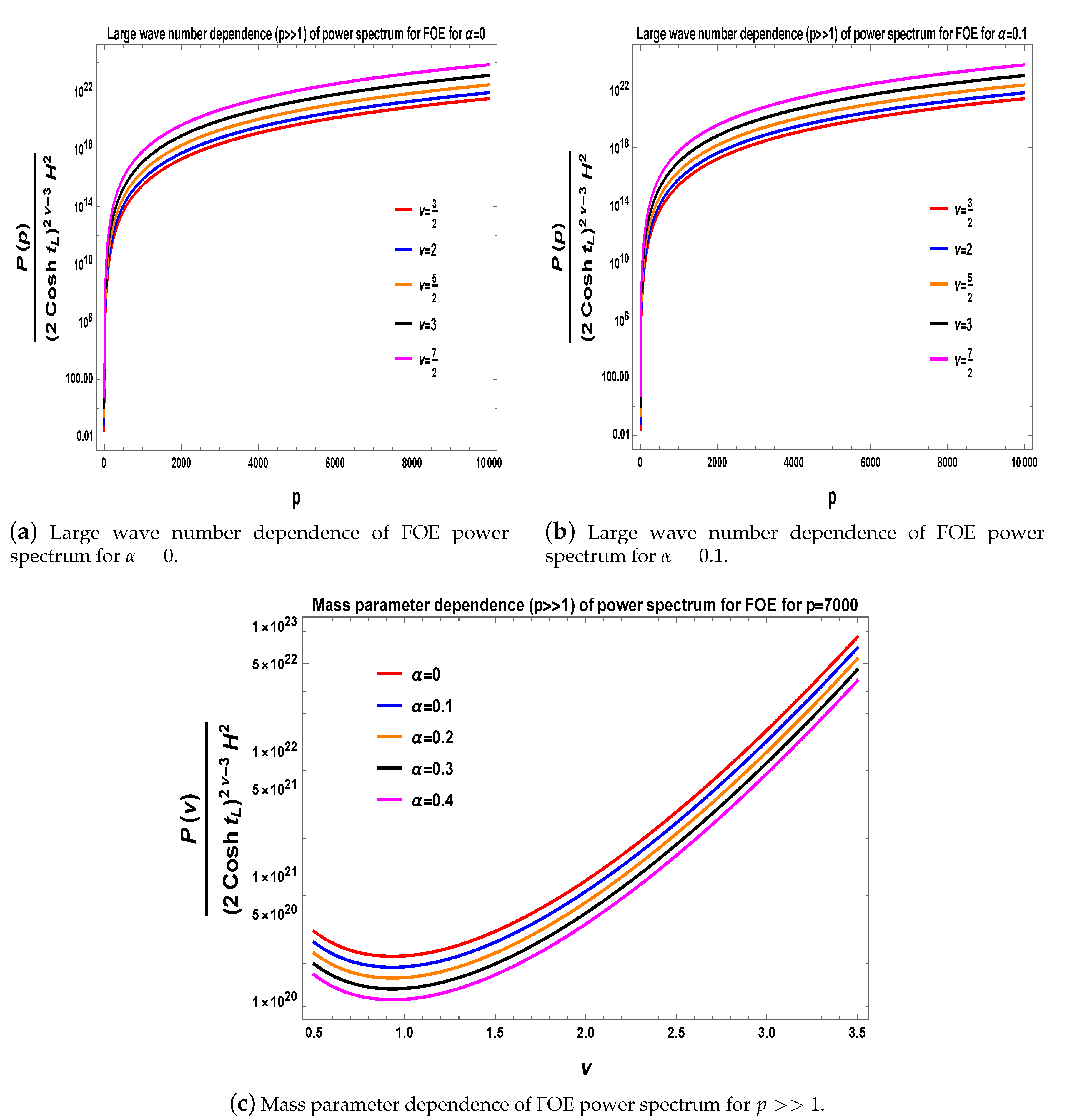
• In case of FOE formalism, we solve for the wave function in the region L and using this solution we compute the general expression for the mean square vacuum fluctuation and its quantum correction in terms of two point correlation function. The result is evaluated at all momentum scales. We considered two limiting approximation in the characteristic momentum scales, i.e., large wave number (small wave length in which the corresponding scale is smaller than the curvature radius of the de Sitter hyperbolic open chart) regime and small wave number (long wave length in which the corresponding scale is larger than the curvature radius of the de Sitter hyperbolic open chart) regime. We observed distinctive features in the power spectrum of of mean squared vacuum fluctuation in these two different regimes. In the large wave number (small wave length) regime we found that the leading order result for the power spectrum is consistent with the known result for observed cosmological correlation function in the super horizon time scale. The correction to the leading order result that we computed for the power spectrum can be interpreted as the sub-leading effect in the observed cosmological power spectrum. This is a strong information from the perspective of cosmological observation since such effects, possibly due to quantum entanglement of states, can play a big role to break the degeneracy of the observed cosmological power spectrum in the small wave length regime. On the other hand, in the long wave length regime we found that the power spectrum follows completely different momentum dependence in the super horizon time scale. Since in this regime and in this time scale, at present, we lack adequate observational data on power spectrum we are unable to comment on our result with observation. However, our result for the power spectrum in long wave length limit and super horizon time scale can be used as a theoretical probe to study the physical implications and its observational cosmological consequences in near future. Our result also implies that the mean square vacuum fluctuation for axion field, in super horizon time scale, gets enhanced in long wave length regime and freezes in the small wave length regime. We also observe that for a massive axion, the power spectrum is nearly scale invariant in all momentum scales. On the other hand, for massless axion we observe exact scale invariance only in large wave number (small wave length) regime and for the Bunch Davies initial quantum state. For generalised $\alpha$ initial state, we find slight modification in the corresponding power spectrum of the mean square vacuum fluctuation. The modification factor is proportional to $exp(-2\alpha )$ which is valid for all values of the parameter $\alpha$. It also implies that for large value of the parameter $\alpha$ we get additional exponential suppression for the power spectrum. This information can be used to distinguish between the role of Bunch Davies vacuum ($\alpha =0$) and any $\alpha$ vacua quantum initial state during analysis of observational data.
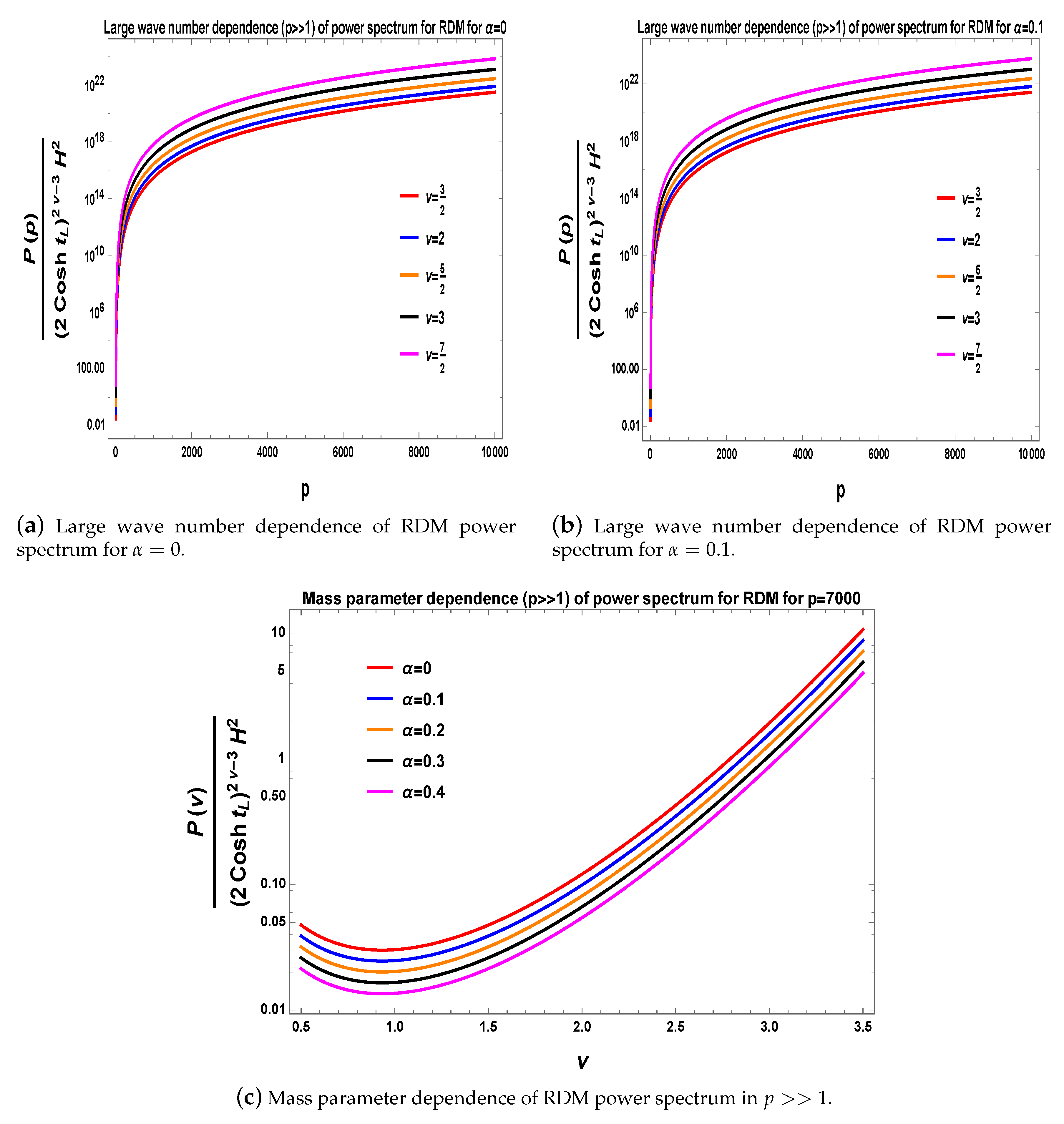
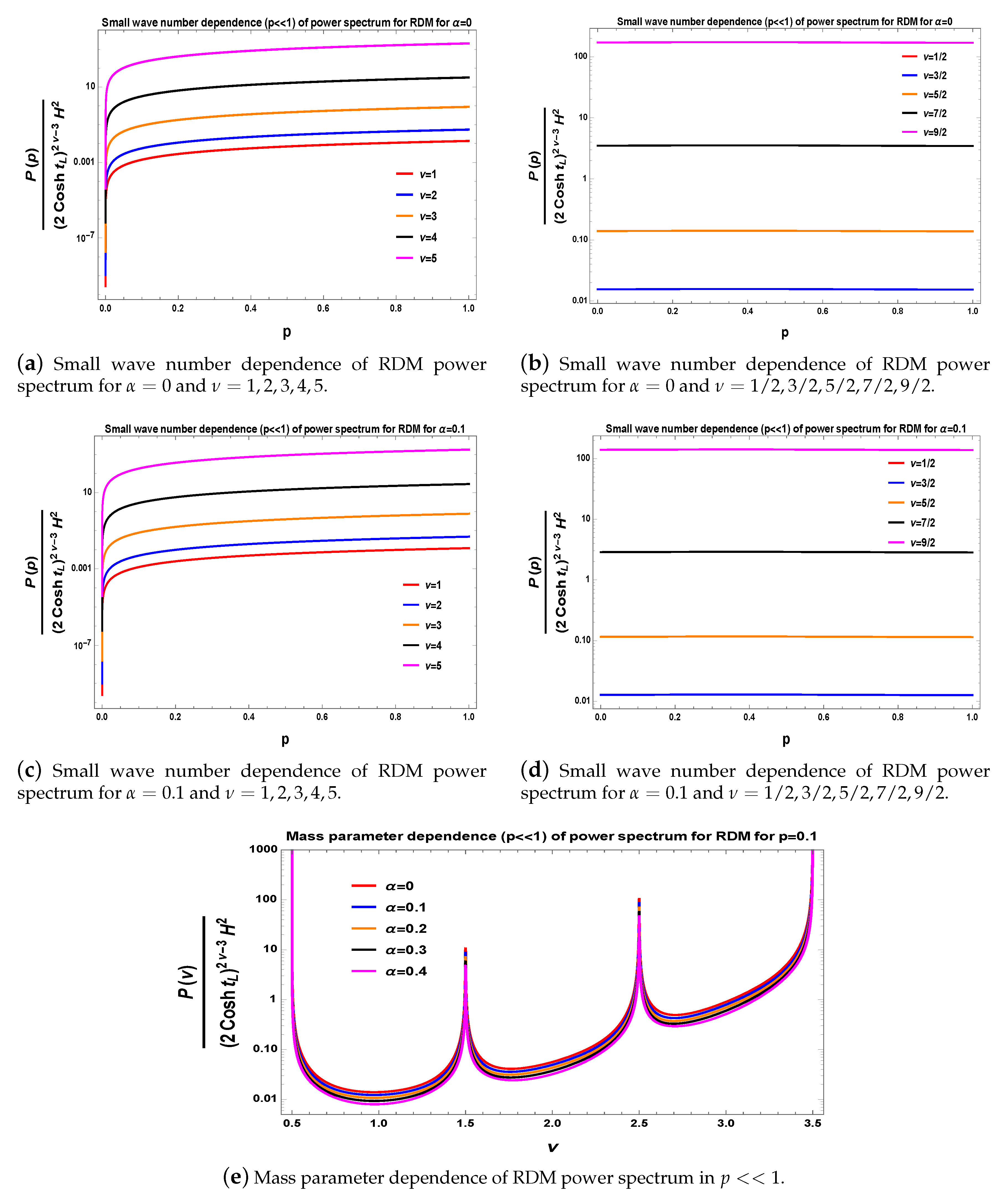
• In RDM formalism, the wave function for the axion field is solved in L and R regions of the de Sitter open chart. This solution was used to compute the mean square vacuum fluctuation and its quantum correction for both Bunch Davies and $\alpha$ vacuum state. Corresponding results are evaluated at all momentum scales by partially tracing out all the information from the region R. Like in the case of FOE, we considered the small and large wavelength approximations in the characteristic momentum scales and found distinct features in the corresponding power spectrum. In the small wave length regime again the leading order result, in super horizon time scales matched with known result (same as FOE). However, the sub-leading order result for the power spectrum is different from the result obtained from FOE formalism which distinguishes the two approaches. Moreover, in the long wave length regime the power spectrum has completely different momentum dependence compared to FOE formalism. We also noticed that the enhancement of mean square vacuum fluctuation for axion field, in long wave length regime, is different (slower) in nature compared to FOE formalism but the freezing in short wavelength regime is of same nature. The observation on scale invariance of power spectrum in this formalism remains similar to that in FOE formalism.
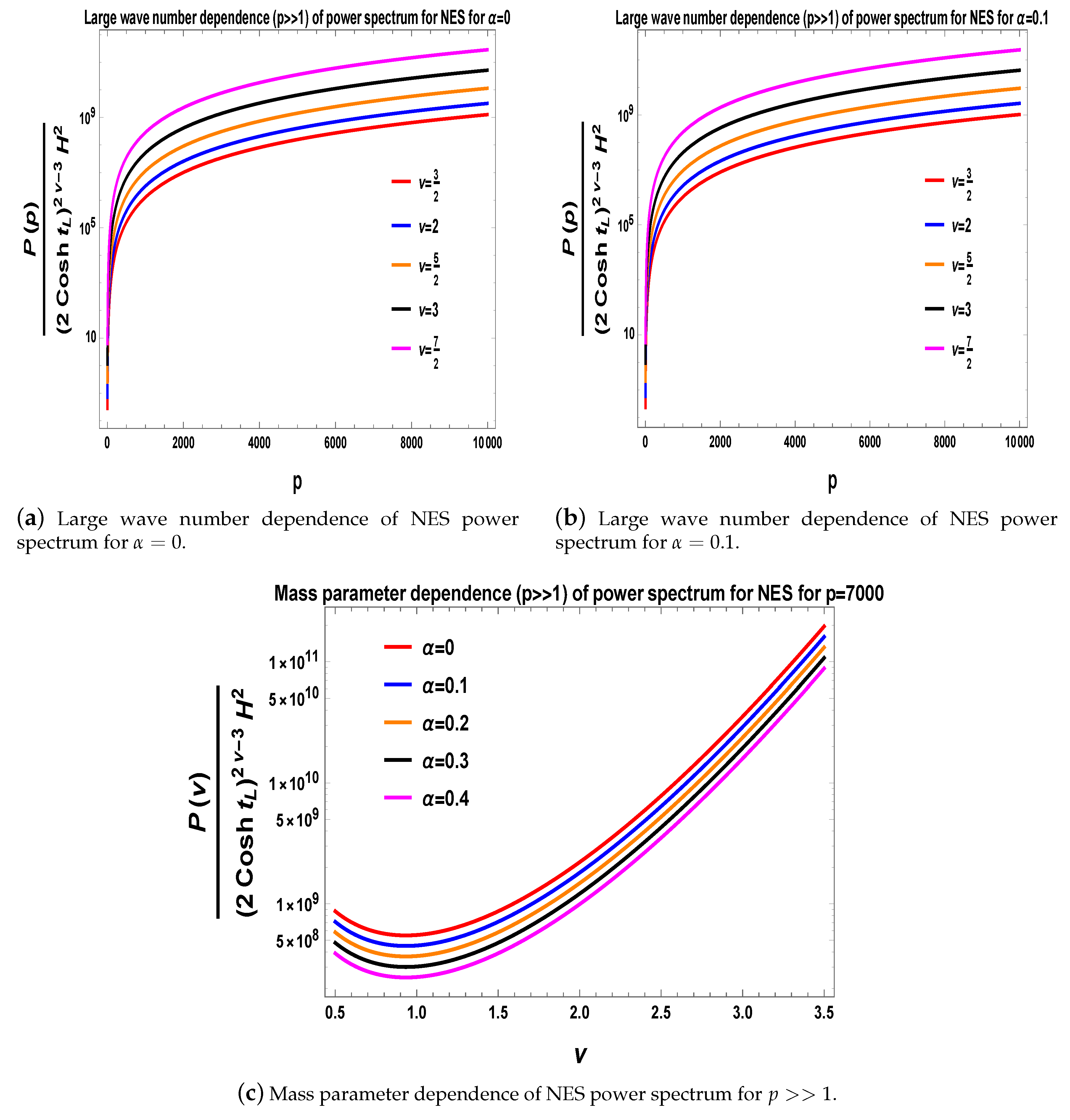
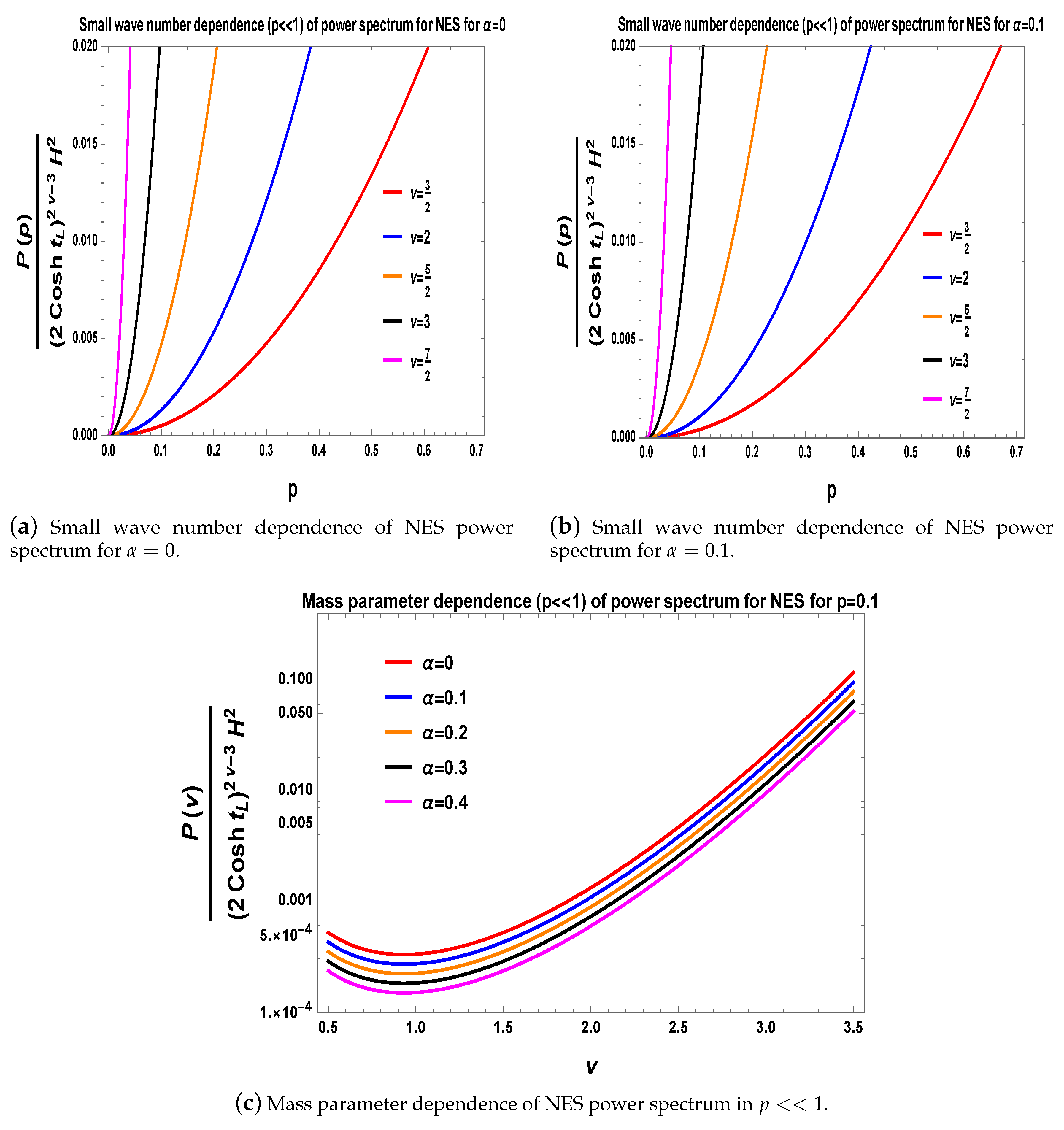
• In the last formalism, i.e., NES, the wave function of axion field is solved in the region L of the de Sitter hyperbolic open chart. With the help of this solution, t we computed the mean square vacuum fluctuation using Bunch Davies and $\alpha$ vacuum state configuration. The corresponding result is evaluated at all momentum scales. Like the previous two cases, here also we reverted to two limiting approximations, i.e., large wave number (small wave length ) regime and small wave number (long wave length) regime. We again observed distinctive behaviour in the power spectrum in these two different regimes. In the large wave number (small wave length) regime, the leading order result for power spectrum matches with the known result for observed cosmological correlation function just as the cases of FOE and RDM formalism. However, the sub-leading order result s completely different FOE as well as RDM formalism. Thus, it is the sub-leading terms which distinguish these formalisms from each other and they can be confronted with future observational data. On the other hand, in the small wave number (long wave length) regime, even the leading order result for the power spectrum differs, in momentum dependence, compared to the result obtained from FOE and RDM formalism. Also the nature of enhancement of the mean square vacuum fluctuation in NES formalism is found to be different from that in FOE and RDM formalism but the nature of freezing and the observation on scale invariance of power spectrum remains same in all the three cases.
• For completeness, we discuss the actual reason for the results obtained for the power spectra from quantum entangled state as appearing in FOE formalism and the mixed state which is used to construct the RDM formalism. To do so, we consider two subsystems, L and R using which one can construct the quantum mechanical state vector of axion field as ${|\mathsf{\Psi }\rangle }_{\mathbf{axion}}$. In our computation, these subsystems are defined in the region L and R respectively in the de Sitter hyperbolic open chart. Now using this state vector of axion field we can define the density matrix as:

  $${\rho }_{\mathbf{axion}}=|{\mathsf{\Psi }}_{\mathbf{axion}}\rangle \langle {\mathsf{\Psi }}_{\mathbf{axion}}|,$$

  (242)

  in both subsystems, L and R for FOE and RDM formalism and only the system L for NES formalism. Using this density matrix we can express the expectation value (for the total system) of a quantum mechanical operator ${\tilde{\mathcal{O}}}_{\mathbf{axion}}$, applicable for FOE and RDM formalism, as:

  $$\begin{array}{ccc}\mathbf{Tr}\left({\rho }_{\mathbf{axion}}{\tilde{\mathcal{O}}}_{\mathbf{axion}}\right)\hfill & =\hfill & {\sum }_{\mathbf{L}}{\sum }_{\mathbf{R}}\langle \mathbf{L},\mathbf{R}|{\mathsf{\Psi }}_{\mathbf{axion}}\rangle \langle {\mathsf{\Psi }}_{\mathbf{axion}}\left|{\tilde{\mathcal{O}}}_{\mathbf{axion}}\right|\mathbf{L},\mathbf{R}\rangle \hfill \\ \hfill & \equiv \hfill & \langle {\mathsf{\Psi }}_{\mathbf{axion}}\left|{\tilde{\mathcal{O}}}_{\mathbf{axion}}\right|{\mathsf{\Psi }}_{\mathbf{axion}}\rangle \hfill \\ \hfill & \equiv \hfill & \langle {\tilde{\mathcal{O}}}_{\mathbf{axion}}\rangle .\hfill \end{array}$$

  (243)

This is an important observation as it is related to the measurement and quantification of any physical cosmological observable in the quantum regime. However, in the case of NES formalism one can rewrite Equation (243) as:

$$\begin{array}{ccc}\mathbf{Tr}\left({\rho }_{\mathbf{axion}}{\tilde{\mathcal{O}}}_{\mathbf{axion}}\right)\hfill & =\hfill & {\sum }_{\mathbf{L}}{\sum }_{\mathbf{R}}\langle \mathbf{L},\mathbf{R}|{\mathsf{\Psi }}_{\mathbf{axion}}\rangle \langle {\mathsf{\Psi }}_{\mathbf{axion}}\left|{\tilde{\mathcal{O}}}_{\mathbf{axion}}\right|\mathbf{L},\mathbf{R}\rangle \hfill \\ \hfill & =\hfill & {\sum }_{\mathbf{L}}{\sum }_{\mathbf{R}}{\sum }_{{\mathbf{L}}^{{}^{\prime }}}{\sum }_{{\mathbf{R}}^{{}^{\prime }}}\langle \mathbf{L},\mathbf{R}|{\mathsf{\Psi }}_{\mathbf{axion}}\rangle \langle {\mathsf{\Psi }}_{\mathbf{axion}}|{\mathbf{L}}^{{}^{\prime }},{\mathbf{R}}^{{}^{\prime }}\rangle \langle {\mathbf{L}}^{{}^{\prime }},{\mathbf{R}}^{{}^{\prime }}\left|{\tilde{\mathcal{O}}}_{\mathbf{axion}}^{\mathbf{L}}\right|\mathbf{L},\mathbf{R}\rangle \hfill \\ \hfill & =\hfill & {\sum }_{\mathbf{L}}{\sum }_{\mathbf{R}}{\sum }_{{\mathbf{L}}^{{}^{\prime }}}{\sum }_{{\mathbf{R}}^{{}^{\prime }}}\langle \mathbf{L},\mathbf{R}|{\mathsf{\Psi }}_{\mathbf{axion}}\rangle \langle {\mathsf{\Psi }}_{\mathbf{axion}}|{\mathbf{L}}^{{}^{\prime }},{\mathbf{R}}^{{}^{\prime }}\rangle \langle {\mathbf{L}}^{{}^{\prime }}\left|{\tilde{\mathcal{O}}}_{\mathbf{axion}}^{\mathbf{L}}\right|\mathbf{L}\rangle {\delta }_{\mathbf{R}{\mathbf{R}}^{{}^{\prime }}}\hfill \\ \hfill & =\hfill & {\sum }_{\mathbf{L}}{\sum }_{\mathbf{R}}{\sum }_{{\mathbf{L}}^{{}^{\prime }}}\langle \mathbf{L},\mathbf{R}|{\mathsf{\Psi }}_{\mathbf{axion}}\rangle \langle {\mathsf{\Psi }}_{\mathbf{axion}}|{\mathbf{L}}^{{}^{\prime }},{\mathbf{R}}^{{}^{\prime }}\rangle \langle {\mathbf{L}}^{{}^{\prime }}\left|{\tilde{\mathcal{O}}}_{\mathbf{axion}}^{\mathbf{L}}\right|\mathbf{L}\rangle \hfill \\ \hfill & =\hfill & \mathbf{Tr}\left({\rho }_{\mathbf{axion}}^{\mathbf{L}}{\tilde{\mathcal{O}}}_{\mathbf{axion}}^{\mathbf{L}}\right),\hfill \end{array}$$

(244)

where the operator ${\tilde{\mathcal{O}}}_{\mathbf{axion}}^{\mathbf{L}}$ solely in the region L is defined by the following expression for NES formalism:

$$\begin{array}{ccc}\langle {\mathbf{L}}^{{}^{\prime }},{\mathbf{R}}^{{}^{\prime }}\left|{\tilde{\mathcal{O}}}_{\mathbf{axion}}^{\mathbf{L}}\right|\mathbf{L},\mathbf{R}\rangle \hfill & =\hfill & \langle {\mathbf{L}}^{{}^{\prime }}\left|{\tilde{\mathcal{O}}}_{\mathbf{axion}}^{\mathbf{L}}\right|\mathbf{L}\rangle \langle {\mathbf{R}}^{{}^{\prime }}|\mathbf{R}\rangle \hfill \\ \hfill & =\hfill & \langle {\mathbf{L}}^{{}^{\prime }}\left|{\tilde{\mathcal{O}}}_{\mathbf{axion}}^{\mathbf{L}}\right|\mathbf{L}\rangle {\delta }_{\mathbf{R}{\mathbf{R}}^{{}^{\prime }}}.\hfill \end{array}$$

(245)

Also in NES formalism the density matrix ${\rho }_{\mathbf{axion}}^{\mathbf{L}}$ for the region L is described by the following expression:

$$\begin{array}{ccc}{\rho }_{\mathbf{axion}}^{\mathbf{L}}\hfill & =\hfill & {\mathbf{Tr}}_{\mathbf{R}}{\rho }_{\mathbf{axion}}\hfill \\ \hfill & =\hfill & {\sum }_{\mathbf{L}}{\sum }_{{\mathbf{L}}^{{}^{\prime }}}|\mathbf{L}\rangle \left({\sum }_{\mathbf{R}}\langle \mathbf{L},\mathbf{R}|{\mathsf{\Psi }}_{\mathbf{axion}}\rangle \langle {\mathsf{\Psi }}_{\mathbf{axion}}|{\mathbf{L}}^{{}^{\prime }},{\mathbf{R}}^{{}^{\prime }}\rangle \right)\langle {\mathbf{L}}^{{}^{\prime }}|\hfill \\ \hfill & =\hfill & {\sum }_{\mathbf{L}}{\sum }_{{\mathbf{L}}^{{}^{\prime }}}|\mathbf{L}\rangle \left({\sum }_{\mathbf{R}}{\mathsf{\Psi }}_{\mathbf{axion}}(\mathbf{L},\mathbf{R}){\mathsf{\Psi }}_{\mathbf{axion}}^{*}({\mathbf{L}}^{{}^{\prime }},{\mathbf{R}}^{{}^{\prime }})\right)\langle {\mathbf{L}}^{{}^{\prime }}|.\hfill \end{array}$$

(246)

This implies that in NES formalism, the physical operator is solely described by the information from the region L and consequently the expectation value of such operator satisfy the following condition:

$$\begin{array}{ccc}\hfill \langle {\tilde{O}}_{\mathbf{axion}}\rangle =\mathbf{Tr}\left({\rho }_{\mathbf{axion}}{\tilde{\mathcal{O}}}_{\mathbf{axion}}\right)& =& \mathbf{Tr}\left({\rho }_{\mathbf{axion}}^{\mathbf{L}}{\tilde{\mathcal{O}}}_{\mathbf{axion}}^{\mathbf{L}}\right)=\langle {\tilde{O}}_{\mathbf{axion}}^{\mathbf{L}}\rangle .\hfill \end{array}$$

(247)

The above analysis can help us to explain the differences between the power spectra of mean square vacuum fluctuation obtained from FOE, RDM, and NES formalism on large scale (or small wave number or large wave length regime). It clearly points towards the fact that in FOE and RDM formalism the creation and annihilation operators for axion field includes new set of creation and annihilation operators coming from the Bogoliubov transformation from one quantum basis to the other. This means that the field operator in the FOE formalism also involves these extra creation and annihilation operators even if the computation is being performed on a particularly specified temporal slice defined in the region L of the Hilbert space. On the other hand, after applying the partial trace over the degrees of freedom from the region R, the mixed quantum state, using which we formulate the RDM formalism, is prepared by the creation and annihilation operators in the region L of the Hilbert space. Thus, in RDM formalism, the field operator is only defined in the region L and not in the region R of the Hilbert space. This implies that the field operator defined before partially tracing over the degrees of freedom from region R for FOE formalism is different from the field operator in region L used in RDM formalism since for this case we performed the partial trace over the degrees of freedom in region R. Thus, any general quantum mechanical operator defined in the framework of FOE is not same as that of RDM formalism.

Before we conclude, we point out that apart from the quantification of the mean square vacuum fluctuation in the formalisms we discussed here, we also computed the entanglement entropy using von Neumann measure and the Renyi entropy in our previous work [23,24].

References

- Horodecki, R.; Horodecki, P.; Horodecki, M.; Horodecki, K. Quantum entanglement. Rev. Mod. Phys. 2009, 81, 865. [Google Scholar] [CrossRef] [Green Version]
- Martin-Martinez, E.; Menicucci, N.C. Cosmological quantum entanglement. Class. Quantum Gravity 2012, 29, 224003. [Google Scholar] [CrossRef]
- Nambu, Y. Entanglement of Quantum Fluctuations in the Inflationary Universe. Phys. Rev. D 2008, 78, 044023. [Google Scholar] [CrossRef] [Green Version]
- Bell, J.S. On the Einstein-Podolsky-Rosen paradox. Physics 1964, 1, 195. [Google Scholar] [CrossRef] [Green Version]
- Coleman, S.R.; de Luccia, F. Gravitational Effects on and of Vacuum Decay. Phys. Rev. D 1980, 21, 3305. [Google Scholar] [CrossRef] [Green Version]
- Garriga, J.; Kanno, S.; Sasaki, M.; Soda, J.; Vilenkin, A. Observer dependence of bubble nucleation and Schwinger pair production. J. Cosmol. Astropart. Phys. 2012, 1212, 006. [Google Scholar] [CrossRef] [Green Version]
- Garriga, J.; Kanno, S.; Tanaka, T. Rest frame of bubble nucleation. J. Cosmol. Astropart. Phys. 2013, 1306, 034. [Google Scholar] [CrossRef]
- Fröb, M.B.; Garriga, J.; Kanno, S.; Sasaki, M.; Soda, J.; Tanaka, T.; Vilenkin, A. Schwinger effect in de Sitter space. J. Cosmol. Astropart. Phys. 2014, 1404, 009. [Google Scholar] [CrossRef] [Green Version]
- Fischler, W.; Nguyen, P.H.; Pedraza, J.F.; Tangarife, W. Holographic Schwinger effect in de Sitter space. Phys. Rev. D 2015, 91, 086015. [Google Scholar] [CrossRef] [Green Version]
- Laflorencie, N. Quantum entanglement in condensed matter systems. Phys. Rept. 2016, 646, 1. [Google Scholar] [CrossRef] [Green Version]
- Ryu, S.; Takayanagi, T. Holographic derivation of entanglement entropy from AdS/CFT. Phys. Rev. Lett. 2006, 96, 181602. [Google Scholar] [CrossRef] [PubMed] [Green Version]
- Takayanagi, T. Entanglement Entropy from a Holographic Viewpoint. Class. Quantum Gravity 2012, 29, 153001. [Google Scholar] [CrossRef] [Green Version]
- Ryu, S.; Takayanagi, T. Aspects of Holographic Entanglement Entropy. J. High Energy Phys. 2006, 0608, 045. [Google Scholar] [CrossRef] [Green Version]
- Nishioka, T.; Ryu, S.; Takayanagi, T. Holographic Entanglement Entropy: An Overview. J. Phys. A 2009, 42, 504008. [Google Scholar] [CrossRef] [Green Version]
- Rangamani, M.; Takayanagi, T. Holographic Entanglement Entropy. Lect. Notes Phys. 2017, 931. [Google Scholar]
- Hubeny, V.E.; Rangamani, M.; Takayanagi, T. A Covariant holographic entanglement entropy proposal. J. High Energy Phys. 2007, 0707, 062. [Google Scholar] [CrossRef]
- Maldacena, J.; Pimentel, G.L. Entanglement entropy in de Sitter space. J. High Energy Phys. 2013, 1302, 038. [Google Scholar] [CrossRef] [Green Version]
- Kanno, S.; Murugan, J.; Shock, J.P.; Soda, J. Entanglement entropy of α-vacua in de Sitter space. J. High Energy Phys. 2014, 1407, 072. [Google Scholar] [CrossRef] [Green Version]
- Allen, B. Vacuum States in de Sitter Space. Phys. Rev. D 1985, 32, 3136. [Google Scholar] [CrossRef] [Green Version]
- Goldstein, K.; Lowe, D.A. A Note on alpha vacua and interacting field theory in de Sitter space. Nucl. Phys. B 2003, 669, 325. [Google Scholar] [CrossRef] [Green Version]
- De Boer, J.; Jejjala, V.; Minic, D. Alpha-states in de Sitter space. Phys. Rev. D 2005, 71, 044013. [Google Scholar] [CrossRef] [Green Version]
- Brunetti, R.; Fredenhagen, K.; Hollands, S. A Remark on alpha vacua for quantum field theories on de Sitter space. J. High Energy Phys. 2005, 0505, 063. [Google Scholar] [CrossRef]
- Choudhury, S.; Panda, S. Entangled de Sitter from stringy axionic Bell pair I: An analysis using Bunch–Davies vacuum. Eur. Phys. J. C 2018, 78, 52. [Google Scholar] [CrossRef] [Green Version]
- Choudhury, S.; Panda, S. Quantum entanglement in de Sitter space from Stringy Axion: An analysis using α vacua. arXiv 2017, arXiv:1712.08299. [Google Scholar]
- Capolupo, A.; Lambiase, G.; Quaranta, A.; Giampaolo, S.M. Probing axion mediated fermion–fermion interaction by means of entanglement. Phys. Lett. B 2020, 804, 135407. [Google Scholar] [CrossRef]
- Patrascu, A.T. Axion mass and quantum information. Phys. Lett. B 2018, 786, 1–4. [Google Scholar] [CrossRef]
- Maldacena, J. A model with cosmological Bell inequalities. Fortsch. Phys. 2016, 64, 10. [Google Scholar] [CrossRef] [Green Version]
- Choudhury, S.; Panda, S.; Singh, R. Bell violation in the Sky. Eur. Phys. J. C 2017, 77, 60. [Google Scholar] [CrossRef]
- Choudhury, S.; Panda, S.; Singh, R. Bell violation in primordial cosmology. Universe 2017, 3, 13. [Google Scholar] [CrossRef] [Green Version]
- Kanno, S.; Soda, J. Infinite violation of Bell inequalities in inflation. arXiv 2017, arXiv:1705.06199. [Google Scholar]
- Panda, S.; Sumitomo, Y.; Trivedi, S.P. Axions as Quintessence in String Theory. Phys. Rev. D 2011, 83, 083506. [Google Scholar] [CrossRef] [Green Version]
- McAllister, L.; Silverstein, E.; Westphal, A. Gravity Waves and Linear Inflation from Axion Monodromy. Phys. Rev. D 2010, 82, 046003. [Google Scholar] [CrossRef] [Green Version]
- Silverstein, E.; Westphal, A. Monodromy in the CMB: Gravity Waves and String Inflation. Phys. Rev. D 2008, 78, 106003. [Google Scholar] [CrossRef] [Green Version]
- McAllister, L.; Silverstein, E.; Westphal, A.; Wrase, T. The Powers of Monodromy. J. High Energy Phys. 2014, 1409, 123. [Google Scholar] [CrossRef]
- Kanno, S. Impact of quantum entanglement on spectrum of cosmological fluctuations. J. Cosmol. Astropart. Phys. 2014, 1407, 029. [Google Scholar] [CrossRef] [Green Version]
- Kolevatov, R.; Mironov, S.; Rubakov, V.; Sukhov, N.; Volkova, V. Perturbations in generalized Galileon theories. Phys. Rev. D 2017, 96, 125012. [Google Scholar] [CrossRef] [Green Version]
- Libanov, M.; Mironov, S.; Rubakov, V. Generalized Galileons: Instabilities of bouncing and Genesis cosmologies and modified Genesis. J. Cosmol. Astropart. Phys. 2016, 1608, 037. [Google Scholar] [CrossRef]
- Libanov, M.; Rubakov, V.; Rubtsov, G. Towards conformal cosmology. JETP Lett. 2015, 102, 561. [Google Scholar] [CrossRef] [Green Version]
- Libanov, M.; Rubakov, V. Conformal Universe as false vacuum decay. Phys. Rev. D 2015, 91, 103515. [Google Scholar] [CrossRef] [Green Version]
- Libanov, M.; Rubakov, V.; Sibiryakov, S. TOn holography for (pseudo-)conformal cosmology. Phys. Lett. B 2015, 741, 239. [Google Scholar] [CrossRef] [Green Version]
- Rubakov, V.A. Cosmology. In Proceedings of the 2011 European School of High-Energy Physics (ESHEP 2011), Cheile Gradistei, Romania, 7–20 September 2011; pp. 151–195. [Google Scholar]
- Mironov, S.A.; Ramazanov, S.R.; Rubakov, V.A. Effect of intermediate Minkowskian evolution on CMB bispectrum. J. Cosmol. Astropart. Phys. 2014, 1404, 015. [Google Scholar] [CrossRef] [Green Version]
- Osipov, M.; Rubakov, V. Galileon bounce after ekpyrotic contraction. J. Cosmol. Astropart. Phys. 2013, 1311, 031. [Google Scholar] [CrossRef] [Green Version]
- Libanov, M.V.; Rubakov, V.A. Cosmological density perturbations in a conformal scalar field theory. Theor. Math. Phys. 2012, 170, 151. [Google Scholar] [CrossRef]
- Libanov, M.; Mironov, S.; Rubakov, V. Non-Gaussianity of scalar perturbations generated by conformal mechanisms. Phys. Rev. D 2011, 84, 083502. [Google Scholar] [CrossRef] [Green Version]
- Libanov, M.; Ramazanov, S.; Rubakov, V. Scalar perturbations in conformal rolling scenario with intermediate stage. J. Cosmol. Astropart. Phys. 2011, 1106, 010. [Google Scholar] [CrossRef] [Green Version]
- Libanov, M.; Rubakov, V. Cosmological density perturbations from conformal scalar field: Infrared properties and statistical anisotropy. J. Cosmol. Astropart. Phys. 2010, 1011, 045. [Google Scholar] [CrossRef] [Green Version]
- Osipov, M.; Rubakov, V. Scalar tilt from broken conformal invariance. JETP Lett. 2011, 93, 52. [Google Scholar]
- Rubakov, V.A. Harrison-Zeldovich spectrum from conformal invariance. J. Cosmol. Astropart. Phys. 2009, 0909, 030. [Google Scholar] [CrossRef] [Green Version]
- Libanov, M.V.; Rubakov, V.A. Lorentz-violating brane worlds and cosmological perturbations. Phys. Rev. D 2005, 72, 123503. [Google Scholar] [CrossRef] [Green Version]
- Rubakov, V.A. Relaxation of the cosmological constant at inflation? Phys. Rev. D 2000, 61, 061501. [Google Scholar] [CrossRef] [Green Version]
- Kopeikin, S.M.; Ramirez, J.; Mashhoon, B.; Sazhin, M.V. Cosmological perturbations: A New gauge invariant approach. Phys. Lett. A 2001, 292, 173. [Google Scholar] [CrossRef] [Green Version]
- Rubakov, V.A.; Sazhin, M.V.; Veryaskin, A.V. Graviton Creation in the Inflationary Universe and the Grand Unification Scale. Phys. Lett. 1982, 115B, 189. [Google Scholar] [CrossRef]
- Choudhury, S.; Panda, S. COSMOS-e′-GTachyon from string theory. Eur. Phys. J. C 2016, 76, 278. [Google Scholar] [CrossRef] [Green Version]
- Choudhury, S. COSMOS-e′- soft Higgsotic attractors. Eur. Phys. J. C 2017, 77, 469. [Google Scholar] [CrossRef] [Green Version]
- Choudhury, S.; Pal, S. Primordial non-Gaussian features from DBI Galileon inflation. Eur. Phys. J. C 2015, 75, 241. [Google Scholar] [CrossRef] [Green Version]
- Choudhury, S.; Pal, S. DBI Galileon inflation in background SUGRA. Nucl. Phys. B 2013, 874, 85. [Google Scholar] [CrossRef] [Green Version]
- Choudhury, S.; Pal, S. Fourth level MSSM inflation from new flat directions. J. Cosmol. Astropart. Phys. 2012, 1204, 018. [Google Scholar] [CrossRef]
- Choudhury, S.; Pal, S. Brane inflation in background supergravity. Phys. Rev. D 2012, 85, 043529. [Google Scholar] [CrossRef] [Green Version]
- Choudhury, S. Can Effective Field Theory of inflation generate large tensor-to-scalar ratio within Randall–Sundrum single braneworld? Nucl. Phys. B 2015, 894, 29. [Google Scholar] [CrossRef] [Green Version]
- Choudhury, S.; Pal, B.K.; Basu, B.; Bandyopadhyay, P. Quantum Gravity Effect in Torsion Driven Inflation and CP violation. J. High Energy Phys. 2015, 1510, 194. [Google Scholar] [CrossRef] [Green Version]
- Choudhury, S. Reconstructing inflationary paradigm within Effective Field Theory framework. Phys. Dark Univ. 2016, 11, 16. [Google Scholar] [CrossRef] [Green Version]
- Choudhury, S.; Mazumdar, A. An accurate bound on tensor-to-scalar ratio and the scale of inflation. Nucl. Phys. B 2014, 882, 386. [Google Scholar] [CrossRef] [Green Version]
- Choudhury, S.; Mazumdar, A. Primordial blackholes and gravitational waves for an inflection-point model of inflation. Phys. Lett. B 2014, 733, 270. [Google Scholar] [CrossRef] [Green Version]
- Choudhury, S.; Mazumdar, A. Reconstructing inflationary potential from BICEP2 and running of tensor modes. arXiv 2014, arXiv:1403.5549. [Google Scholar]
- Choudhury, S.; Mazumdar, A.; Pukartas, E. Constraining = 1 supergravity inflationary framework with non-minimal Kähler operators. J. High Energy Phys. 2014, 1404, 077. [Google Scholar] [CrossRef] [Green Version]
- Choudhury, S. Constraining = 1 supergravity inflation with non-minimal Kaehler operators using δN formalism. J. High Energy Phys. 2014, 1404, 105. [Google Scholar] [CrossRef] [Green Version]
- Choudhury, S.; Mazumdar, A.; Pal, S. Low & High scale MSSM inflation, gravitational waves and constraints from Planck. J. Cosmol. Astropart. Phys. 2013, 1307, 041. [Google Scholar]
- Choudhury, S. The Cosmological OTOC: Formulating new cosmological micro-canonical correlation functions for random chaotic fluctuations in Out-of-Equilibrium Quantum Statistical Field Theory. arXiv 2020, arXiv:2005.11750. [Google Scholar]
- Banerjee, S.; Choudhury, S.; Chowdhury, S.; Das, R.N.; Gupta, N.; Panda, S.; Swain, A. Indirect detection of Cosmological Constant from large N entangled open quantum system. arXiv 2020, arXiv:2004.13058. [Google Scholar]
- Akhtar, S.; Choudhury, S.; Chowdhury, S.; Goswami, D.; Panda, S.; Swain, A. Open Quantum Cosmology: A study of two body quantum entanglement in static patch of De Sitter space. arXiv 2019, arXiv:1908.09929. [Google Scholar]
- Bohra, H.; Choudhury, S.; Chauhan, P.; Mukherjee, A.; Narayan, P.; Panda, S.; Swain, A. Relating the curvature of De Sitter Universe to Open Quantum Lamb Shift Spectroscopy. arXiv 2019, arXiv:1905.07403. [Google Scholar]
- Choudhury, S.; Mukherjee, A. Quantum randomness in the Sky. Eur. Phys. J. C 2019, 79, 554. [Google Scholar] [CrossRef]
- Choudhury, S.; Mukherjee, A.; Chauhan, P.; Bhattacherjee, S. Quantum Out-of-Equilibrium Cosmology. Eur. Phys. J. C 2019, 79, 320. [Google Scholar] [CrossRef]
- Choudhury, S. Quantum Field Theory Approaches to Early Universe Cosmology; LAP Lambert Academic Publishing: Beau Bassin, Mauritius, 10 July 2018; ISBN -13: 978-6139840908. [Google Scholar]
- Maharana, J.; Mukherji, S.; Panda, S. Notes on axion, inflation and graceful exit in stringy cosmology. Mod. Phys. Lett. A 1997, 12, 447. [Google Scholar] [CrossRef] [Green Version]
- Mazumdar, A.; Panda, S.; Perez-Lorenzana, A. Assisted inflation via tachyon condensation. Nucl. Phys. B 2001, 614, 101. [Google Scholar] [CrossRef] [Green Version]
- Choudhury, D.; Ghoshal, D.; Jatkar, D.P.; Panda, S. Hybrid inflation and brane - anti-brane system. J. Cosmol. Astropart. Phys. 2003, 0307, 009. [Google Scholar] [CrossRef] [Green Version]
- Choudhury, D.; Ghoshal, D.; Jatkar, D.P.; Panda, S. On the cosmological relevance of the tachyon. Phys. Lett. B 2002, 544, 231. [Google Scholar] [CrossRef] [Green Version]
- Chingangbam, P.; Panda, S.; Deshamukhya, A. Non-minimally coupled tachyonic inflation in warped string background. J. High Energy Phys. 2005, 0502, 052. [Google Scholar] [CrossRef] [Green Version]
- Deshamukhya, A.; Panda, S. Warm tachyonic inflation in warped background. Int. J. Mod. Phys. D 2009, 18, 2093. [Google Scholar] [CrossRef] [Green Version]
- Moniz, P.V.; Panda, S.; Ward, J. Higher order corrections to Heterotic M-theory inflation. Class. Quantum Gravity 2009, 26, 245003. [Google Scholar] [CrossRef]
- Ali, A.; Deshamukhya, A.; Panda, S.; Sami, M. Inflation with improved D3-brane potential and the fine tunings associated with the model. Eur. Phys. J. C 2011, 71, 1672. [Google Scholar] [CrossRef] [Green Version]
- Bhattacharjee, A.; Deshamukhya, A.; Panda, S. A note on low energy effective theory of chromo-natural inflation in the light of BICEP2 results. Mod. Phys. Lett. A 2015, 30, 1550040. [Google Scholar] [CrossRef] [Green Version]
- Panda, S.; Sami, M.; Tsujikawa, S. Inflation and dark energy arising from geometrical tachyons. Phys. Rev. D 2006, 73, 023515. [Google Scholar] [CrossRef] [Green Version]
- Panda, S.; Sami, M.; Tsujikawa, S.; Ward, J. Inflation from D3-brane motion in the background of D5-branes. Phys. Rev. D 2006, 73, 083512. [Google Scholar] [CrossRef] [Green Version]
- Panda, S.; Sami, M.; Tsujikawa, S. Prospects of inflation in delicate D-brane cosmology. Phys. Rev. D 2007, 76, 103512. [Google Scholar] [CrossRef] [Green Version]
- Baumann, D. TASI lectures on Inflation 2009. arXiv 2009, arXiv:0907.5424. [Google Scholar]
- Baumann, D.; Dymarsky, A.; Klebanov, I.R.; McAllister, L. Towards an Explicit Model of D-brane Inflation. J. Cosmol. Astropart. Phys. 2008, 0801, 024. [Google Scholar] [CrossRef] [Green Version]
- Baumann, D.; McAllister, L. Advances in Inflation in String Theory. Ann. Rev. Nucl. Part. Sci. 2009, 59, 67. [Google Scholar] [CrossRef] [Green Version]
- Assassi, V.; Baumann, D.; Green, D. Symmetries and Loops in Inflation. J. High Energy Phys. 2013, 1302, 151. [Google Scholar] [CrossRef] [Green Version]
- Baumann, D.; McAllister, L. Inflation and String Theory, 1st ed.; Cambridge University Press: Cambridge, UK, 2015. [Google Scholar]
- Baumann, D.; Dymarsky, A.; Kachru, S.; Klebanov, I.R.; McAllister, L. Holographic Systematics of D-brane Inflation. J. High Energy Phys. 2009, 0903, 093. [Google Scholar] [CrossRef]
- Peiris, H.V.; Baumann, D.; Friedman, B.; Cooray, A. Phenomenology of D-Brane Inflation with General Speed of Sound. Phys. Rev. D 2007, 76, 103517. [Google Scholar] [CrossRef] [Green Version]
- Svrcek, P.; Witten, E. Axions In String Theory. J. High Energy Phys. 2006, 0606, 051. [Google Scholar] [CrossRef] [Green Version]