Conservation Laws and Travelling Wave Solutions for Double Dispersion Equations in (1+1) and (2+1) Dimensions


1
Departamento de Matemáticas, Universidad de Cádiz, P.O. Box 40, 11510 Puerto Real, Cádiz, Spain
2
International Institute for Symmetry Analysis and Mathematical Modelling, Department of Mathematical Sciences, North-West University, Mafikeng Campus, Private Bag X 2046, Mmabatho 2735, South Africa
3
College of Mathematics and Systems Science, Shandong University of Science and Technology, Qingdao 266590, Shandong, China
4
Department of Mathematics and Informatics, Azerbaijan University, Jeyhun Hajibeyli str., 71, AZ1007 Baku, Azerbaijan
*
Author to whom correspondence should be addressed.
Symmetry 2020, 12(6), 950; https://doi.org/10.3390/sym12060950
Submission received: 31 January 2020
/
Revised: 16 March 2020
/
Accepted: 18 March 2020
/
Published: 4 June 2020
(This article belongs to the Special Issue Conservation Laws and Symmetries of Differential Equations)
Abstract
:In this article, we investigate two types of double dispersion equations in two different dimensions, which arise in several physical applications. Double dispersion equations are derived to describe long nonlinear wave evolution in a thin hyperelastic rod. Firstly, we obtain conservation laws for both these equations. To do this, we employ the multiplier method, which is an efficient method to derive conservation laws as it does not require the PDEs to admit a variational principle. Secondly, we obtain travelling waves and line travelling waves for these two equations. In this process, the conservation laws are used to obtain a triple reduction. Finally, a line soliton solution is found for the double dispersion equation in two dimensions.
1. Introduction
In this work, we study two equations of double dispersion in one and two dimensions. The double dispersion (DD) equation arises in several physical applications. For instance, it is used in analyzing non-linear wave distribution in waveguide, interplay of waveguide and exterior medium, and, therefore, likelihood of energy interchange through lateral coverings of waveguide.
The author of [1] concentrated on the theory, generation, simulation, and propagation of strain solitary waves in a non-linearly elastic, straight cylindrical rod under finite distortions. For this, the general theory of wave propagation in non-linearly elastic solids was introduced, in which a new approach was developed to solve the corresponding DD equation with dissipative terms, which leads to new exact explicit solutions.
In physics of condensed matter, experiments dedicated to lucrative observation of solitary strain wave in solids are not mentioned. Undoubtedly, the description of long wave propagation in solids and liquids is to a certain extent analogous, which provides good estimate of soliton existence in solids [2].
Just after a forceful strain wave inseminates in the non-linearly bounded and elastic solid, curving of wave front can escalate swiftly up to changeless deformation appearance. This sensation could be evened alongside the dispersion of wave inside the wave guide [3,4,5].
In [6], the authors studied a multidimensional double dispersion equation
with , for , a real constant, or , . In [7], the authors investigated the Cauchy problem of Equation (1) and derived the existence (both locally and globally in time) and the blow-up of its solutions.
In this paper, we investigate Equation (1) for and .
The DD equation in dimensions is given by
which describes non-linear dispersive waves [1]. Here, is an arbitrary function of u and are real numbers.
The DD equation in two dimensions is of the form
where is an arbitrary function of u.
The Boussinesq equation reads
where is a constant. It arises in various physical applications. For example, it is used in the propagation of long waves in shallow water [8]. Researchers have developed many generalizations of Boussinesq equation. One of such generalizations is the modified Boussinesq equation. In [9], generalization of Equation (4) of the form
was studied and classical and nonclassical symmetries were investigated in [10]. Here, is an arbitrary function of u.
Conservation laws have various utilizations in investigation of PDEs, for instance the determination of conserved quantities and also the constants of motion. These can also be applied to identify integrability and linearization and moreover in verifying the correctness of numerical methods.
The celebrated theorem by Noether [11] can be used to derive conservation laws for variational problems. For any PDE, whether it comes from variational problem or non-variational problem, conservation laws can be determined by a direct method [12,13,14,15,16].
Recently, double reduction of PDEs was performed by using the interrelation between symmetries and conservation laws [17,18,19]. Lately, non-linear power generalizations of the Kadomtsev–Petviashvili and Boussinesq equations were studied and line soliton solutions were constructed for [20].
This paper is arranged as follows: In Section 3 and Section 4, conservations laws for the double dispersion Equations (2) and (3) are obtained, respectively. Finally, travelling waves , are, respectively, determined for DD Equations (2) and (3), where determines direction and represents speed of travelling wave. The associated fourth-order non-linear ODEs for U are reduced to first-order variables separable equations by the application of conservation laws derived here for DD equations.
2. Lie Symmetries
Symmetries are a basic structure of nonlinear PDEs and they can be used to find invariant solutions and yield transformations that map the set of solutions into itself. A general discussion of symmetries and their applications to differential equations can be found in Refs. [15,21,22].
To apply the Lie symmetry method to Equation (3), we consider a one-parameter Lie group of infinitesimal transformations on :
where is the group parameter. For this transformation to be a symmetry, it must leave invariant the set of solutions of Equation (3). This invariance condition yields an overdetermined linear system of equations for the infinitesimals , , , and . Each set of infinitesimals corresponds to an infinitesimal symmetry with the generator
The symmetry generator can be used to find invariant solutions of Equation (3) determined by solving the invariant surface condition whose form is
We write the point symmetries admitted by the DD equation in (2+1) dimensions in Equation (3) in Table 1.
We point out that, for , Lie classical symmetries were derived for the DD equation in (1+1) dimensions (1.2) in [10], where, for , Equation (1.2) only admits translations in t and x.
3. Conservation Laws for DD Equation in (1+1) Dimension
We obtain conservation laws for DD Equation (2) by using the general multiplier method [12,13,14,22]. We recall that a conservation law for Equation (2) is a continuity equation
that holds for all solutions of Equation (2). is called a conserved current, where T is the conserved density and X is the spatial flux. Both are functions of t, x, and u and derivatives of u [21]. The operators and are the usual total derivative operators [15].
Two conservation laws are equivalent [22] provided they vary by a trivial conservation law , . Here, T and X are calculated on solutions of Equation (2), and is some function which depends on t, x, and u and derivatives of u.
Firstly, we note that Equation (2) has a Cauchy–Kovalevskaya form, which tells us that all non-trivial conservation laws arise from multipliers [13,14]. Especially, when one moves off of the solution set of Equation (2), every non-trivial conservation law in Equation (9) is identical to one that can be expressed as
where is a conservation law multiplier, and and vary from by a trivial conserved current. On the solutions set of Equation (2), the characteristic form in Equation (10) curtails to the conservation law in Equation (9).
For our problem, the determining equation for determining all multipliers is
which must hold off of the solutions set of Equation (2). As soon as the multipliers are determined, the associated non-trivial conservation laws are derived using a homotopy formula [12,13,14] or else by integrating Equation (10) [21].
We look for low-order multipliers [19,22] as these provide us with physically interesting conservation laws. The determining Equation (11) splits with respect to the remaining variables. We use Maple to solve the determining system with the conditions that , and .
This classification yields the following four cases:
- Case 1: . This case gives the following corresponding conserved density and flux:
- Case 2: . For this case, we obtain conserved density and flux as
- Case 3: . We get conserved density and flux as
- Case 4: . For this last case, the corresponding conserved density and flux are
4. Conservation Laws for DD Equation in (2+1) Dimension
For the (2+1) dimensions Equation (3), a local conservation law is the continuity equation
which holds for all solutions of Equation (3). Here, as before, T is conserved density and X and Y are spatial fluxes. Thus, every conservation law can be expressed as
In this case, we seek low order multipliers (as these are physically interesting), namely . Consequently, the determining equation is given by
Here,
is the Euler operator [15,21,22]. The determining equation, after splitting, yields (with and ):
Using Maple, we obtain the following eight cases. In each case, we provide the multiplier and corresponding low-order conservation law.
- Case 1: For ,
- Case 2: For ,
- Case 3: For ,
- Case 4: For ,
- Case 5: For ,
- Case 6: For ,
- Case 7: For ,
- Case 8: For ,
5. Travelling Waves for Equations (2) and (3)
In this section, we present travelling waves solutions for the DD Equations (2) in one dimension and line travelling waves for the DD Equation (3) in two dimensions. It is common knowledge that, if a differential equation has a Noether symmetry, then corresponding to this symmetry there exists a conservation law and moreover a double reduction can be performed on the differential equation [15,17]. For instance, in [17,18,19], the connection between symmetries and conservation laws was utilized to perform double reduction of PDEs.
In [19,23], an association between symmetries and conservation laws was further explored by concentrating on conservation laws which were invariant under a given set of symmetries. Furthermore, a few applications of determining symmetry-invariant conservation laws and determining symmetry-invariant solutions of PDEs were presented.
5.1. The (1+1)-DD Travelling Waves
We derive travelling waves for Equation (2) and use the travelling wave variable, namely . A travelling wave solution is of the form
and substituting this expression into Equation (2), we get the reduced nonlinear fourth-order ODE
We observe that these travelling wave solutions arise from invariance under the translation symmetry
Suppose a conservation law does not contain the variables t and x explicitly. Then, it gives rise to a reduction of order of travelling wave ODE by the reductions
yielding
Thus, the first integral is
and the corresponding symmetry-invariant conservation law is the first integral of Equation (32) as does not contain the variables t and x explicitly. Then, the conservation law gives rise to a first integral that yields the following reduced form of the travelling wave ODE
Moreover, although conservations laws and contain explicitly the variables x and t, however, the linear combination
is invariant under the generator , yielding a functionally independent second first integral
5.2. The (2+1)-DD Line Travelling Waves
In [20], line soliton solutions of generalized KP and Boussinesq equations with p-power nonlinearities in two dimensions were derived. In [24], line soliton solutions were derived for a family of modified KP equations, whereas, in [25], line soliton solutions were constructed for a family of modified KP equations with p-power nonlinearities. In [26], the authors derived conserved vectors for a double dispersion equation.
We now derive the explicit line travelling waves for Equation (3) and use the travelling wave variable for this derivation. A line travelling wave in two-dimensions is
The substitution of Equation (39) into Equation (3) gives the fourth-order non-linear DE for , namely
We observe that a travelling wave solution remains invariant with respect to three-parameter group of translations, namely , , , with .
Assume that a conservation law does not contain the variables t, x, and y explicitly. Subsequently, the conservation law gives rise to a reduction of order of travelling wave ODE by the reductions
yielding
Thus, the first integral is given by
and the corresponding symmetry-invariant conservation law will be a first integral of Equation (40) as that does not contain t, x, and y explicitly. Hence, the conservation law gives rise to the following reduction of order of travelling wave ODE:
Moreover, although conservations laws , , and contain explicitly the variables x, y, and t. However, the linear combination
is invariant under the generator yielding a second functionally independent first integral
Setting , we get a separable ODE that can be integrated once, yielding the following first-order ODE:
We remark that the double reduction method applied to a fourth-order PDE yields one third-order ODE, while we are getting a triple reduction to a second-order ODE [14].
6. Conclusions
In this paper, we study the (1+1)-dimensional and (2+1)-dimensional double dispersion equations, namely Equations (2) and (3). Firstly, we determine all low-order conservation laws by using the multiplier method for Equations (2) and (3). For the double dispersion Equation (2), we obtain four multipliers and, consequently, four conserved densities and fluxes are constructed. On the other hand, the double dispersion Equation (3) provides eight multipliers, which result in eight low-order conservation laws. Secondly, we derive the symmetry invariant conservation laws. In the case of translation symmetries, we show how conservation laws that explicitly contain the independent variables can nevertheless be used to obtain a triple reduction. This is done by obtaining two functionally independent first integrals yielding to a first-order ODE, which gives rise to travelling wave solutions. In particular, we find a line soliton solution for Equation (3).
Author Contributions
All authors made an equal contribution to the preparing the manuscript. All authors have read and agreed to the published version of the manuscript.
Acknowledgments
The authors warmly thank S. Anco for his help. The support of Junta de Andalucía FQM-201 group and University of Cádiz is gratefully acknowledged. CMK thanks North-West University for its continued support.
Conflicts of Interest
The authors declare no conflict of interest.
References
- Samsonov, A.M. Strain Solitons in Solids and How to Construct Them; Chapmanan d Hall: BocaRaton, FL, USA, 2001. [Google Scholar] [CrossRef]
- Bell, J.F. Experimental foundation of solid mechanics. In Encyclopaedia of Physics; Truesdell, C., Ed.; Springer: Berlin, Germany, 1973. [Google Scholar]
- Samsonov, A.M. Structural optimization in nonlinear elastic wave propagation problems. In Structural Optimization Under Dynamical Loading; Seminar andWorkshop of Junior Scientists; Lepik, U., Ed.; Tartu University Press: Tartu, Estonia, 1982; pp. 75–76. [Google Scholar]
- Samsonov, A.M. Soliton evolution in a rod with variable cross section. Sov. Phys. Dokl. 1984, 29, 586–587. [Google Scholar]
- Samsonov, A.M. Nonlinear strain waves in elastic waveguides. In Nonlinear Waves in Solids; Jeffrey, A., Engelbrecht, J., Eds.; Nonlinear Waves in Solids, CISM Courses and Lectures (International Centre for Mechanical Sciences); Springer: Vienna, Austria, 1994; Volume 341, pp. 349–382. [Google Scholar]
- Yu, J.; Li, F.; She, L. Lie Symmetry Reductions and Exact Solutions of a Multidimensional Double Dispersion Equation. Appl. Math. 2017, 8, 712–723. [Google Scholar] [CrossRef] [Green Version]
- Polat, N.; Ertas, A. Existence and Blow-Up of Solution of Cauchy Problem for the Generalized Damped Multidimensional Boussinesq Equation. J. Math. Anal. Appl. 2009, 349, 10–20. [Google Scholar] [CrossRef] [Green Version]
- Boussinesq, J. Théorie des ondes et des remous qui se propagent le long d’ un canal rectangulaire horizontal en communiquant au liquide contenudans ce canal des vitesses sensiblement pareilles de la surface au fond. J. Math. Pures Appl. 1872, 17, 55–108. [Google Scholar]
- Liu, Y. Instability and blow-up of solutions to a generalized Boussinesq equation. SIAM J. Math. Anal. 1995, 26, 1527–1546. [Google Scholar] [CrossRef]
- Gandarias, M.L.; Bruzón, M.S. Classical and Nonclassical Symmetries of a Generalized Boussinesq Equation. J. Nonlinear Math. Phys. 1998, 5, 8–12. [Google Scholar] [CrossRef] [Green Version]
- Noether, E. Invariante Variationsprobleme, Nachrichten von der Königlichen. Gesellschaft der Wissenschaften zu Göttingen. 1918, pp. 234–257. Available online: https://eudml.org/doc/59024 (accessed on 30 January 2020).
- Anco, S.C.; Bluman, G. Direct Construction of Conservation Laws from Field Equations. Phys. Rev. Lett. 1997, 78, 2869–2873. [Google Scholar] [CrossRef]
- Anco, S.C.; Bluman, G. Direct constrution method for conservation laws for partial differential equations Part I: Examples of conservation law classifications. Eur. J. Appl. Math. 2002, 13, 545–566. [Google Scholar] [CrossRef] [Green Version]
- Anco, S.C.; Bluman, G. Direct constrution method for conservation laws for partial differential equations Part II: General treatment. Eur. J. Appl. Math. 2002, 41, 567–585. [Google Scholar] [CrossRef] [Green Version]
- Olver, P.J. Applications of Lie Groups to Differential Equations; Springer: Berlin, Germany, 1986. [Google Scholar]
- Bluman, G.W.; Kumei, S. Symmetries and Differential Equations; Springer: Berlin, Germany, 1989. [Google Scholar]
- Sjöberg, A. Double reduction of PDEs from the association of symmetries with conservation laws with applications. Appl. Math. Comput. 2007, 184, 608–616. [Google Scholar] [CrossRef]
- Kara, A.H.; Mahomed, F.M. Relationship between symmetries and conservation laws. Int. J. Theor. Phys. 2000, 39, 23–40. [Google Scholar] [CrossRef]
- Anco, S.C. Symmetry properties of conservation laws. Int. J. Mod. Phys. B 2016, 30, 1640003. [Google Scholar] [CrossRef] [Green Version]
- Anco, S.C.; Gandarias, M.L.; Recio, E. Conservation laws, symmetries, and line soliton solutions of generalized KP and Boussinesq equations with p-power nonlinearities in two dimensions. Theor. Math. Phys. 2018, 197, 1393–1411. [Google Scholar] [CrossRef] [Green Version]
- Bluman, G.; Cheviakov, A.F.; Anco, S.C. Applications of Symmetry Methods to Partial Differential Equations; Springer: Berlin, Germany, 2010; pp. 119–182. [Google Scholar]
- Anco, S.C. Generalization of Noether’s theorem in modern form to non-variational partial differential equations. In Recent Progress and Modern Challenges in Applied Mathematics, Modeling and Computational Science; Springer: Berlin, Germany, 2017; pp. 119–182. [Google Scholar]
- Anco, S.C.; Kara, A.H. Symmetry invariance of conservation laws of partial differential equations. Eur. J. Appl. Math. 2018, 29, 78–117. [Google Scholar] [CrossRef]
- Anco, S.C.; Gandarias, M.L.; Recio, E. Conservation laws and line soliton solutions of a family of modified KP equations. Discret. Contin. Dyn. Syst. S 2019. [Google Scholar] [CrossRef] [Green Version]
- Anco, S.C.; Gandarias, M.L.; Recio, E. Line solitons and conservation laws of a modified KP equation with p-power nonlinearities. arXiv 2019, arXiv:1908.03962. [Google Scholar]
- Gandarias, M.L.; Khalique, M.C. Conserved vectors for a double dispersion equation. AIP Conf. Proc. 2019, 2116, 190002. [Google Scholar] [CrossRef]
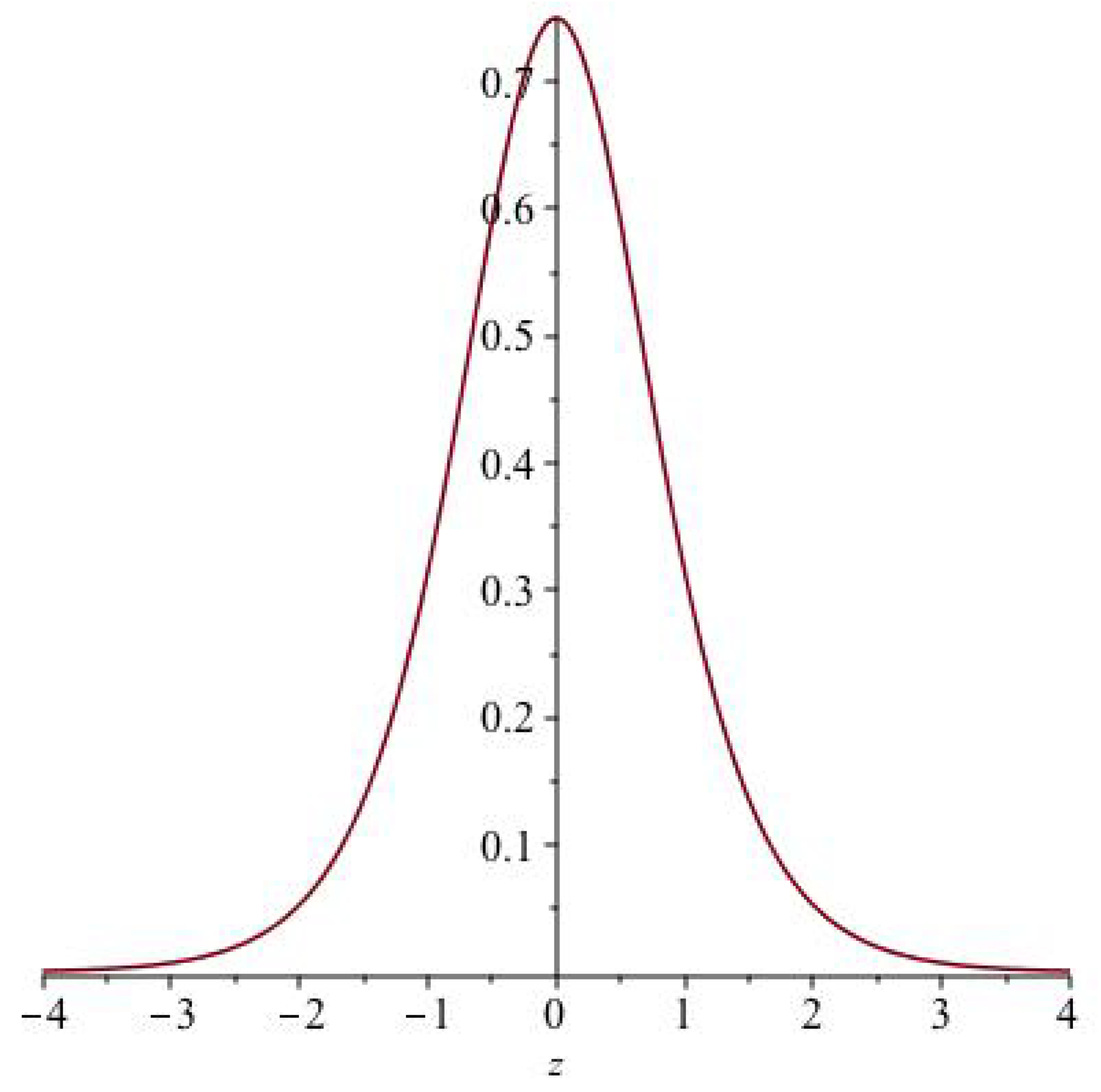
Figure 1.
Plot of solution for Equation (46).
Figure 1.
Plot of solution for Equation (46).


Table 1.
Point symmetries admitted by the DD equation in (2+1) dimensions.
| i | a | b | f(u) | |
|---|---|---|---|---|
| 1 | ||||
| 2 | 0 | |||
| 3 | 0 | |||
| 4 | 0 | |||
| 5 | 0 |
© 2020 by the authors. Licensee MDPI, Basel, Switzerland. This article is an open access article distributed under the terms and conditions of the Creative Commons Attribution (CC BY) license (http://creativecommons.org/licenses/by/4.0/).
Share and Cite
MDPI and ACS Style
Gandarias, M.L.; Durán, M.R.; Khalique, C.M. Conservation Laws and Travelling Wave Solutions for Double Dispersion Equations in (1+1) and (2+1) Dimensions. Symmetry 2020, 12, 950. https://doi.org/10.3390/sym12060950
AMA Style
Gandarias ML, Durán MR, Khalique CM. Conservation Laws and Travelling Wave Solutions for Double Dispersion Equations in (1+1) and (2+1) Dimensions. Symmetry. 2020; 12(6):950. https://doi.org/10.3390/sym12060950
Chicago/Turabian StyleGandarias, María Luz, María Rosa Durán, and Chaudry Masood Khalique. 2020. "Conservation Laws and Travelling Wave Solutions for Double Dispersion Equations in (1+1) and (2+1) Dimensions" Symmetry 12, no. 6: 950. https://doi.org/10.3390/sym12060950
Note that from the first issue of 2016, this journal uses article numbers instead of page numbers. See further details here.