Function Reconstruction from Reflection Symmetric Radon Data


Laboratoire de Physique Théorique et Modélisation, UMR 8089 CNRS/CY Cergy Paris Université, 95302 Cergy-Pontoise CEDEX, France
Symmetry 2020, 12(6), 956; https://doi.org/10.3390/sym12060956
Submission received: 2 April 2020
/
Revised: 1 May 2020
/
Accepted: 6 May 2020
/
Published: 4 June 2020
(This article belongs to the Special Issue Symmetry and Symmetry Breaking: Phase Transitions and Critical Phenomena)
Abstract
:In many areas of two-dimensional imaging science, data acquisition arises as an integral process. The inverse process—or image reconstruction—means the solving of a Radon problem mathematically. It may happen that there exists classes of integral data which are mirror symmetric with respect to a line. Common sense suggests that the occurrence of a symmetry usually provides significant help in the search of the problem solution. Here, we showed an example of the contrary to this popular belief. In fact, to solve such a Radon problem with inherent reflection symmetry, there is a need to split it into two new Radon problems on half-spaces, which do not have solutions at hand. In this paper, a full solution is obtained via geometric inversion mapping of the two original half-spaces Radon problems to the disk interior/exterior Radon problem arising in recent modalities of Compton scattering tomography, which fortunately has explicit worked out inverse formulas.
1. Introduction
By definition, the Radon problem, which arises for example in radiation imaging processes, is an inverse problem which consists of reconstructing a function from its integrals over a set of manifolds in space. Here, we shall limit ourselves to the Euclidean plane , in which the manifolds are smooth curves. Radon had considered first straight lines as smooth curves, and his work has found a successful imaging application in the so-called Computed Tomography (CT). As a natural next step, one would expect circles (or circular arcs) of the plane to come up in some generalized Radon transforms which are possibly linked to some new imaging processes. As a circle has more parameters than a line, there are many possible classes of Radon transforms defined on circles of the plane. As examples one may cite the following Radon transforms.
(a) In Compton Scatter Tomography (CST), where the acquired data consists of integrals of the electric charge density of the object under study on three distinct families of circular arcs, see, e.g., in [1].
(b) In Photoacoustic Tomography (PAT) or Thermoacoustic Tomography (TAT), where the acquired data consists of integral of the acoustic signal over circles (or circular arcs) centered on a fixed circle, see [2,3].
Let us now consider circles of example (b). These circles, which are centered on a fixed circle, do not display any particular symmetry. However, when the radius of the fixed circle goes to infinity, the set of circles, which are centered now on a fixed line, are now obviously symmetric with respect to this fixed line. Therefore, the corresponding integral data (or Radon data) is also reflection symmetric. This property introduces an ambiguity which does not allow to get a full solution of this Radon problem, as we shall see.
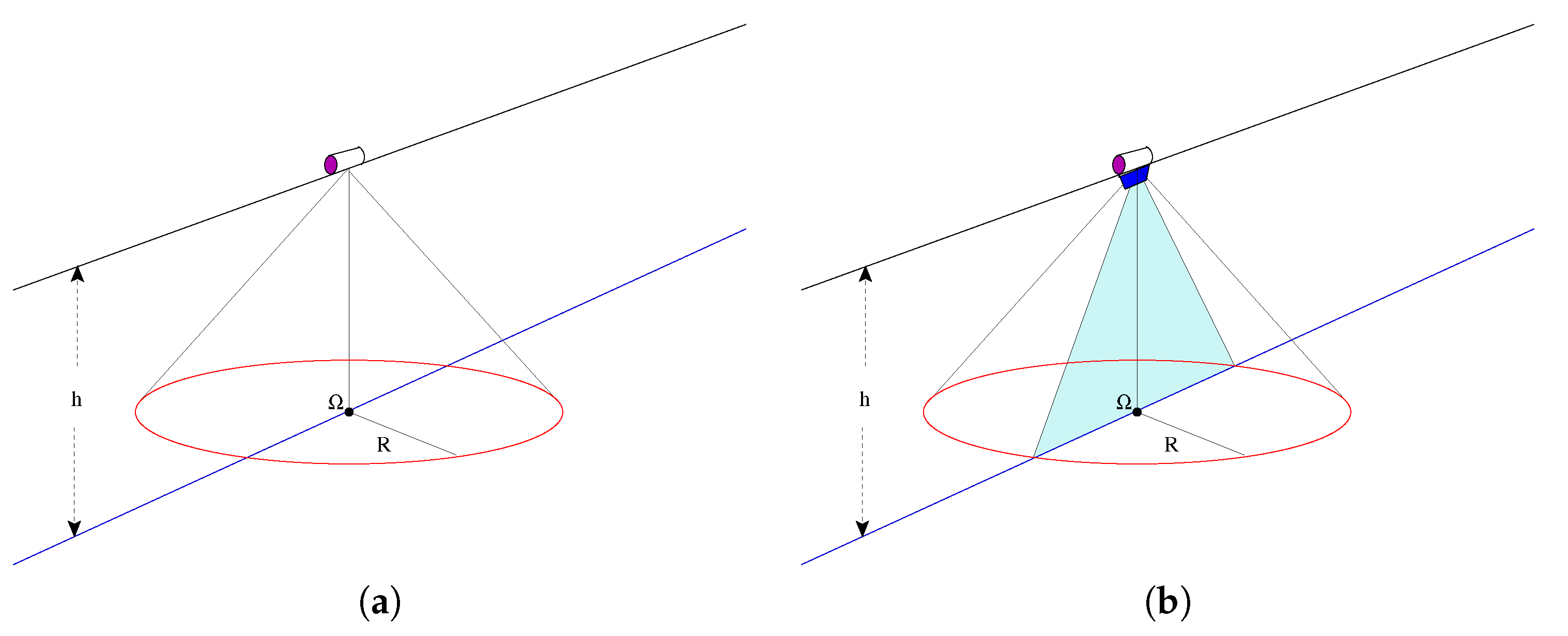
Such a situation has actually occurred in the historical development of Synthetic Antenna Radar (SAR) imaging. From 1985 to 2005, the idea of treating SAR imaging as a Radon problem was originally advocated by Hellsten and Andersson in [4]. They have considered that the received electromagnetic signal, by a monostatic radar antenna on a platform moving parallel to the ground at a given height h, is essentially the integral of the mean ground reflectivity over a set of circles centered on a fixed straight line (see their Equation (2.3) in [4]). Let us review briefly the main ideas in this proposition. The wavefront emanating from the emitting radar antenna is spherical and centered at this antenna. Consider now a planar terrain to be imaged. This wave front will impinged the terrain at half travel time before being registered back at the antenna (which is now on detection mode). Ignoring the effects of shape and duration of the transmitted pulse, the registered radiation pulse represents an average of the ground reflectivity function at the emitted radiation frequency or the integral of this function on a circle, which is the intersection of the emitted spherical wavefront with the planar terrain. Of course the center of this circle is on the vertical projection of the flight path of the antenna and its radius depends on the so-called fast time, which is the time interval between transmission and reception of a pulse. The recorded data clearly depends also on the position of the radar antenna on its flight path or equivalently on the position of the circle center on its linear path on the ground, which is now function of the so-called slow time in this data gathering process. This is schematically shown by the left image of Figure 1. The question is now how to extract from the acquired integral data.
An approximate reconstruction of the unknown function was worked out by Hellsten and Andersson in [4], in which proper features and issues of SAR imaging have been taken into account, yet under the assumption that is symmetric with respect to the line of circle centers, as in [5,6,7]. A few years later, Rothaus, well aware of the ambiguity caused by the reflection symmetric data, proposed a resolution method, which amounts to solving the new Radon problem on a half-plane, also identified to the Poincaré plane. His answer to this problem is an extension of Radon’s original inversion formula to this Poincaré plane [8], which is quite unwieldy for practical use. In 1997, Lindberg, while working towards a thesis, has pointed out that the ambiguity problem can be in principle resolved by adopting a double symmetric separate side scans in [9], as pictured by the right image of Figure 1 (see Section The CARABAS geometry in [9]). His proposal amounts to split up the original Radon problem (with its inherent reflection symmetry ambiguity) into two new Radon transforms on semi-circles centered on the line boundary of two half planes. This type of problem was precisely solved by Palamodov in 2000 [10], using high-level complex analysis transformations. Curiously, Palamodov had cited an application of his results to seismics instead to SAR. In this paper, we undertake to achieve the same goal with more elementary tools accessible to a wider public without appealing to high level complex analysis. We believe that our approach is equivalent to Palamodov’s approach, although we are unable to prove it. Yet, the interest in this circular Radon transform approach to SAR imaging by has continued way into the middle of the first decade of the twenty first century, see, e.g., in [11,12,13,14].
Therefore, the aim of this work is not to expose a novel solution to the now highly developed SAR imaging technology. Instead our objective is to describe a solution to the inversion problem of the Radon transform defined on circles centered on a line. It just happens that this Radon transform has historically appeared as a possible way to handle SAR imaging some twenty years back. The approach to the solution of this problem goes through its splitting into two symmetric Radon problems on semi-circles centered on a same line and lying on separate half planes. Instead of appealing to high-level complex analysis and transformations in Poincaré’s plane, we use elementary geometric inversion to convert these two problems into the Radon problems on circular arcs inside and outside a fixed circle and orthogonal to it, which support two recent modalities of the so-called Compton Scatter Tomography (CST), an emerging scattered radiation imaging technology. As these CST Radon transforms are shown to be exactly invertible with inversion formulas in close form, one may get, in return, the inversion formulas for the original Radon transform on circles centered on a fixed line. This is an illustrative example of the creative power of geometric transformations for solving integral geometry problems.
The paper is organized as follows. In Section 2, we review a key mathematical tool that shall be used through out the paper, namely, the delta function on a circle in the plane. Section 3 is devoted to the characterization of the reflection symmetric data. In Section 4, we work out the effects of geometric inversion on the original Radon problem. This leads us to a new (or apparent) Radon transform on circles orthogonal to a fixed circle, see Section 5, which supports two special modalities of Compton Scatter Tomography (CST). This emerging imaging process is exposed in Section 6. Then, we show how the two CST modalities solve indirectly the original Radon problem. A conclusion ends the paper with an appeal to study of the powerful role of geometric transformations in integral geometry.
2. The Delta Function on Circles in
For use in the subsequent text, we first review the expressions of the delta function on circles , centered at and of radius .
In a Cartesian coordinate system, let be an integrable function on , and . Then, the integral of on is
Proposition 1.
The canonical expression of the Dirac delta function on the circle in Cartesian coordinates is
Proof.
We wish to put Equation (1) under the form
where is called the delta function on circle . To this end, using the standard delta function, we write
Next, we replace the delta functions in Equation (4) by their Fourier expressions and get the integral representation of
Observe that the -integration in this last equation is just the integral representation of a Bessel function
Therefore, we have
Now the integrations can be done in polar coordinates and . The -integral yields anew a Bessel function, so that
Then, Hankel’s identity
leads to the final result (2), which shall be called the first canonical form of the delta function on a circle of center and radius R. So far, no constraint has been imposed on the three parameters of the circle. Note that the delta function argument has the dimension of a length. □
Corollary 1.
In polar coordinates, and , the first canonical form of the delta function on a circle has the expression
Proof.
Just go over polar coordinates. □
Corollary 2.
A second canonical form of the delta function on a circle , in polar coordinates is
or in Cartesian coordinates
Proof.
Use the following property of the standard delta function,
where for , and compute successively this representation for the first and second canonical forms of the delta function on a circle. We first do it in polar coordinates
where
(The reality of the roots requires that with , which implies that ).
Next, we have
3. The Nature of Reflection Symmetric Radon Data
Consider a Cartesian coordinate system centered at , with a line parallel to at fixed ordinate (see Figure 2). Let us called scanning circles , the circles of radius and center on line , i.e., . Then, the Radon data is the integral of a function on , which using (11) writes as
A y-integration can be performed with the y-expanded form of the delta function on
This shows that the full y-integration is decomposed into the sum of integrations on the upper half part and lower half part of with respect to line . Rewriting , as is a constant, we see that depends on the z-even part of . Therefore, an eventual inversion of this integral would not yield but only its -line even part. This is an ambiguity inherent to integral data with reflection symmetry. This problem has been explored by many authors in the past [4,5,6,7,11].
To cure for this ambiguity one may separate data for each half scanning circle and solve the corresponding Radon problems. They are given by the defining integrals
are the Radon data corresponding respectively to upper half circle (sign and to lower half circle (sign with respect to line .
Here, the aim is to provide a solution to each of these two “partial” Radon problems by using a mapping to two other “partial” Radon problems for which a solution has been established.
4. Geometric Inversion of the Reflection Symmetric Radon Data
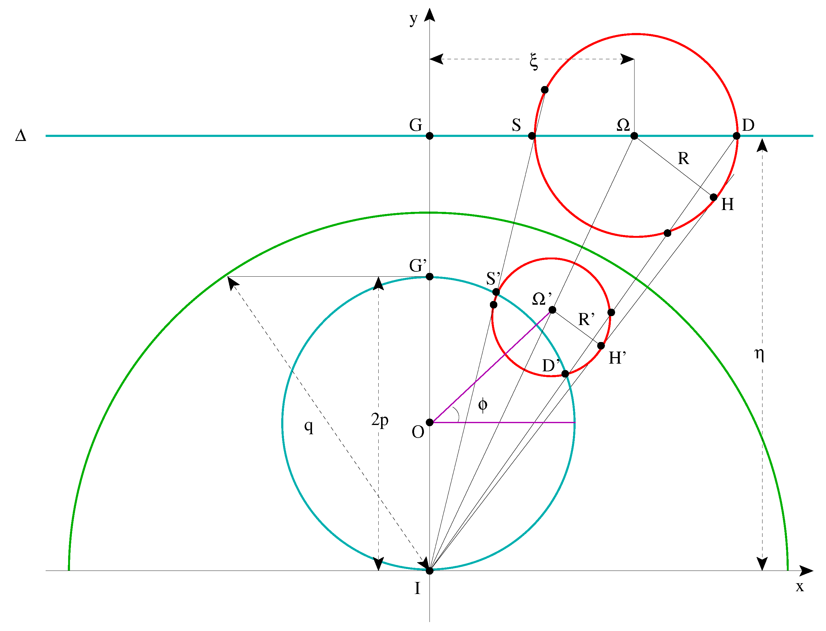
The proposed mapping is a geometric inversion of center I and modulus q (or radius of the inversion circle ). By definition, maps a point to a point , such that and the three points are aligned. Now analytically under this mapping , one has
Clearly is involutive. In Figure 2, we observe the following.
- Line is mapped to circle of center located on the axis and with radius .
- Scanning circle is mapped to apparent scanning circle with center and radius to be determined.
- However, as is orthogonal to , the transformed circle is orthogonal to , this is due to the conformal property of geometric inversion. If intersects at two points S and D, intersects at corresponding points and .
- Moreover, the half circle above (resp. below) line is mapped to the circular arc of inside (resp. outside) . This is because the -line upper half space is mapped to the interior of the disk bounded by the circle . This can be checked geometrically or analytically.
Proposition 2.
Under geometric inversion , and in Cartesian coordinate system , the delta function on a scanning circle becomes
The vanishing of the argument of this delta function defines the equation of , the apparent scanning circle obtained by geometric inversion with center and radius , given in Cartesian coordinate system by
Proof.
Insert (19) in the circle equation
To simplify the expression of the new Radon transform resulting from the application of geometric inversion, we move to the Cartesian coordinate system centered at O, which is deduced by a simple translation in the direction
Then, one has the following.
Corollary 3.
The delta function of the apparent scanning circle in the Cartesian coordinate system is
where is given by Equation (20).
Proof.
By simple substitution. □
We introduce now a particular rationalizing parameterization of the apparent scanning circle , so that the resulting delta function for circle appears in second canonical form.
Proposition 3.
Under the substitution
where constant, and , the delta function on is now
Thus, in Cartesian coordinate system , the apparent scanning circle has center and radius given by
Then, the delta function on in polar coordinates takes the simple form
where .
Proof.
Substitute (24) into the expressions to be calculated and obtain their expressions in terms of the rationalizing parameters
□
5. The Radon Transform on Circles Resulting from Geometric Inversion of Circles Defining the Radon Transform on Circles Centered on a Fixed Line
We are now in a position to transcribe the original Radon data on scanning circles of Equation (16) into data on apparent scanning circles . However, first we should see how the new integration measure transform itself through geometric inversion, shift of coordinate and finally switch to polar coordinates in coordinate system. Following these successive changes of variables,
- the two-dimensional Lebesgue measure becomes
- Moreover, the original density function becomes
It is understood that q as well as p (or ) are given fixed quantities in .
Thus we have the result
Proposition 4.
The original Radon data of on scanning circle can be expressed now as the Radon data on full apparent scanning circles
for the apparent unknown function
Therefore, we may identify . Recall that , with .
Proof.
Therefore, under geometric inversion , the integral of on scanning circles of variable radius R, but centered on fixed line (), may be represented by the integral of an apparent density on apparent scanning circles orthogonal to the fixed circle . This means that geometric inversion has led to the definition of a new Radon transform, which is defined on circles orthogonal to a fixed circle. This Radon transform has been also considered in the framework of hyperbolic geometry, see for example [15]. As a descendent of the previous Radon transform, it suffers also from an ambiguity this time due to an invariance with respect to geometric inversion , as stated in the next proposition
Proposition 5.
The new apparent Radon problem also has an ambiguity as it depends on the inverse (or anallagmatic) symmetric part of .
Proof.
Under geometric inversion , defined by inversion circle , the delta function on apparent scanning circles transforms as
which incidently shows that the scanning circle is globally invariant under this geometric inversion. Then, going over the integration variable , Equation (31) becomes
This shows that depends in fact actually on the inversion (or anallagmatic) even part of or
□
Thus geometric inversion converts the Radon transform on scanning circles centered on line Δ with its Δ-line reflection ambiguity into the Radon transform on apparent scanning circles with its circle anallagmatic ambiguity, where
Therefore, it is natural to identify the mutual correspondence of “partial” Radon transforms.
Theorem 1.
Proof.
The -range is , with and . Moreover, the -ranges are bounded as and .
Do these two “induced” Radon transforms have a physical interpretation? Yes, in the framework of Compton Scatter Tomography (CST), as we shall see in the next section.
6. Concept of Compton Scatter Tomography (CST) and a Special CST Modality
6.1. Overview on SAR, CT, and CST Imaging Processes
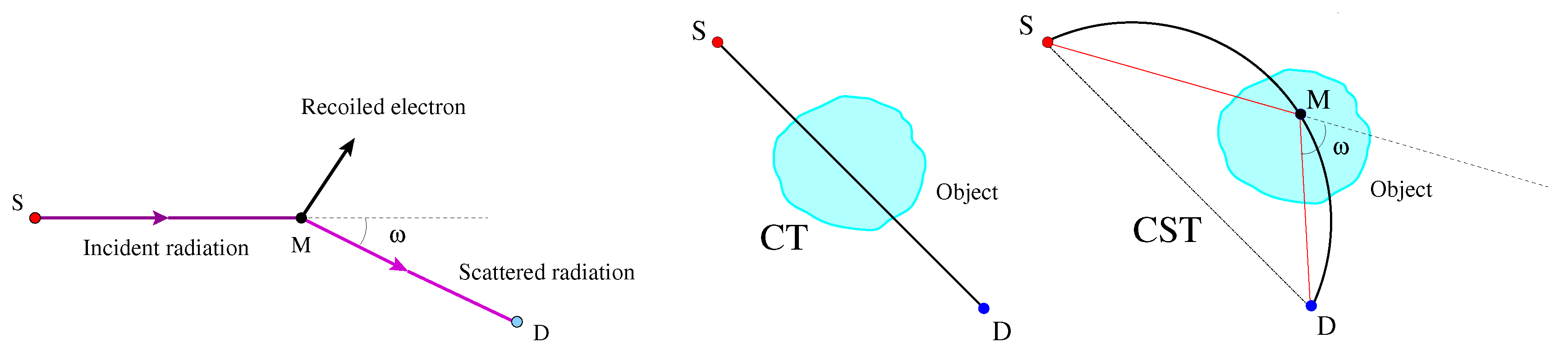
If SAR imaging relies on the law of radiation reflection on material surfaces, Computed Tomography (CT) is based on the law of radiation absorption in matter (Beer’s law). A third imaging possibility which has emerged at the end of last century is the so-called Compton Scatter Tomography (CST). It exploits the law of high-energy radiation scattering on electric charge in matter, which is called the Compton effect. Each of these imaging processes reconstructs a physical density of matter: matter reflectivity density for SAR imaging, matter attenuation density for CT imaging and matter electric charge density for CST imaging. Basically, measurements of detected radiation intensities represent integrals of physical densities on circles for SAR imaging, on straight lines for CT imaging and, as we shall see below, on circular arcs for CST imaging.
The left Figure 3 represents a Compton scattering process, in which an electric charge (electron) is scattered by incoming radiation and deviated by a scattering angle . The scattering law is given by the so-called Compton’s formula
which gives the energy of scattered radiation in terms of the scattering angle ( being a constant and the energy of incoming radiation). Therefore, the measured scattered radiation intensity at an energy-resolved detector D for a given radiation source S will be proportional to the integral of the electric charge density of matter along a circular arc ending at S and D subtending an inscribed angle , see right Figure 3. Thus, a new type of Radon transform defined on a definite family of circular arcs is being now introduced by CST imaging, e.g., for a review see [1]. As families of circular arcs in depend on five parameters, there are many subfamilies dependent on two parameters, one of which should be necessarily the Compton scattering angle . Each two parameter family of circular arcs may be related to a possible CST modality.
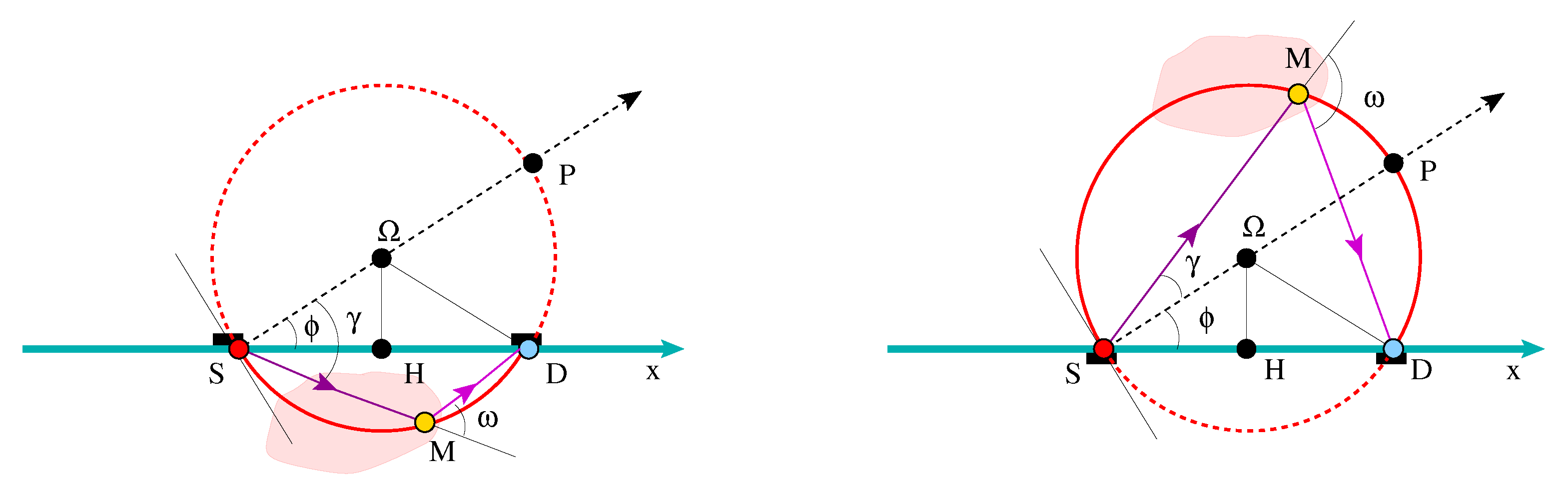
- either a scattered radiation intensity corresponding to a scattering angle , which implies the integration of the electric charge density on some circular arc passing through S and D subtending an angle ,
- or a scattered radiation intensity corresponding to a scattering angle , which corresponds to the integration on a circular arc supplementary to the previous one.
These two supplementary circular arcs belong to a same circle. Therefore, a Radon transform defined on a two parameter family of circles can be naturally decomposed into a sum of two Radon transforms defined on two supplementary two parameter families of circular arcs. As we have seen this splitting is not natural in the case of SAR imaging, but should be introduced by hand.
6.2. A Special CST Modality
This special modality has been found first in [16]. The radiation source S and the scattered radiation detector D move freely on a fixed circle .
- If the detector D is adjusted to record a scattered radiation intensity corresponding to a scattering angle , where is the opening angle , the scanning circular arc is interior to the fixed circle and orthogonal to it. We have here an interior CST reconstruction problem for the electric charge density, see left Figure 5.
- If the detector D is adjusted to record a scattered radiation intensity corresponding to a scattering angle , where , the scanning circular arc is exterior to the fixed circle and orthogonal to it. We have here an exterior CST reconstruction problem for the electric charge density, see right Figure 5.
6.3. Final Reconstruction Formulas
7. Conclusions
In usual contexts of work, symmetry is always a key for reducing the difficulty of a problem to solve. Here, we have given an example to the contrary. The interest of this presentation is to provide a concrete example of theoretical solution to the Radon problem defined on circles centered on a fixed line. To achieve this goal, we have physically separated this Radon problem on circles into two Radon problems on semi-circles lying in separate half spaces. Then, we have mapped them to two naturally separated CST problems for which reconstruction solutions have been established. In the future, it may be interesting to explore the power of geometric inversion (geometric inversion has been used before by [17,18]) or more generally geometric transformations in to seek reconstruction (or inverse)of many Radon transforms in integral geometry.
Funding
This research received no external funding.
Conflicts of Interest
The author declares no conflict of interest.
References
- Truong, T.T.; Nguyen, M.K. Recent Developments on Compton Scatter Tomography: Theory and Numerical Simulations. In Numerical Simulation—From Theory to Industry; Andriychuk, M., Ed.; InTech: Rijeka, Croatia, 2012; Chapter 6; pp. 101–128. [Google Scholar]
- Norton, S.J. Reconstruction of a reflectivity field from line integrals over circular paths. J. Acoust. Soc. Am. 1980, 67, 853–863. [Google Scholar] [CrossRef]
- Haltmeier, M.; Scherzer, O.; Burgholzer, P.; Nuster, R.; Paltauf, G. Thermoacoustic tomography and the circular Radon transform: Exact inversion formula. Math. Model. Methods Appl. Sci. 2007, 17, 635–655. [Google Scholar] [CrossRef]
- Hellsten, H.; Andersson, L.-E. An inverse method for the processing of synthetic aperture radar data. Inverse Probl. 1987, 3, 111–124. [Google Scholar] [CrossRef] [Green Version]
- Fawcett, J. Inversion of n-dimensional spherical averages. SIAM J. Appl. Math. 1985, 45, 336–341. [Google Scholar] [CrossRef]
- Andersson, L.-E. On the determination of a function from spherical averages. SIAM J. Math. Anal. 1988, 19, 214–232. [Google Scholar] [CrossRef]
- Sysoev, S.E. Unique recovery of a function integrable in a strip from its integrals over circles centred on a fixed line. Russ. Math. Surv. 1997, 52, 846–847. [Google Scholar] [CrossRef]
- Rothaus, O.S. Analytic inversion in SAR. Proc. Natl. Acad. Sci. USA 1994, 91, 7032–7035. [Google Scholar] [CrossRef] [PubMed] [Green Version]
- Lindberg, M. Radar Image Processing with Radon Transform; European Consortium for Mathematics in Industry (ECMI). Programme in Applied Mathematics. Technical Report No 5, ISSN 0347-2809; Chalmers Tekniska Högskola/Göteborgs Universitet: Göteborgs, Sweden, 1997; 43p. [Google Scholar]
- Palamodov, V.P. Reconstruction from limited data of arc means. J. Fourier Anal. Appl. 2000, 6, 25–42. [Google Scholar] [CrossRef]
- Redding, N.J.; Newsam, G.N. Inverting the Circular Radon Transform; DSTO Research Report DSTO-RR-0211; Department of Science and Technology Organisation, Electronics and Surveillance Research Laboratory: Edinburgh, Australia, August 2001; 43p. [Google Scholar]
- Redding, N.J.; Payne, T.M. Inverting the Radon transform for 3D-SAR image formation. In Proceedings of the IEEE International Conference on Radar, Adelaide, Australia, 3–5 September 2003; pp. 466–471. [Google Scholar]
- Redding, N.J. SAR image formation via inversion of Radon transform. In Proceedings of the IEEE Intarnational Conference on Image Processing (ICIP), Singapore, 24–27 October 2004; pp. 13–16. [Google Scholar]
- Kettler, D.; Gray, D.; Redding, N.J. The point spread function for UWB SAR imaging using the inversion of the circular Radon transform. In Proceedings of the ENSAR Conference, Dresden, Germany, 4–8 September 2006; pp. 175–178. [Google Scholar]
- Kurusa, A. The Radon transform on hyperbolic space. Geom. Dedicata 1991, 40, 325–339. [Google Scholar] [CrossRef] [Green Version]
- Truong, T.T.; Nguyen, M.K. Radon transforms on generalized Cormack’s curves and a new Compton scatter tomography modality. Inverse Probl. 2011, 27, 125001. [Google Scholar] [CrossRef]
- Quinto, E.T. Singular value decomposition and inversion methods for the exterior Radon transform and a spherical transform. J. Math. Anal. Appl. 1983, 95, 437–448. [Google Scholar] [CrossRef] [Green Version]
- Yagle, A.E. Inversion of spherical means using geometric inversion and Radon transforms. Inverse Probl. 1992, 8, 949–964. [Google Scholar] [CrossRef]
Figure 1.
(a) Left image: Schematic view of Synthetic Antenna Radar (SAR) imaging as Radon transform on circles centered on a fixed line. (b) Right image: Separate (left and right of fixed line) SAR data acquisition.
Figure 1.
(a) Left image: Schematic view of Synthetic Antenna Radar (SAR) imaging as Radon transform on circles centered on a fixed line. (b) Right image: Separate (left and right of fixed line) SAR data acquisition.

Figure 2.
Inversion of scanning circles orthogonal to line into apparent scanning circles orthogonal to the fixed circle .
Figure 2.
Inversion of scanning circles orthogonal to line into apparent scanning circles orthogonal to the fixed circle .

Figure 3.
Left: Compton Effect; Right: Computed Tomography (CT) and Compton Scatter Tomography (CST).
Figure 3.
Left: Compton Effect; Right: Computed Tomography (CT) and Compton Scatter Tomography (CST).

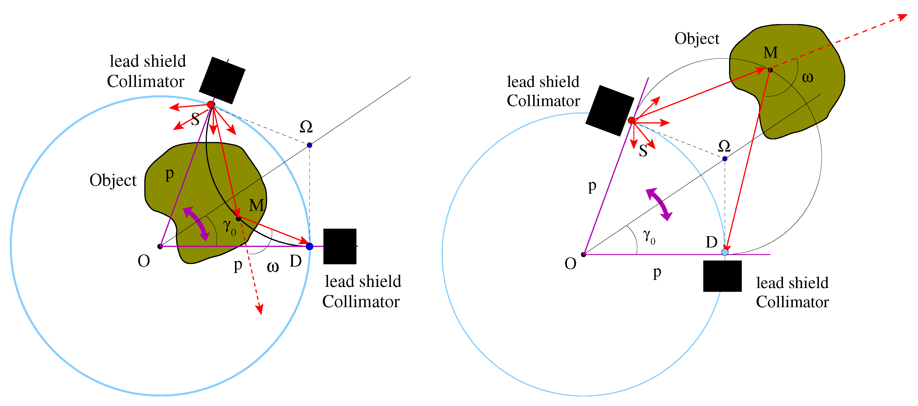
Figure 4.
CST working principle: gamma rays are isotropically emitted by source S, scattered at site M under scattering angle and registered at D. Left image corresponds to , whereas right image corresponds to . For given scattered energy , the locus of M is respectively the lower and the upper circular arc.

Figure 5.
Left: CST Disk internal scanning; Right: CST Disk external scanning.

© 2020 by the author. Licensee MDPI, Basel, Switzerland. This article is an open access article distributed under the terms and conditions of the Creative Commons Attribution (CC BY) license (http://creativecommons.org/licenses/by/4.0/).
Share and Cite
MDPI and ACS Style
Truong, T.T. Function Reconstruction from Reflection Symmetric Radon Data. Symmetry 2020, 12, 956. https://doi.org/10.3390/sym12060956
AMA Style
Truong TT. Function Reconstruction from Reflection Symmetric Radon Data. Symmetry. 2020; 12(6):956. https://doi.org/10.3390/sym12060956
Chicago/Turabian StyleTruong, Trong Tuong. 2020. "Function Reconstruction from Reflection Symmetric Radon Data" Symmetry 12, no. 6: 956. https://doi.org/10.3390/sym12060956
Note that from the first issue of 2016, this journal uses article numbers instead of page numbers. See further details here.