See-Through Near-Eye Display with Built-in Prescription and Two-Dimensional Exit Pupil Expansion

Featured Application

The proposed see-through near-eye display is applicable for the augmented/mixed reality devices, e.g., smart glasses or headsets etc. In addition to being a wearable computing device, it can be used as a pair of everyday eyeglasses with a built-in prescription.

Abstract

We propose a see-through near-eye display featuring an exit pupil expander (EPE), which is composed of two multiplexed slanted gratings. Via a two-dimensional expansion, the exit pupil (EP) is able to be enlarged up to 10 × 8 mm². Besides, the prescription for correcting the refractive errors can be integrated as well. The design rules are set forth in detail, followed by the results and discussion regarding the efficiency, field of view (FOV), exit pupil, angular resolution (AR), modulation transfer function (MTF), contrast ratio (CR), distortion, and simulated imaging.

1. Introduction

Following in the footsteps of smartphones, smart glasses are highly anticipated as the next mobile computing device. Unlike smartphones, which widely adopt the flat panel displays (FPDs) [1,2,3], smart glasses are equipped with see-through near-eye displays (NEDs) [4,5,6]. The major difference between these two types of display technologies is something called an exit pupil (EP). In FPDs, there is no such thing. In NEDs, an exit pupil defines the boundaries to which the eye can be moved. Unfortunately, for the sake of its compact form factor, almost every optical component of NEDs needs to be miniaturized. This inevitably results in a tiny exit pupil. Even when the form factor is overridden, it will not be easy to achieve a big exit pupil owing to the paradox between the field of view (FOV) and the exit pupil [7]. To enlarge the exit pupil, the most common method is to duplicate a single exit pupil into many through multiple reflections and/or diffractions. Of all the techniques that have been reported [8,9,10,11,12,13,14,15,16], the most successful ones are the cascaded semi-reflectors [8] and slanted gratings [10]. The former is a proprietary technology patented by Lumus. However, the cascaded semi-reflectors are only able to duplicate the exit pupil in one dimension. The latter was originally developed by Nokia and later commercialized by Microsoft’s HoloLens. Though HoloLens pulled off the two-dimensional exit pupil duplication, it requires three layers of waveguides with slanted gratings to realize the full color [15]. Another gripe about HoloLens is it is not very friendly for those who have to wear the prescription lens for correcting the refractive errors [17]. For wearable devices, bulkiness is always a deal breaker. Towards the said issues, we hereby introduce a see-through NED that integrates the prescription lens with a two-dimensional exit pupil expander (EPE). In what follows, its structure, design rules, and overall performance are to be expounded.

2. Design Rules

2.1. Proposed Structure

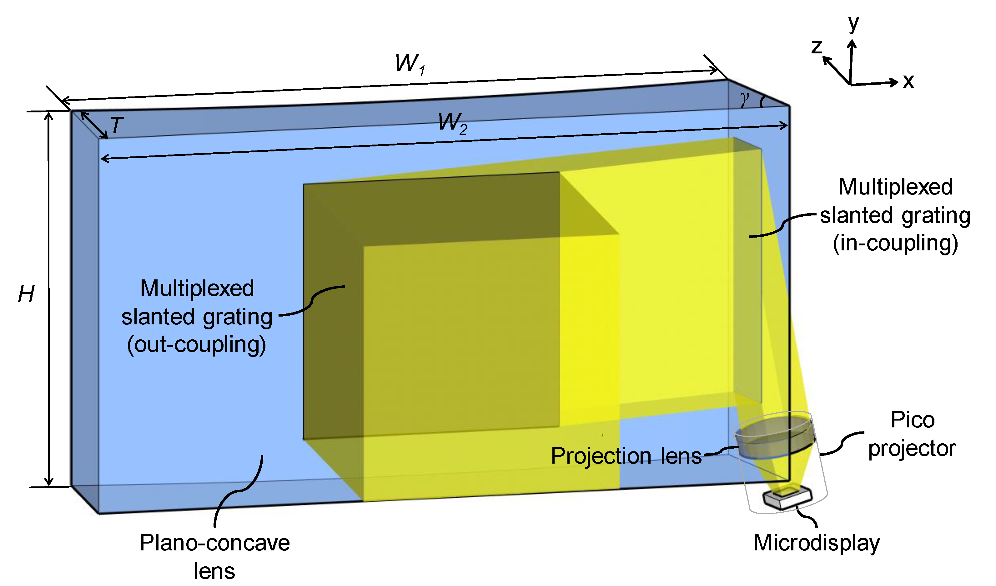
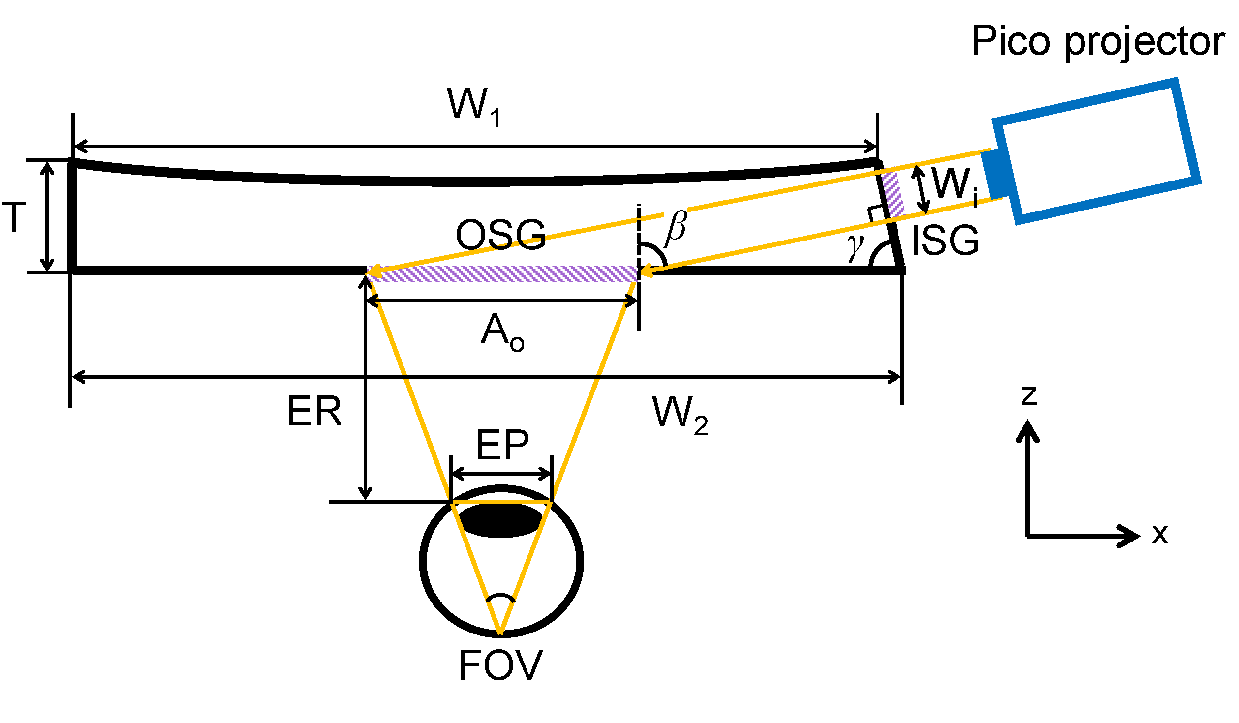
Figure 1 is a schematic of the proposed see-through NED, which consisted of three major components: a pico projector, a plano-concave lens, and two multiplexed slanted gratings. Mounted inside the pico projector was a microdisplay and a projection lens. The front surface (facing forward) of the plano-concave lens was a curved surface, which assumed a concave shape to yield a negative power to compensate the myopia. The right side of plano-concave lens was a bevel, to which the beam of the pico projector was incident. On the bevel, a multiplexed slanted grating was fabricated. This multiplexed slanted grating was able to couple the light from the pico projector into the lens and elongate the beam along the vertical direction. On the back surface (facing the eye) of the plano-concave lens, there was another multiplexed slanted grating that could diffract the light out of the lens and elongate the beam along the horizontal direction. To avoid being confused between these two multiplexed slanted gratings, the former is referred to as the in-coupling slanted grating, or ISG for short, whereas the latter is referred to as the out-coupling slanted grating, or OSG for short. W₁, W₂, H, T, and γ are the front width, back width, height, thickness and bevel angle of plano-concave lens, respectively.

2.2. Plano-Concave Lens

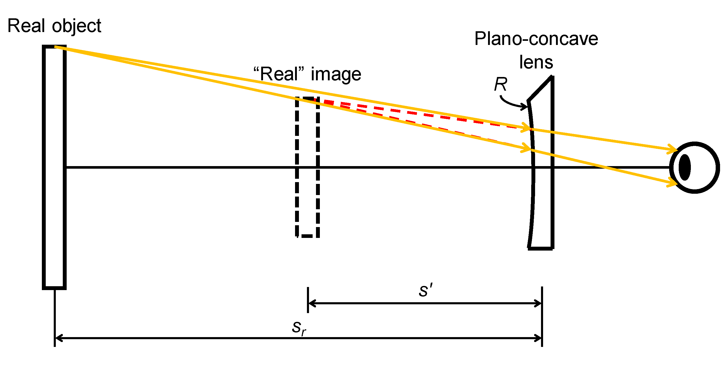
The design of the plano-concave lens was related to the visual acuity, and it plays an important role in imaging the real object, as shown in Figure 2, where R is the radius of curvature of the front surface of lens, s_r the real object distance, and s′ the image distance. For the real image, rays emitted from the real object were diverged by the plano-concave lens so as to offset the over-focusing of the eye. A “real” image―by which we mean that it is the image of a real object, albeit this image is technically virtual―was formed at a closer distance. The object distance s, image distance s′ and diopter or optical power of the lens P shall be correlated via the lens-maker’s equation [18]

$$s^{\prime }=\frac{s_r}{P{s}_r-1}$$

(1)

where

$$P=\frac{n-1}{R}$$

(2)

where n is the refractive index of the lens. Suppose a user has only 3 diopters of myopia, disregarding other types of refractive errors. Then, P = −3 m⁻¹ when s_r = ∞ m and s′ = −0.333 m. It should be mentioned that the “real” image was not observed by the eye. Rather, the eye saw the real object, as the rays derailed by the lens got back on track through the accommodation of the eye [19].

The front width W₁ of the lens rested partly upon the interpupillary distance d_ip, which was on average 64 mm [20]. If the front surface of the lens is center-aligned with the eye, then the front width W₁ of lens is

$$W_1=d_{ip}-d_b$$

(3)

where d_b is the width of the bridge of the smart glasses. Say d_b = 18 mm, W₁ = 46 mm. Further, the front width W₁, back width W₂, thickness T, and bevel angle γ shall be correlated via

$$\frac{T}{W_2-W_1}=tan\gamma$$

(4)

Say γ = 75.52° (as will be discussed later), W₂ = 47.93 mm, and T = 7.47 mm. The height H was a freelance parameter as long as it met the ergonomics. Pursuant to the above design rules, a plano-concave lens can be tentatively designed with the parameters itemized in

Table 1. Parameters for the plano-concave lens.

Object	Parameter	Value
Plano-concave lens	W1	46 mm
	W2	47.93 mm
	H	30 mm
	T	7.47 mm
	γ	75.52°
	Pw	−3 m−1
	n@565 nm	1.5880 1
	R	0.1960 m

¹ Polycarbonate is chosen as the lens material.

.

2.3. Pico Projector

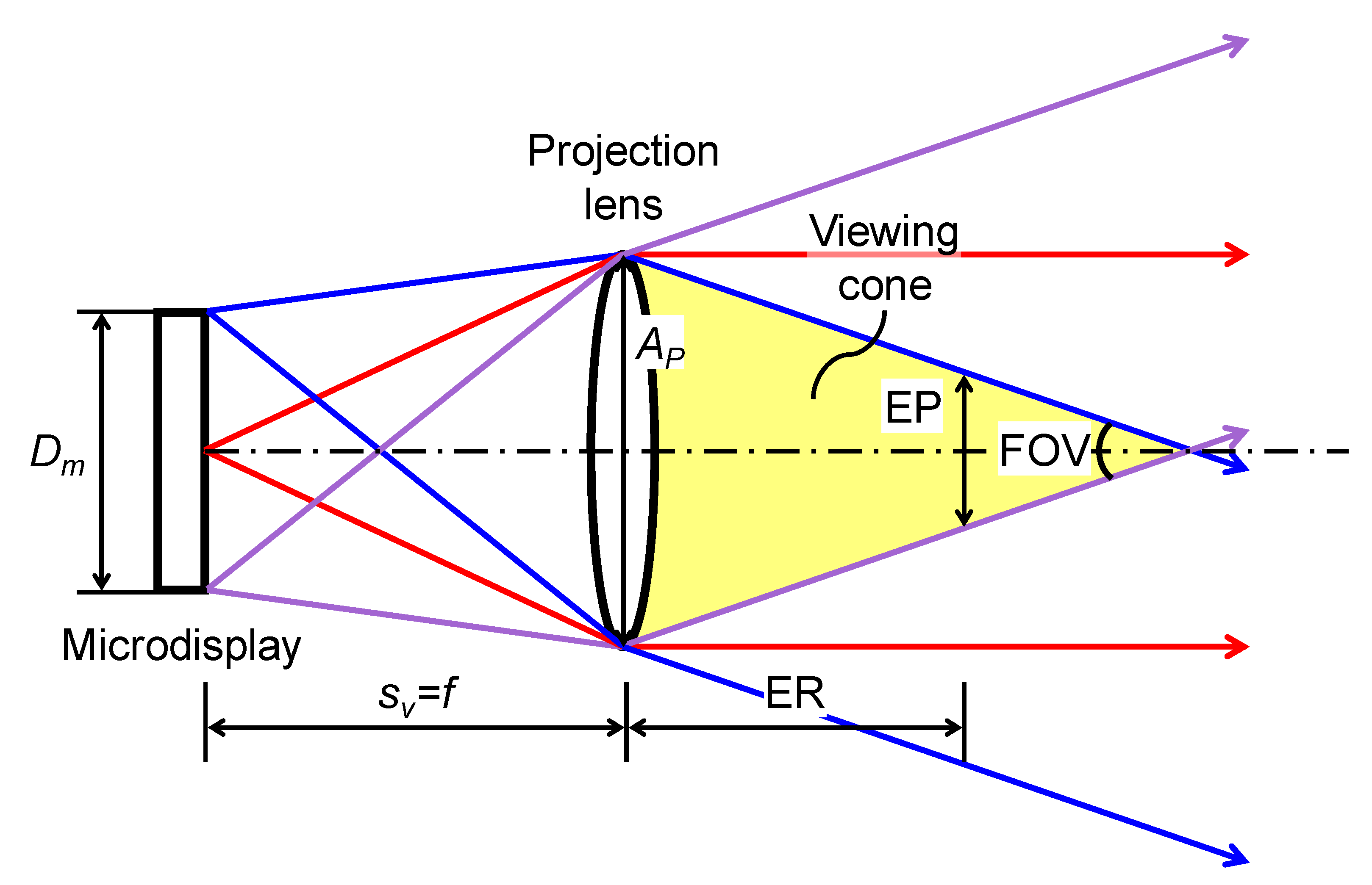
Figure 3 draws the optical path diagram of the pico projector, of which the microdisplay was self-emissive, i.e., organic light-emitting diode panel on silicon [21], and the projection lens was a singlet―namely the simple magnifier. The viewing cone, within which the eye must be placed to see the full image, is highlighted. For the beam to be perfectly collimated, the image distance was set to be infinite by equating the virtual object (microdisplay) distance, s_v, and the focal length, f, of the projection lens. It would be straightforward to write the FOV of the pico projector as

$$FOV=2ta{n}^{-1}\left(\frac{D_m}{2f}\right)$$

(5)

where D_m is the size of the microdisplay. Say D_m = 0.165 inch (4.191 mm) for both horizontal and vertical dimensions and s_v = f = 10 mm, then FOV = 24° (horizontal) × 24° (vertical), i.e., 33° (diagonal). Once the FOV was given, the exit pupil measured at the eye relief (ER)―the distance starting from the last surface of the pico projector to the pupil of eye―could be determined with

$$EP=A_p-2·ER·tan\left(\frac{FOV}{2}\right)$$

(6)

where A_p is the aperture of the projection lens, and also the entrance pupil of our system. If the ER = 12 mm and A_p = 6 mm, then EP = 1 mm, which is unacceptably small. Since there is not much room to further shorten the eye relief―especially for NEDs without a built-in prescription―the simplest way to expand the exit pupil was to scale up the projection lens. That being said, the wearability was compromised due to the added volume and weight.

Table 2. Parameters of the pico projector.

Object	Parameter	Value
Microdisplay	Dm (diagonal)	0.233 inch
	Dm (horizontal/vertical)	0.165 inch
	Resolution	640 × 640
	Pixel size	6.5 µm
	CR	100,000
Projection lens	f	10 mm
	FOV (diagonal)	33°
	FOV (horizontal/vertical)	24°
	Aperture	6 mm
	ER	12 mm
	EP	1 mm

lists the customized specifications necessary for designing the pico projector. Other than the values already mentioned, the resolution of the microdisplay was 640 × 640, the pixel size was 6.5 µm, and the contrast ratio (CR) was 100,000.

2.4. Multiplexed Slanted Grating

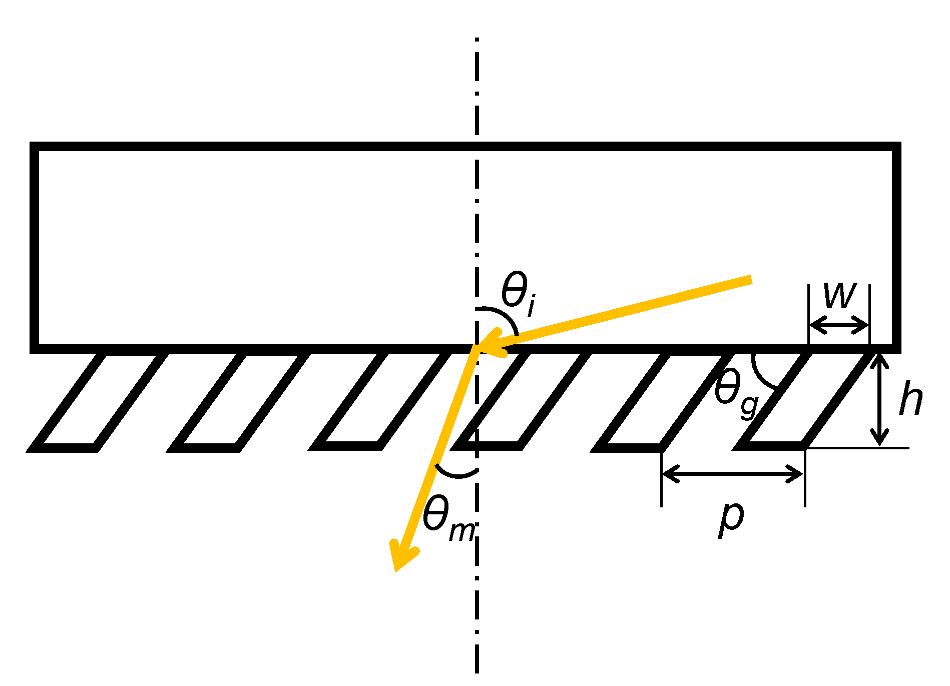
Slanted grating, a type of asymmetric grating, lends itself to folding the optical path of see-through NEDs for the reason that the energy of diffracted light can be concentrated to a certain diffraction order [22]. Its cross-sectional profile is outlined in Figure 4, where p is the grating period, h the grating height, w the grating width, and θ_g the slant angle. To couple light into and out of the lens, both the ISG and OSG were constructed as the transmission gratings, whose allowable diffraction angles shall satisfy [22]

$$p\left(n_{i}sin{\theta }_i-n_{e}sin{\theta }_m\right)=m\lambda$$

(7)

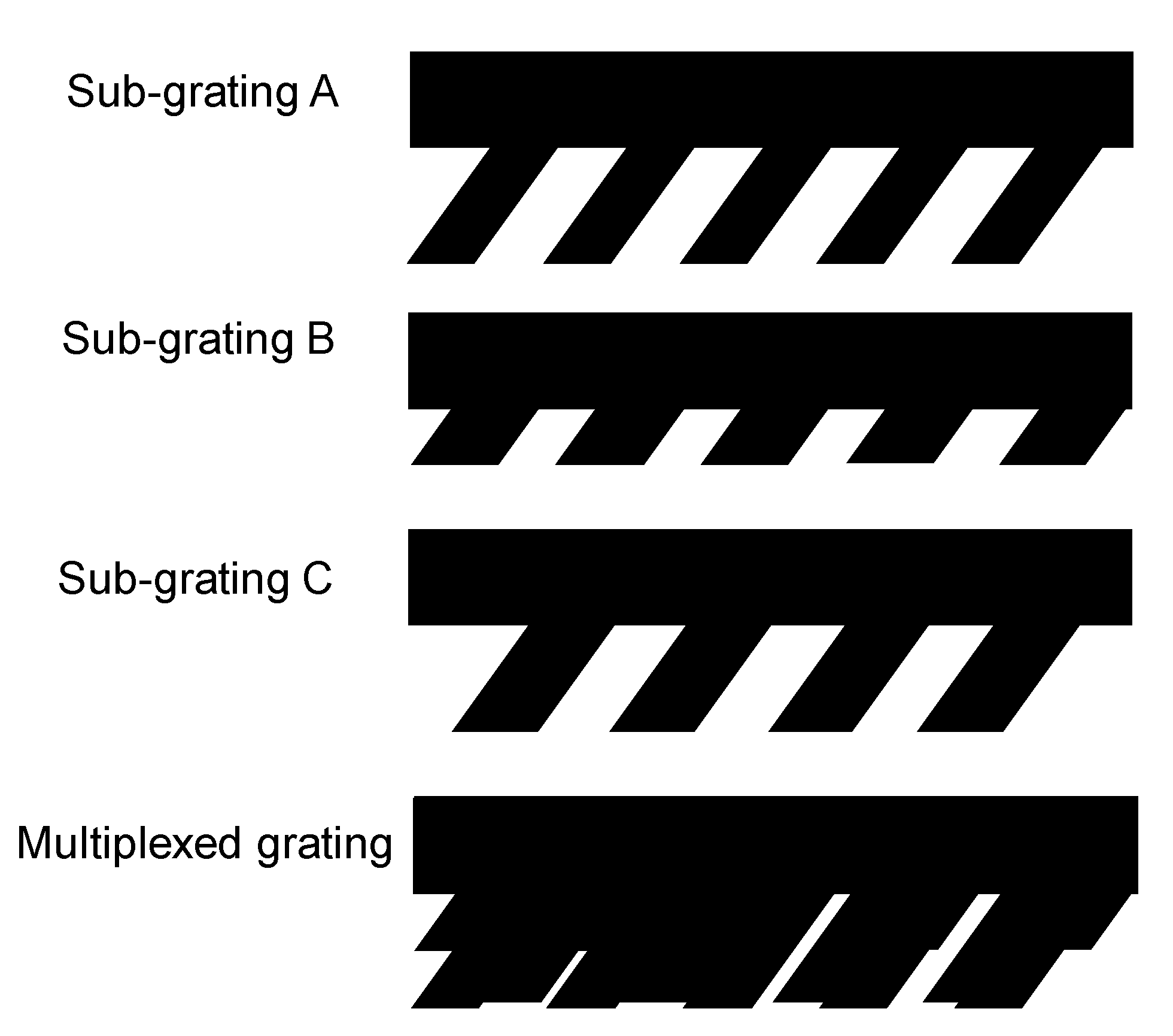
where n_i is the refractive index of the incident medium, n_e the refractive index of the exit medium, θ_i the incident angle (relative to the grating normal), θ_m the diffraction angle of m^th order, m the diffraction order, and λ the wavelength. As Equation (7) indicates, for a single-period slanted grating, both of its spectral and angular bandwidths were intrinsically narrow. To solve this issue, a multiple of waveguides with different gratings can be stacked together for the full color [15]. As an alternative solution, we resorted to the multiplexing of plural gratings on a single layer [23,24]. The multiplexed grating can be decomposed into three sub-gratings of the same slant angle but of different periods, widths and heights, as shown in Figure 5. Each sub-grating was designed for certain wavelength and incident angle. Say the periods of sub-gratings are p_A, p_B, and p_C, respectively, then the collective period P_m of the multiplexed grating shall be the least common multiple of the above three. To minimize the reflection at the interface between the grating and the lens, it was desirable to etch the slanted gratings out of the lens so that there is no mismatch in their refractive indices. Speaking of the fabrication, photolithography, electron-beam lithography, and focused ion beam are among the feasible lithography techniques [25].

2.5. Exit Pupil Expansion

Instead of duplicating the exit pupil into many, our EPE leveraged the oblique intersection of the viewing cone. As shown in Figure 6, the plane of the ISG intersected the viewing cone at angle α, thereby forming an elliptical exit pupil, which had a vertical length A_i that can be written as

$$A_i=A_{p}sin\alpha +\frac{A_{p}cos\alpha }{tan\left(\frac{FOV}{2}+\alpha \right)}$$

(8)

and a horizontal length that is defined by the width W_i of the ISG. Say A_p = 6 mm and α = 14.48°, A_i = 13.25 mm. Let β symbolize the angle of beam incident to the OSG, as shown in Figure 7, where only the axial rays are depicted. The horizontal length of the elliptical exit pupil will be elongated to A_o

$$A_o=\frac{W_i}{cos\beta }$$

(9)

For W_i = 3.8 mm and β = 75.52°, A_o = 15.2 mm. As a result, the ISG is of 3.8 × 13.25 mm² and the OSG of 15.2 × 13.25 mm². In case of misalignment, their actual sizes were supposed to be bigger. If the beam incident to the OSG is perpendicular to the bevel or the ISG, then β is equal to the bevel angle γ, which affects the thickness of the plano-concave lens. Incidentally, for the off-axis rays, problems such as pupil mismatch, vignetting, etc. merit special care.

3. Results and Discussion

3.1. Simulation Settings

The performance of our NED is quantitatively analyzed with Code V (Synopsys) and VirtualLab Fusion (Wyrowski Photonics). The former deals with the modulation transfer function (MTF), distortion, and simulated images. The latter handles the diffraction efficiency (DE) of multiplexed slanted gratings. The design wavelengths include 495, 565, and 655 nm. The real and virtual images are simulated in forward and backward directions, respectively. The parameters of optical surfaces used for both the real and virtual images are summarized in

Table 3. Optical surfaces used in the simulation of the real image.

Surface	Surface Type	Radius (mm)	Thickness (mm)	Refractive Index 1	Semi-Aperture (mm)
real object	sphere	infinity	infinity
1	asphere	−196.0000	7.4700	1.5880	1.5000
2	sphere	infinity	−336.2359		2.6760
real image	sphere	infinity	0		99.7948

¹ Refractive index is left empty when the medium is air.

and

Table 4. Optical surfaces used in the simulation of the virtual image.

Surface	Surface Type	Radius (mm)	Thickness (mm)	Refractive Index 1	Semi-Aperture (mm)
virtual image	sphere	infinity	infinity
1	asphere	4.1494	3.6000	1.7258	3.0000
2	asphere	4.1379	10.0000		2.2399
microdisplay	sphere	infinity	0.0000		3.4613

¹ Refractive index is left empty when the medium is air.

. More detailed parameters for defining aspherical surfaces can be found in

Table 5. Detailed parameters of aspherical surfaces for the real image.

Surface	Y Radius (mm)	Conic Constant (K)	4th Order Coefficient (A)	6th Order Coefficient (B)	8th Order Coefficient (C)
1	−196.0000	0.0000	0.0003	−0.0001	2.7720 × 10−5

and

Table 6. Detailed parameters of aspherical surfaces for the virtual image.

Surface	Y Radius (mm)	Conic Constant (K)	4th Order Coefficient (A)	6th Order Coefficient (B)	8th Order Coefficient (C)	10th Order Coefficient (D)	12th Order Coefficient (E)
1	4.1494	−0.1154	0.0003	5.7069 × 10−7	6.9614 × 10−6	−5.4048 × 10−7	2.1806 × 10−8
2	4.1379	−0.6547	0.0055	0.0003	0.0003	−6.7023 × 10−5	9.9782 × 10−6

.

3.2. Diffraction Efficiency

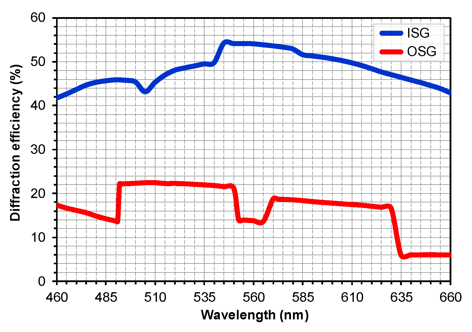
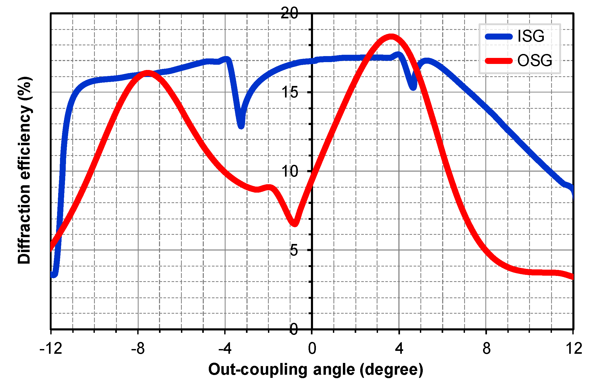
The algorithm for calculating the grating is the Fourier modal method [26]. The simulated annealing method [27] and Nelder–Mead or downhill simplex method [28] are in turn employed for the global and local optimizations. During the optimization, the slant angle, grating height and width are assigned as variables. In order to widen the spectral and angular bandwidths of a single slanted grating, both the ISG and OSG are multiplexed, which are formed through the fusion of plural sub-gratings, as itemized in

Table 7. Optimized parameters of the ISG and OSG.

Object	Sub-Object	Parameter	Value
ISG	Sub-grating A	p	511 nm
		h	1015.80 nm
		θg	29.31°
		w	55.67 nm
	Sub-grating B	p	587 nm
		h	637.79 nm
		θg	29.31°
		w	272.30 nm
	Sub-grating C	p	688 nm
		h	697.85 nm
		θg	29.31°
		w	244.51 nm
	Multiplexed grating	Pm	19.95 μm
OSG	Sub-grating A	p	317 nm
		h	702.98 nm
		θg	42.413°
		w	128.67 nm
	Sub-grating B	p	364 nm
		h	440.53 nm
		θg	42.413°
		w	237.36 nm
	Sub-grating C	p	427 nm
		h	633.81 nm
		θg	42.413°
		w	310.07 nm
	Multiplexed grating	Pm	12.39 μm

. As for the spectral bandwidth, the DEs of all possible diffraction orders combined are calculated with respect to the wavelengths, as shown in Figure 8, where the average DEs of the ISG and OSG over the entire spectrum (460 to 660 nm) are 48.0% and 16.7%, respectively. As for the angular bandwidth, the DEs are calculated with respect to the out-coupling angles, at which the light is coupled out of the lens, the range of which equals the FOV, as shown in Figure 9. It can be seen that the average DEs of the ISG and OSG for the wavelength of 565 nm over the full horizontal/vertical FOV (±12°) are 14.40% and 10.53%, respectively.

3.3. Total Efficiency

Total efficiency, η, which measures the overall light utilization, is defined as the ratio of illuminance at the plane of the microdisplay to that at the plane of the exit pupil. Provided that the absorption, reflection and scattering of both projection and the prescription lenses are neglected, total efficiency η could be roughly estimated with

$$\eta =\frac{1}{{f\#}^2}D{E}_{i}D{E}_o$$

(10)

where

$$f\#=\frac{f}{A_p}$$

(11)

where f# stands for the f-number of the projection lens, DE_i the average DE of the ISG, DE_o the average DE of the OSG, and A_p the diameter of the entrance pupil. For our projection lens, f = 10 mm, A_p = 6 mm, thus f# = 1.67. For the entire FOV at the wavelength of 565 nm, DE_i = 14.4% and DE_o = 10.5%, thus η = 0.55%.

3.4. Field of View

The FOV of the real image, FOV_r, describes the angular extent of the curved front surface of the plano-concave lens, which is given by

$$FO{V}_r=2·ta{n}^{-1}\left(\frac{\sqrt{w_1^2+H^2}}{2ER}\right)$$

(12)

It can be seen that FOV_r is limited by the size of the plano-concave lens. As W₁ = 46 mm, H = 30 mm (see Table 1), and ER = 12 mm, FOV_r = 133° (125° × 103°). The FOV of the virtual image, FOV_v, hinges on both the pico projector and gratings. As the out-coupling angles of the ISG and OSG span over the input FOV of the pico projector, the output FOV_v is therefore conserved as 33° (24° × 24°), which is comparable to HoloLens 1′s FOV [15].

3.5. Exit Pupil

Without the exit pupil expansion, the original exit pupil at the eye relief of 12 mm is 1 × 1 mm². Revisiting Figure 7 and Equation (6), the final exit pupil becomes

$$EP=A_{o/i}-2·ER·tan\left(\frac{FOV}{2}\right)$$

(13)

For ER = 12 mm, A_o/i = 15.2 or 13.25 mm, and FOV = 24° × 24°, EP = 10 × 8 mm². It shall be noted that although both the expanded and duplicated exit pupils can be calculated in the same way, the expanded exit pupil without gaps is undisputedly more solid than the duplicated exit pupils with gaps in between [8,9,10,11,12,13,14,15,16].

3.6. Angular Resolution

For the virtual image, angular resolution (AR) is defined as the average angular subtense of a single pixel. It can be calculated by dividing the FOV―measured in arcminutes (′)―by the number of pixels N along the diagonal, which is stated as [29]

$$AR=\frac{60·FO{V}_v}{N}=\frac{60·FO{V}_v}{\sqrt{N_h^2+N_v^2}}$$

(14)

where N_h and N_v are the number of pixels along the horizontal and vertical directions, respectively. For FOV_v = 33°, N_h = 640, and N_v = 640, AR = 2.19′.

3.7. Modulation Transfer Function

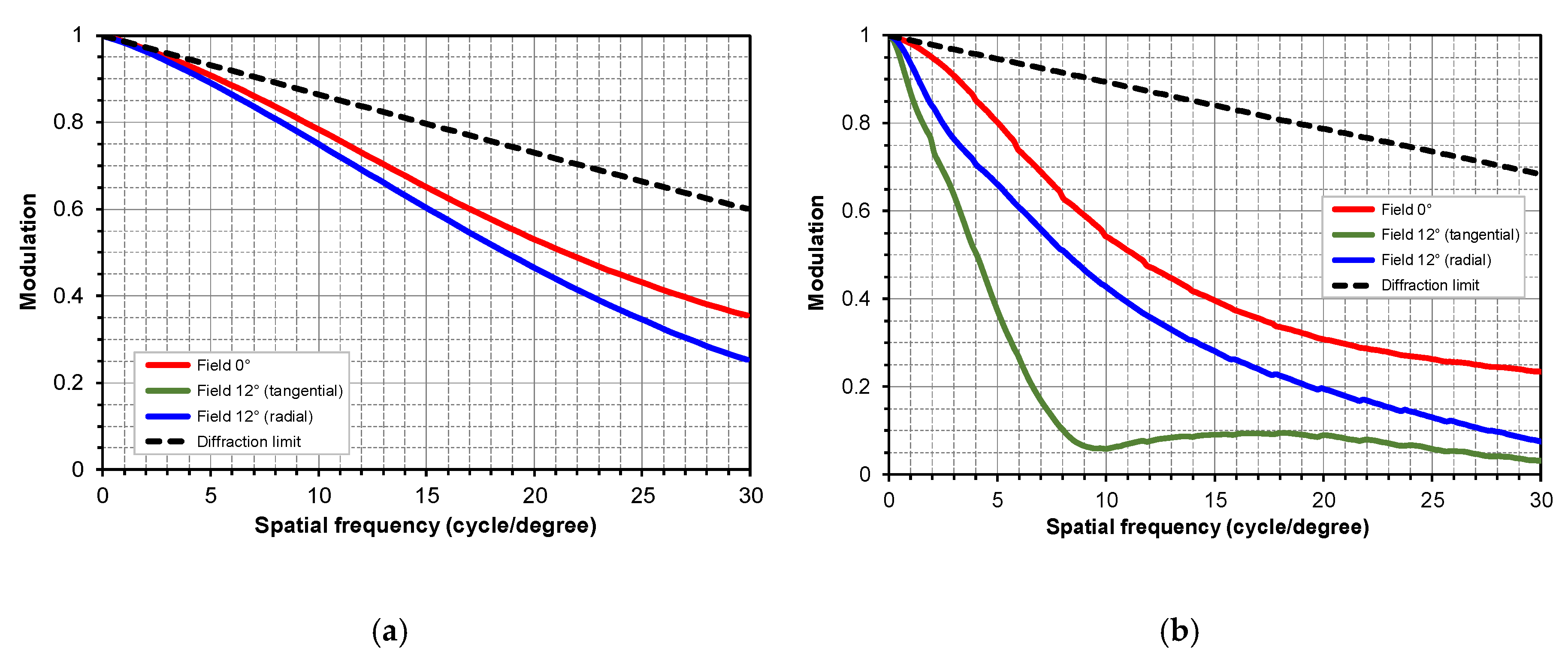
As shown in Figure 10, the MTFs are calculated as a function of spatial frequency in cycle/degree for the fields of 0° and 12° (tangential and radial). At 30 cycle/degree, the MTFs for all fields of the real and virtual images are above 0.252 and 0.032, respectively. The reason why the MTFs at 30 cycle/degree are selected as a benchmark is linked to the visual acuity [30]. A normal visual acuity of 1.0―stated as a decimal number―means that the eye is able to read an optotype at a spatial frequency of 30 cycle/degree.

3.8. Contrast Ratio

CR―the ratio of maximum intensity to minimum intensity―can be deduced as [31]

$$C{R}_{r/v}=\frac{C{R}_0+1+\left(C{R}_0-1\right)·MTF}{C{R}_0+1-\left(C{R}_0-1\right)·MTF}$$

(15)

where CR_o is the CR of the real/virtual object. As the horizontal/vertical resolution is 640 and the FOV = 24°, the corresponding spatial frequency shall be 13.33 cycle/degree. According to Figure 10, at the field of 0° for the real image, CR_r = 5 (CR_o = ∞ and MTF = 0.69), while for the virtual image, CR_v = 3 (CR_o = 100,000 and MTF = 0.44).

3.9. Distortion

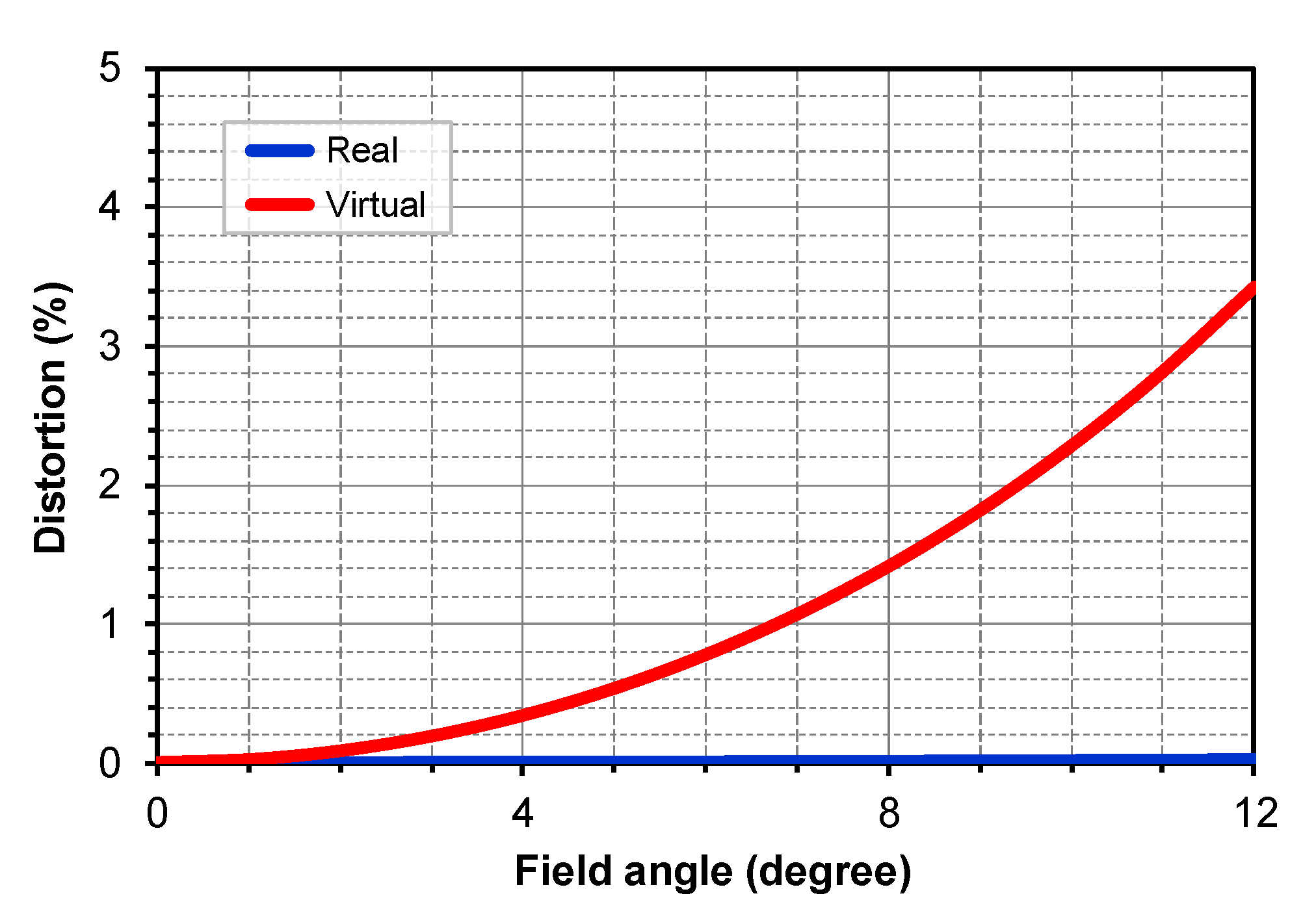
Distortion―the displacement of image height or ray location―is plotted in Figure 11, from which it can be seen that the distortions are 0.02% and 3.4% for the real and virtual images, respectively.

3.10. Simulated Imaging

Figure 12 shows the original image alongside the real and virtual images. Compared to the original one, the real image is virtually lossless, while the virtual image has a mild pincushion distortion and slightly decreased brightness.

4. Conclusions

A see-through NED with a built-in prescription and two-dimensional EPE and design rules thereof have been proposed. Via a two-dimensional expansion, its exit pupil is enlarged up to 10 × 8 mm². As opposed to the conventional EPEs, in which the exit pupil is duplicated or cloned into many, our solution leverages the oblique intersection of the viewing cone. More importantly, full color can be realized by the multiplexed gratings on a single layer. Other than the EPE, another benefit is the integration of prescriptions for a better user experience. Based on the simulation, its overall performance, including the efficiency, FOV, AR, MTF, CR, distortion, and simulated imaging have been investigated. For the real image, the FOV is 133° (diagonal), MTF is above 0.252 at 30 cycle/degree, CR is 5, and distortion is 0.02%. For the virtual image, the total efficiency is 0.55%, FOV is 33° (diagonal), AR is 2.19′, MTF is above 0.032 at 30 cycle/degree, CR is 3, and distortion is 3.4%. Merits aside, low efficiency, pupil mismatch, vignetting, etc. are identified as the remaining issues and will be dealt with in our future work.

References

- Chen, C.; Li, H.; Zhang, Y.; Moon, C.; Kim, W.Y.; Jhun, C.G. Thin-film encapsulation for top-emitting organic light-emitting diode with inverted structure. Chin. Opt. Lett. 2014, 12, 022301. [Google Scholar] [CrossRef]
- Chen, C.P.; Li, Y.; Su, Y.; He, G.; Lu, J.; Qian, L. Transmissive interferometric display with single-layer Fabry-Pérot filter. J. Disp. Technol. 2015, 11, 715–719. [Google Scholar] [CrossRef]
- Chen, C.P.; Wu, Y.; Zhou, L.; Wang, K.; Zhang, Z.; Jhun, C.G. Crosstalk-free dual-view liquid crystal display using patterned E-type polarizer. Appl. Opt. 2017, 56, 380–384. [Google Scholar] [CrossRef] [PubMed] [Green Version]
- Hu, X.; Hua, H. High-resolution optical see-through multi-focal-plane head-mounted display using freeform optics. Opt. Express 2014, 22, 13896–13903. [Google Scholar] [CrossRef] [PubMed]
- Zhou, L.; Chen, C.P.; Wu, Y.; Zhang, Z.; Wang, K.; Yu, B.; Li, Y. See-through near-eye displays enabling vision correction. Opt. Express 2017, 25, 2130–2142. [Google Scholar] [CrossRef] [PubMed]
- Wu, Y.; Chen, C.P.; Zhou, L.; Li, Y.; Yu, B.; Jin, H. Design of see-through near-eye display for presbyopia. Opt. Express 2017, 25, 8937–8949. [Google Scholar] [CrossRef] [PubMed]
- Mi, L.; Chen, C.P.; Lu, Y.; Zhang, W.; Chen, J.; Maitlo, N. Design of lensless retinal scanning display with diffractive optical element. Opt. Express 2019, 27, 20493–20507. [Google Scholar] [CrossRef] [PubMed]
- Amitai, Y. Extremely compact high-performance HMDs based on substrate-guided optical element. In Proceedings of the SID International Symposium, Seattle, WA, USA, 23–28 May 2004; pp. 310–313. [Google Scholar]
- Amitai, Y. A two-dimensional aperture expander for ultra-compact, high-performance head-worn displays. In Proceedings of the SID International Symposium, Boston, MA, USA, 22–27 May 2005; pp. 360–363. [Google Scholar]
- Levola, T. Diffractive optics for virtual reality displays. J. Soc. Inf. Disp. 2006, 14, 467–475. [Google Scholar] [CrossRef]
- Levola, T.; Aaltonen, V. Near-to-eye display with diffractive exit pupil expander having chevron design. J. Soc. Inf. Disp. 2008, 16, 857–862. [Google Scholar] [CrossRef]
- Ayras, P.; Saarikko, P.; Levola, T. Exit pupil expander with a large field of view based on diffractive optics. J. Soc. Inf. Disp. 2009, 17, 659–664. [Google Scholar] [CrossRef]
- Vallius, T.; Tervo, J. Waveguides with Extended Field of View. U.S. Patent 9,791,703 B1, 13 April 2016. [Google Scholar]
- Liu, Z.; Pang, Y.; Pan, C.; Huang, Z. Design of a uniform-illumination binocular lens display with diffraction gratings and freeform optics. Opt. Express 2017, 25, 30720–30731. [Google Scholar] [CrossRef] [PubMed]
- Kress, B.C.; Cummings, W.J. Towards the ultimate mixed reality experience: HoloLens display architecture choices. In Proceedings of the SID Display Week 2017, Los Angeles, CA, USA, 21–26 May 2017; pp. 127–131. [Google Scholar]
- Grey, D.; Talukdar, S. Exit Pupil Expanding Diffractive Optical Waveguiding Device. U.S. Patent 10,359,635 B2, 14 August 2018. [Google Scholar]
- Wu, Y.; Chen, C.P.; Zhou, L.; Li, Y.; Yu, B.; Jin, H. Near-eye display for vision correction with large FOV. In Proceedings of the SID Display Week 2017, Los Angeles, CA, USA, 21–26 May 2017; pp. 767–770. [Google Scholar]
- Pedrotti, F.L.; Pedrotti, L.M.; Pedrotti, L.S. Introduction to Optics, 3rd ed.; Springer: London, UK, 2006. [Google Scholar]
- Wikipedia. Accommodation (Eye). Available online: https://en.wikipedia.org/wiki/Accommodation_(eye) (accessed on 12 May 2020).
- Gross, H.; Blechinger, F.; Achtner, B. Handbook of Optical Systems Volume 4: Survey of Optical Instruments, 1st ed.; Wiley: Hoboken, NJ, USA, 2008. [Google Scholar]
- Armitage, D.; Underwood, I.; Wu, S.-T. Introduction to Microdisplays, 1st ed.; Wiley: Hoboken, NJ, USA, 2006. [Google Scholar]
- Loewen, E.G.; Popov, E. Diffraction Gratings and Applications, 1st ed.; Marcel Dekker: New York, NY, USA, 1997. [Google Scholar]
- Xiao, J.; Liu, J.; Han, J.; Wang, Y. Design of achromatic surface microstructure for near-eye display with diffractive lens. Opt. Commun. 2019, 452, 411–416. [Google Scholar] [CrossRef] [Green Version]
- He, Z.; Chen, C.P.; Gao, H.; Shi, Q.; Liu, S.; Li, X.; Xiong, Y.; Lu, J.; He, G.; Su, Y. Dynamics of peristrophic multiplexing in holographic polymer-dispersed liquid crystal. Liq. Cryst. 2014, 41, 673–684. [Google Scholar] [CrossRef]
- Cui, Z. Nanofabrication: Principles, Capabilities and Limits, 2nd ed.; Springer: Cham, Switzerland, 2017. [Google Scholar]
- Li, L. New formulation of the Fourier modal method for crossed surface-relief gratings. J. Opt. Soc. Am. A 1997, 14, 2758–2767. [Google Scholar] [CrossRef]
- Wikipedia. Simulated Annealing. Available online: https://en.wikipedia.org/wiki/Simulated_annealing (accessed on 12 May 2020).
- Wikipedia. Nelder–Mead Method. Available online: https://en.wikipedia.org/wiki/Nelder–Mead_method (accessed on 12 May 2020).
- Wu, Y.; Chen, C.P.; Mi, L.; Zhang, W.; Zhao, J.; Lu, Y.; Guo, W.; Yu, B.; Li, Y.; Maitlo, N. Design of retinal-projection-based near-eye display with contact lens. Opt. Express 2018, 26, 11553–11567. [Google Scholar] [CrossRef] [PubMed]
- Chen, J.; Mi, L.; Chen, C.P.; Liu, H.; Jiang, J.; Zhang, W. Design of foveated contact lens display for augmented reality. Opt. Express 2019, 27, 38204–38219. [Google Scholar] [CrossRef] [PubMed]
- Chen, C.P.; Zhou, L.; Ge, J.; Wu, Y.; Mi, L.; Wu, Y.; Yu, B.; Li, Y. Design of retinal projection displays enabling vision correction. Opt. Express 2017, 25, 28223–28235. [Google Scholar] [CrossRef]
Figure 1.
Schematic of the proposed see-through near-eye display (NED). W1, W2, H, T, and γ are the front width, back width, height, thickness and bevel angle of plano-concave lens, respectively.
Figure 2.
Optical path diagram for imaging the real object. R is the radius of curvature of the front surface of lens, sr the real object distance, and s′ the image distance.
Figure 3.
Optical path diagram of the pico projector. Dm is the size of the microdisplay, sv the virtual object distance, f the focal length of the projection lens, Ap the aperture of the projection lens, FOV the field of view, ER the eye relief, and EP the exit pupil.
Figure 4.
Cross-sectional profile of slanted grating. p is the grating period, h the grating height, w the grating width, θg the slant angle, θi the incident angle (relative to the grating normal), and θm the diffraction angle of mth order.
Figure 5.
Decomposition of multiplexed grating into three sub-gratings. Say the periods of sub-gratings are pA, pB, and pC, respectively, then the collective period Pm of the multiplexed grating shall be the least common multiple of the above three.
Figure 6.
Illustration of the vertical expansion of the exit pupil by the in-coupling slanted grating (ISG). α is the angle between the optical axis of viewing cone and the plane of the ISG, Ap the aperture of the projection lens, Ai the vertical length of intersected exit pupil.
Figure 7.
Illustration of the horizontal expansion of the exit pupil by the out-coupling slanted grating (OSG). β is the angle of beam incident to OSG, γ the bevel angle, Wi the width of the ISG, Ao the horizontal length of elongated exit pupil.
Figure 8.
Diffraction efficiencies (DEs) of all possible diffraction orders combined of the ISG and OSG calculated with respect to the wavelength. The average DEs of the ISG and OSG over the entire spectrum (460 to 660 nm) are 48.0% and 16.7%, respectively.
Figure 9.
Diffraction efficiencies of the ISG and OSG calculated with respect to the out-coupling angle for the wavelength of 565 nm. The average DEs of the ISG and OSG over the full horizontal/vertical FOV (±12°) are 14.40% and 10.53%, respectively.
Figure 10.
Calculated MTFs of (a) real and (b) virtual images. At the spatial frequency of 30 cycle/degree, MTFs for all fields of the real and virtual images are above 0.252 and 0.032, respectively.
Figure 11.
Calculated distortion with respect to the field angle. It can be seen that the distortions are 0.02% and 3.4% for the real and virtual images, respectively.
Figure 12.
(a) Original (photographer: C. P. Chen, location: Peterhof Grand Palace, St. Petersburg, Russia), (b) real, and (c) virtual images. Compared to the original one, the real image is virtually lossless, while the virtual image has a mild pincushion distortion and slightly decreased brightness.