Numerical and Experimental Study of Turbulent Mixing Characteristics in a T-Junction System


1
School of Water Conservancy Engineering, Zhengzhou University, Zhengzhou 450001, China
2
National Local Joint Engineering Laboratory of Major Infrastructure Testing and Rehabilitation Technology, Zhengzhou 450001, China
3
Collaborative Innovation Center of Water Conservancy and Transportation Infrastructure Safety, Zhengzhou 450001, China
*
Authors to whom correspondence should be addressed.
Appl. Sci. 2020, 10(11), 3899; https://doi.org/10.3390/app10113899
Submission received: 25 April 2020
/
Revised: 29 May 2020
/
Accepted: 3 June 2020
/
Published: 4 June 2020
Abstract
:The mixing, migration, and degradation of pollutants in sewers are the main causes for pipeline corrosion and the increased pollution scope. The clarification of the turbulent mixing characteristics in pipelines is critical for finding the source of pollution in a timely fashion and inspecting pipelines’ damaged locations. In this paper, numerical simulations and experiments were conducted to investigate the turbulent mixing characteristics in pipelines by studying a T-junction system, of which four variables (main pipe diameter φ, cross-flow flux Q, mixing ratio δ, the incident angle of T-junctions θ) were considered. The coefficient of variation (COV) of the salt solution was selected as the evaluation index and effective mixing length (LEML) was defined for quantitative analysis. The numerical results were found to be in good agreement with the experimental results. The results reveal that the values of LEML rise as Q or φ increase and decrease with the increase of δ, where the influence of φ is much greater than Q and δ, and there is no obvious regularity between LEML and θ. By dimensional analysis and multivariate nonlinear regression analysis, a dimensionless relationship equation in harmony with the dimensional analysis was fitted, and a simplified equation with the average error of 4.01% was obtained on the basis of correlation analysis.
1. Introduction
Sewers as indispensable infrastructures in urban development, are located in all corners of the city, which undertake the sewage conveyance, water pollution control, flood control, storm drainage, and other significant functions. After the heavy rainfall flood, the sewers may be full at one place due to the large increase of flow. When the sewers break or collapse somewhere, it may cause pollutants to enter the sewers, and then spread in sewers. The mixing, migration, and degradation of pollutants in sewers are significant reasons for pipeline corrosion [1] and the expansion of the pollution scope [2,3], resulting in point source pollution. The study of turbulent mixing characteristics in sewers is critical for inspecting the pipeline damage and identifying sources of pollution, including the determination of a single source of pollution for a water supply network. Turbulent mixing in a T-junction system [4] is similar to the jet in crossflow (JIC) [5,6], which has received widespread attention because of its importance in many different engineering applications [7,8], including mixing fluid flows with different species, temperatures, velocities, densities, or concentrations. Simultaneously, the examination of turbulent mixing characteristics in a T-junction system can provide important significances for that in the sewers.
Earlier investigations in T-junctions had been carried out by Tong-Miin et al. [9], who experimentally investigated T-junctions near a rectangular duct entry with various angles. The reasonable agreement between laser Doppler velocimetry measurements and numerical results with the numerical results under predicting was obtained. The fluid mixing in T-junction configurations experimentally and numerically was presented by Zughbi et al. [10]. They concluded the pipe length required to achieve 95% mixing in a T-junction was a function of the velocity ratio (Vr) of the branch pipe flow to the main pipe. The optimized mixing in such pipelines to the mixing in pipelines with a T-junction was conducted by Zughbi [11] through numerical and experimental investigations. These investigations showed the angle of jet had a significant effect on mixing length and mixing depended on the flow patterns created by the jet impingement. The thermal mixing and reverse flow characteristics in a T-junction was investigated by Lin et al. [12] to study the effects of different flow rates in the branch/main pipe qualitatively. They reported that the thermal mixing for a T-junction could be enhanced as the flow rate in the branch increases or the flow rate in the main pipe decreases, as clearly revealed in the comparison results of different flow rate ratios. A small-scaled test facility to investigate the mixing effects in a T-junction with two streams at different temperatures and flow rates in the main and branch pipes preliminarily was devised by Chen et al. [13], who found that a lower main pipe flow rate led to a better mixing effect with a constant branch pipe flow rate. The T-junction with a 90° bend upstream mixing phenomenon experimentally was reviewed by Hosseini et al. [14]. Results showed that a 90° bend had a strong effect on the fluid mixing mechanism and the momentum ratio between the main velocity and the branch velocity of the T-junction, which could be an important parameter for the classification of the fluid mixing mechanism. The thermal mixing of turbulent flow in a T-junction with hot fluid flowing in the main pipe and cold fluid in the branch by three-dimensional numerical simulations was investigated by Hekmat et al. [15]. They concluded that the injection angles and flow rate ratios had significant influence on the reverse and secondary flow on the mixing.
In the face of the advances achieved until now in the understanding of flow in T-junctions, including the study of the flow rate of a branch/main pipe and the incident angle of the branch, several questions remain open. The comprehensive influence of correlative factors, including pipe diameter, mixing ratio, cross-flow flux, and the incident angle of T-junctions has not been derived as a specific equation. For achieving the accurate determination of mixing uniform position, the influences of the four variables on the fluid mixing of pipes will be investigated using numerical simulation in this paper.
2. CFD Simulation Methodology
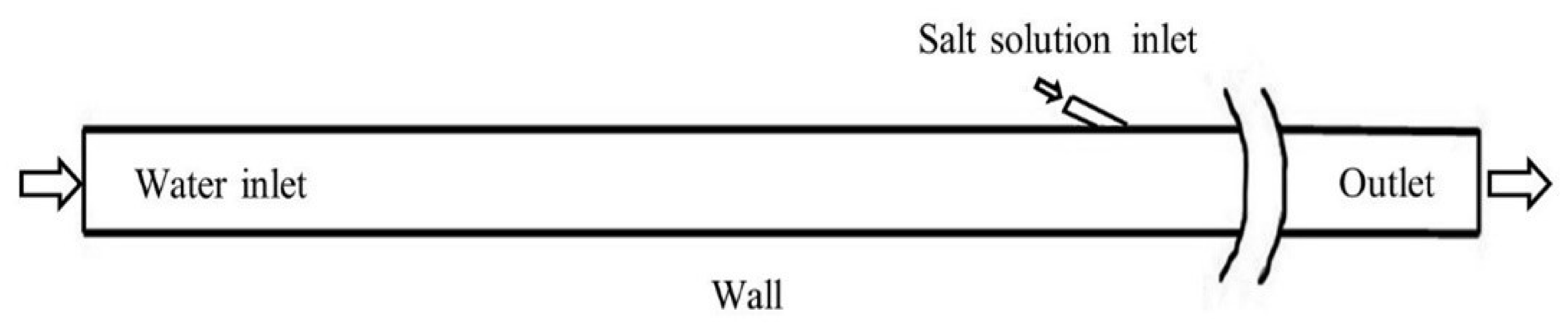
Abundant model tests were carried out and compared with numerical simulations in order to achieve the research goal [16]. The model used in this simulation consists of two parts, namely different incident angles of T-junctions (30°, 60°, 90°, 120°, 150°) and main pipes, including water inlet, salt solution inlet, the wall of pipelines, and mixture outlet. An example shape of the computational domain is shown in Figure 1.
2.1. Mathematical Model
For the simulation of turbulent characteristics in a T-junction system, the Reynolds Average Navier–Stokes equations for compressible flows are shown as the following equation [17]:
and
where is filtered velocity component, is pressure, represents gravitational body force, is the liquid density, denotes the stress tensor due to molecular viscosity and signifies the subgrid-scale stress.
2.2. Computational Grid
As shown in Figure 2, the mesh has unstructured mesh forming tetrahedral elements. Mesh size usually affects the accuracy and time taken for the calculation. Firstly, the coarse mesh may lead to a singular solution, and the mesh size should be small, which is an important prerequisite to ensure the correctness of numerical simulation. Moreover, the duration of numerical simulation should be shortened as much as possible, when the accuracy is guaranteed [18]. To quantitatively compare the results with different sizes, mesh sizes of 3, 4, and 5 mm, had been used to simulate the flow field in three different pipe diameters, respectively. The differences between the solutions were not very significant, which were less than 2%. Therefore, the mesh size of 5 mm was chosen in the simulations to reduce the simulation time.
2.3. Boundary Conditions and CFD Procedures
Boundary conditions define the physical and operational characteristics of the model on its boundaries. In this study, the water inlet and the salt solution inlet were defined as velocity inlet, as well as the mixture outlet was designated as outflow. The standard wall function was utilized on the wall of pipes to model the near turbulent flow region. The geometry of computational domain with boundary conditions is shown in Figure 1.
For turbulent flow, the turbulent intensity was calculated by turbulent intensity equation [19]:
where V is average velocity of the pipes, D is characteristic length, is dynamic viscosity, is kinematic viscosity, is Reynolds number, and I is the turbulent intensity. For the turbulent kinetic model, the standard RNG model was applied and the default values of kinetic energy and dissipation rate were used [20]. The primary water phase with a density of 997.05 kg/m3 and a viscosity value of 0.089008 mPa·s and the salt solution with a density of 1007.05 kg/m3 and a viscosity value of 0.4 mPa·s, were used.
This study referred to the simulation methods of some classical fluid mechanics cases to set up the simulation process, and low simulation was carried out using a double precision, steady state model. A SIMPLE (Semi-Implicit Pressure Linked Equations) algorithm was used which used a combination of continuity and momentum equations in this work. The under-relaxation factors were retained as the default and the initial water volume fraction was set to 0 in this computational domain. Simulations were carried out for about 9000 incremental steps where a preset value of convergence criteria was generally achieved.
3. Experiment and Model Validation
3.1. Experimental Details
The crossing position of the T-junctions and pipes was 1.5 m away from the water inlet. In the design of the pipeline experimental system and working conditions, the scale effects need to be considered to simulate the real engineering conditions. In the experimental process, the flow of liquid was mainly affected by gravity and pressure, so the gravity similarity criterion and pressure similarity criterion were mainly considered to control the scale effects and design the model test, where the similarity ratios were 1. As shown in Table 1, the working conditions were designed according to the scale effects and test conditions in combination with the design flow and pipe diameter in the relevant design specifications of the sewer. For the flow in the pipe, the flow state is turbulent when the value of Re is more than 2300. In turbulent conditions, the particles are mixed with each other, the motion is disordered, and it has energy dissipation capability and diffusivity, so they have remarkable influence on the mixing of solutions in the pipes.
The Re values of some typical working conditions are listed in Table 2, which indicated the flow in the test main pipe was turbulent. Re in the main pipe rose with the increase of the flow rate and decreased with the increase of the main pipe diameter under the same other conditions. In addition, the numbers of Re in the table were large indicating obvious turbulent characteristics.
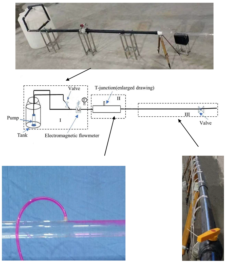
As seen in Figure 3, the experiments were conducted in a single channel flow facility, consisting of one 2000-L water tank, a 100-mm caliber electromagnetic flowmeter, several triangular supports, pumps, and different kinds of experimental pipes, valves, and so on. In this experiment, the experimental reagent was the salt solution, and the main component was sodium chloride (NaCl), which entered the experimental system from the salt solution inlet.
The water tank was used to supply a water source to the experiment, the water from the tank was pumped through the single channel at a constant flow rate, and the salt solution entered from the salt solution inlet. As the aforementioned descriptions, different branch injection angles of the T-junction were considered in the present study. The different incident angles of 30°, 60°, 90°, 120°, and 150° were designed in the test facilities. The acrylic pipes of about 2 m were used at the T-junction test section to observe the injection of salt solution, while PE pipes were used at the rest place, including the connection part. The absolute roughness of PE pipes is 0.01 mm according to the query of relevant data, and that of the test system was set during the numerical simulation to approach the material characteristics. The pipe on the front end of experimental pipes was sufficiently long to provide fully developed turbulent flow before entering the experimental pipe, at the same time the backwater pipe was designed to adjust flow rate and prevent pump damage. The inner diameter of the connection part as well as the backwater pipe was 51.4 mm, and the inner diameter of the pipe on the front end of experimental pipes was 99.4 mm. In addition, the main test pipe section was 8.5 m long and had three pipes with inner diameters of 51.4, 61.4, and 73.6 mm, respectively. One pipe was disassembled and replaced after the test.
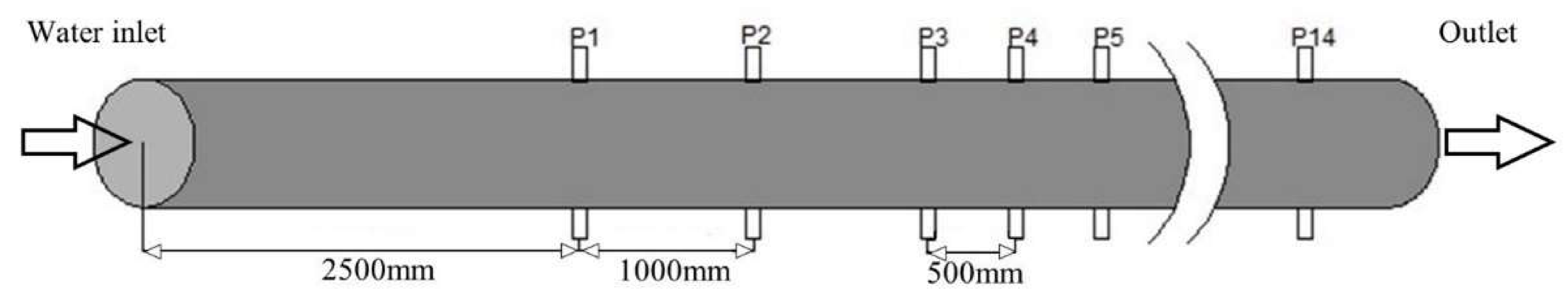
A total of 28 sampling soft rubber pipes with a diameter of about 4 mm were spaced along the direction of pipe diameter, and each group of two was arranged on the upper and lower walls of the pipe denoted as P1, P2, …, P14. Figure 4 shows the locations of the sampling soft rubber pipes. The mixed solution in each part of the experimental pipe section was collected with plastic bottles, and the electrical conductivity (EC) of the three bottles was measured and averaged. The volume fraction (VOF) of salt solution was obtained through the relationship between EC and the VOF of salt solution in the mixed solution, and then compared with the numerical simulation results to verify the accuracy of the model.
3.2. Model Validation
3.2.1. The Relationship between the Volume Fraction and Electrical Conductivity
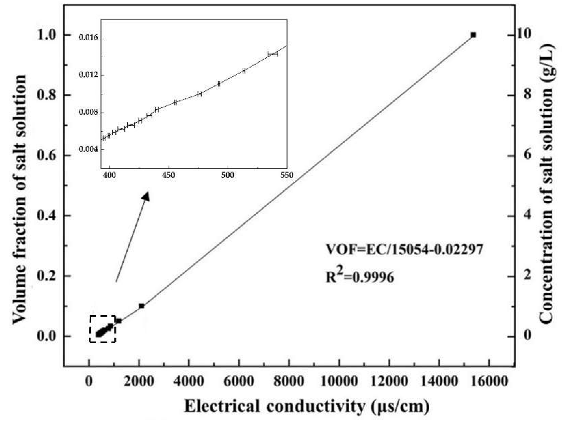
For the purpose of studying whether there is a functional relationship between the VOF of salt solution and EC, salt solutions with different concentrations (C) were prepared at the experimental temperature and their conductivity was measured synchronously. Figure 5 shows a linear relationship between EC, C, and the VOF of the salt solution. The point which the value of VOF is 1 corresponds to the conductivity of the original solution.
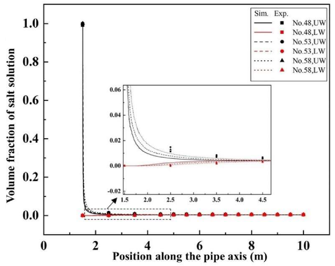
3.2.2. Comparison between Experimental Data and Simulation Results
For validating the accuracy of the model in this experiment, comparisons were carried out between the experimental data and numerical data. Figure 6 shows the comparisons of the VOF of salt solution in the upper and lower tube walls in partial experiments and simulations. As can be seen from these results that there is good agreement between them, and the results of experimental and numerical simulations have similar reasonable trends. The trends of the VOF of the salt solution on the upper tube wall (UW) decrease from large to small while those of the lower tube wall (LW) are opposite, and the trends approximately coincide at a certain position and remain stable. The maximum deviations between simulative results and experimental results are valid with the acceptable accuracy level. In conclusion, the calculation results of these numerical simulations can be applied in this study.
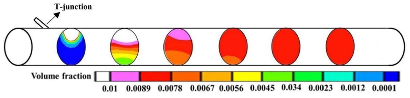
4. Results and Discussion
As shown in Figure 7, the two streams of liquid meet at the T-junction and gradually mix evenly along the main pipe centerline. In this section, the numerical data of longitudinal sections was extracted, COV [21] was used to determine the degree of mixing, which can compare the discrete degree of data well for eliminating the influence of measurement scale and dimension, defined as the mixing index:
where σ is the standard deviation of the VOF of salt solution on longitudinal sections of pipes, is the average value of the COV of salt solution, and the mixing was considered to be completely uniform when the value of COV was less than 0.05 [22]. The distance from the salt solution inlet to the fully mixed position was defined as the effective mixing length, or ‘LEML’ for short which was determined [23].
4.1. Influence Factors in the Mixing Process
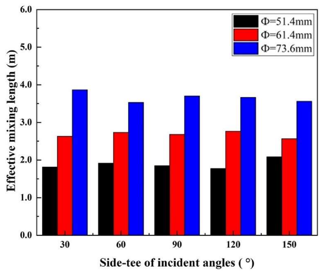
4.1.1. The Effect of Pipe Diameter on Mixing Effect
Figure 8 shows the effect of main pipe diameter φ on the mixing effect with virtually identical mixing ratio (δ = 1%), cross-flow flux (Q = 8 m3/h), and incident angles, and it can be observed that LEML increases obviously with the increase of the pipe diameter. Firstly, the area of pipe sections is reduced with the significant reduction in the pipe diameter, the salt solution diffuses more easily, and mixing time decreases significantly which leads to a shorter observed LEML. Meanwhile, increased water inlet area reduces the average flow velocity by the reason of constant cross-flow flux. The Reynolds number of a fluid with a lower velocity is a smaller result in the indistinctive characteristics of turbulent flow and the LEML increased when the impact dispersion fluidity became weak.
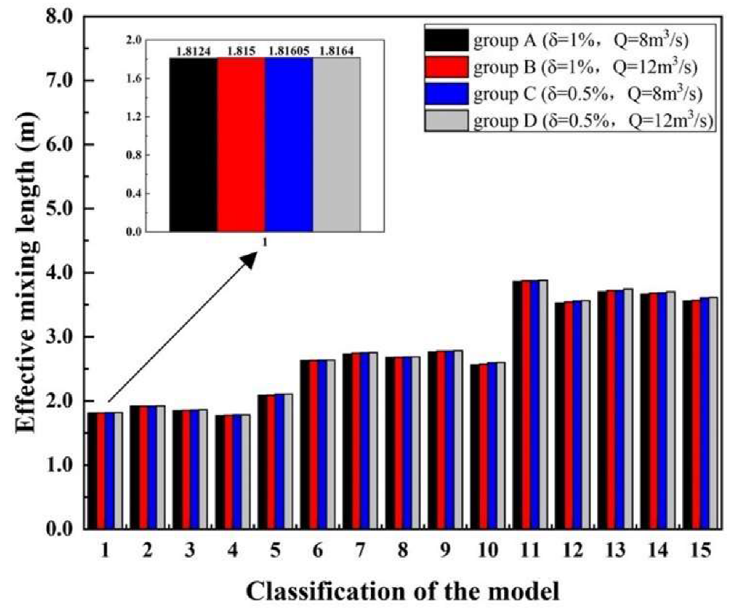
4.1.2. The Effects of Cross-Flow Flux and Mixing Ratio on Mixing Effect
Figure 9 shows the effects of cross-flow flux and mixing ratio on LEML. It can be observed that the LEML augments with the increase of cross-flow flux when other conditions remain the same, and increases when the mixing ratio is decreased. However, the effects of cross-flow flux and mixing ratio are minimal. Similar to the law of LEML with the pipe diameter, the salt solution velocity increases when raising the mixing ratio, which results in the augment of the diffusion rate of salt solution and the enhanced salt solution mixing effect to decrease the LEML.
A longitudinal section was selected for the position of 8 mm behind the T-junction to extract the region where the VOF of salt solution was more than 5%. As shown in Figure 10, the average velocities of mixed solution, water, and salt solution in the region are derived, and it can be observed that the flow rate and direction of salt solution into the main pipe are obviously affected by the water. Other things being equal, the raised water velocity by the cross-flow flux leads to the increase of the horizontal velocity of the salt solution, so that the horizontal distance of the salt solution is increased. Although the increase of velocity led to more violent mixing and accelerated the mixing of the solution, the effect was relatively small so that LEML still increased.
4.1.3. The Effect of Incident Angle of T-Junction on Mixing Effect
According to the analysis of the numerical simulation results, the incident angle is one parameter influencing the mixing characteristics in this model. As shown in Table 3, it is found that the change processes of LEML which vary with the incident angles of T-junctions differ under different main pipe diameters.
As mentioned above, a longitudinal section was cut from the position where there was a distance of 8 mm behind the junction of a T-junction and the area with the VOF of the salt solution above 5% was selected. The contours of the distribution of the salt solution and water velocity in the region are shown in Figure 11. It can be clearly seen that the VOF of the salt solution near the wall is relatively large when it just enters the main pipe, and the distribution of water velocity in the near-wall flow field is extremely uneven with a long span. In addition, the water velocity distribution is different for different pipe diameters. On account of the enormous effect of water velocity to the horizontal velocity of salt solution, the change law of LEML with the incident angles of T-junctions differ under different main pipe diameters. In the next section, the dimensional analysis (D-A) was adopted to further research the influences of the four variables on LEML.
4.2. Dimensional Analysis of Effective Mixing Length
Dimensional analysis can be used to analyze the correlation between the influencing factors and the physical variables, to solve the criterion relationship when problems cannot be described by a differential equation [24]. For clarifying the structural relationship and exploring the significant level of each variable on LEML in the structural formula, dimensional analysis was used to fit the computational expressions of LEML. Based on a thorough understanding of the research, the main physical quantities affecting the physical process must be correctly determined, to ensure the correct application of dimensional analysis. In this section, a total of eight physical quantities were considered, including effective mixing length (LEML), main pipe diameter (φ) and cross-flow flux (Q), water density (ρ), mixing ratio (), gravitational acceleration (g), incident angle (θ), and average pressure of the mixture (p).
where φ, g, and ρ are the basic physical quantities, , θ are the dimensionless quantities. As shown below, were used to represent eight proportional coefficients. Among them, , , , were formulated.
Further, the following relationships were obtained.
Substituting Equation (9) into Equation (10), a general equation can be obtained.
where a, b, c, d, and e are coefficients.
The coefficients and criterion equation were obtained by means of multivariate nonlinear regression analysis of numerical simulation data.
where LEML is effective mixing length, φ represents main pipe diameter, Q is cross-flow flux, g is gravitational acceleration, p denotes average pressure of the mixture, ρ is water density, δ signifies mixing ratio, and θ is incident angle.
Equation (12) can be transformed into the following form.
Through Equation (13) and correlation analysis, it can be seen that LEML is less affected by δ and θ which can be ignored, and affected by Q, φ, p, ρ, g dramatically. In order to simplify the calculation process, δ0.00491 and θ−0.00297 were assigned a value of 1, and the coefficients were simplified simultaneously. The simplified equation is shown below.
Comparison between the simulation results and the calculation results of Equation (14) showed that the maximum relative error was 9.56%, the minimum relative error was 0.09%, and the average error was 4.01%. According to the above error analysis, the calculation results of Equation (14) were in good agreement with the research data, which proves that the equation has high calculation accuracy and can provide guidance for the actual projects.
5. Conclusions
Due to the low design standards of some cities and the existence of extreme weather, the flow of rainwater and sewage is much higher to fill the sewers during the operation of the sewers which will lead to excessive pressure in the pipes, causing the pipes to fracture and potential collapse. A massive amount of pollutants accumulated on the urban ground surface is washed into sewers and the receiving water of the city through the collapse point, resulting in pipeline corrosion and point source pollution which can be regarded as turbulent mixing.
In this work, a CFD study of turbulent mixing in a T-junction system was performed comparing with the experimental results. The influences of main pipe diameter, mixing ratio, cross-flow flux, and incident angle on LEML were studied by the controlling variable method. The results show that the value of LEML increases as Q or φ rise and decreases with the augment of δ, of which φ has a much greater magnitude than Q and δ. Meanwhile, θ has no clear influence on LEML. Furthermore, dimensional analysis was employed to study these influences, and a dimensionless relationship equation in the harmony of dimension was obtained. Moreover, a simplified equation with the average error of 4.01% was derived, proving the applicability of it. This study provides a valuable reference to the turbulent mixing law in a T-junction system, and has broad engineering significance for tracking the origin of sewage in pipelines.
Author Contributions
Conceptualization and methodology, B.S., H.F. and C.Z.; software, formal analysis, and writing-original draft preparation, Q.L.; writing—review and editing, B.S. and C.Z.; supervision, funding acquisition, and project administration, B.S., H.F. and Y.L.; data curation, Q.L. and S.Z. All authors have read and agreed to the published version of the manuscript.
Funding
This work was supported by the National Key Research and Development Program of China (No.2017YFC1501204), the National Natural Science Foundation of China (No.51678536, 51978630, 51909242), the Program for Science and Technology Innovation Talents in Universities of Henan Province (Grant No.19HASTIT043), the Outstanding Young Talent Research Fund of Zhengzhou University (1621323001). The authors would like to give thanks for these financial supports.
Conflicts of Interest
The authors declare no conflict of interest.
References
- Jiang, G.M.; Keller, J.; Bond, P.L. Determining the long-term effects of H2S concentration, relative humidity and air temperature on concrete sewer corrosion. Water Res. 2014, 65, 157–169. [Google Scholar] [CrossRef] [PubMed] [Green Version]
- Stanev, V.G.; Iliev, F.L.; Hansen, S.; Vesselinov, V.V.; Alexandrov, B.S. Identification of release sources in advection-diffusion system by machine learning combined with Green’s function inverse method. Appl. Math. Model. 2018, 60, 64–76. [Google Scholar] [CrossRef]
- Hartmann, J.; van der Aa, M.; Wuijts, S.; Husman, A.M.D.; van der Hoek, J.P. Risk governance of potential emerging risks to drinking water quality: Analysing current practices. Environ. Sci. Policy 2018, 84, 97–104. [Google Scholar] [CrossRef]
- Wang, M.J.; Fang, D.; Xiang, Y.; Fei, Y.; Wang, Y.; Ren, W.Y.; Tian, W.X.; Su, G.H.; Qiu, S.Z. Study on the coolant mixing phenomenon in a 45 degrees T junction based on the thermal-mechanical coupling method. Appl. Therm. Eng. 2018, 144, 600–613. [Google Scholar] [CrossRef]
- Galeazzo, F.C.C.; Donnert, G.; Cardenas, C.; Sedlmaier, J.; Habisreuther, P.; Zarzalis, N.; Beck, C.; Krebs, W. Computational modeling of turbulent mixing in a jet in crossflow. Int. J. Heat Fluid Flow 2013, 41, 55–65. [Google Scholar] [CrossRef]
- Uyanwaththa, A.; Malalasekera, W.; Hargrave, G.; Dubal, M. Large Eddy Simulation of Scalar Mixing in Jet in a Cross-Flow. J. Eng. Gas Turbines Power Trans. ASME 2019, 141, 13. [Google Scholar] [CrossRef] [Green Version]
- Frank, T.; Lifante, C.; Prasser, H.M.; Menter, F. Simulation of turbulent and thermal mixing in T-junctions using URANS and scale-resolving turbulence models in ANSYS CFX. Nucl. Eng. Des. 2010, 240, 2313–2328. [Google Scholar] [CrossRef] [Green Version]
- Jayaraju, S.T.; Komen, E.M.J.; Baglietto, E. Suitability of wall-functions in Large Eddy Simulation for thermal fatigue in a T-junction. Nucl. Eng. Des. 2010, 240, 2544–2554. [Google Scholar] [CrossRef]
- Tong-Miin, L.; Chin-Chun, L.; Shih-Hui, C.; Hsin-Ming, L. Study on side-jet injection near a duct entry with various injection angles. Trans. ASME J. Fluids Eng. 1999, 121, 580–587. [Google Scholar]
- Zughbi, H.D.; Khokhar, Z.H.; Sharma, R.N. Mixing in pipelines with side and opposed tees. Ind. Eng. Chem. Res. 2003, 42, 5333–5344. [Google Scholar] [CrossRef]
- Zughbi, H.D. Effects of jet protrusion on mixing in pipelines with side-tees. Chem. Eng. Res. Des. 2006, 84, 993–1000. [Google Scholar] [CrossRef]
- Lin, C.H.; Chen, M.S.; Ferng, Y.M. Investigating thermal mixing and reverse flow characteristics in a T-junction by way of experiments. Appl. Therm. Eng. 2016, 99, 1171–1182. [Google Scholar] [CrossRef]
- Chen, M.S.; Hsieh, H.E.; Ferng, Y.M.; Pei, B.S. Experimental observations of thermal mixing characteristics in T-junction piping. Nucl. Eng. Des. 2014, 276, 107–114. [Google Scholar] [CrossRef]
- Hosseini, S.M.; Yuki, K.; Hashizume, H. Classification of turbulent jets in a T-junction area with a 90-deg bend upstream. Int. J. Heat Mass Transf. 2008, 51, 2444–2454. [Google Scholar] [CrossRef]
- Hekmat, M.H.; Saharkhiz, S.; Izadpanah, E. Investigation on the thermal mixing enhancement in a T-junction pipe. J. Braz. Soc. Mech. Sci. Eng. 2019, 41, 11. [Google Scholar] [CrossRef]
- Wang, S.J.; Mujumdar, A.S. Flow and mixing characteristics of multiple and multi-set opposing jets. Chem. Eng. Process. Process Intensif. 2007, 46, 703–712. [Google Scholar] [CrossRef]
- Ayhan, H.; Sokmen, C.N. CFD modeling of thermal mixing in a T-junction geometry using LES model. Nucl. Eng. Des. 2012, 253, 183–191. [Google Scholar] [CrossRef]
- Rahmani, R.K.; Keith, T.G.; Ayasoufi, A. Numerical simulation and mixing study of pseudoplastic fluids in an industrial helical static mixer. J. Fluids Eng. Trans. ASME 2006, 128, 467–480. [Google Scholar] [CrossRef]
- Anselmet, F.; Ternat, F.; Amielh, M.; Boiron, O.; Boyer, P.; Pietri, L. Axial development of the mean flow in the entrance region of turbulent pipe and duct flows. Comptes Rendus Mécanique 2009, 337, 573–584. [Google Scholar] [CrossRef]
- Vijiapurapu, S.; Cui, J. Performance of turbulence models for flows through rough pipes. Appl. Math. Model. 2010, 34, 1458–1466. [Google Scholar] [CrossRef]
- Rahmani, R.K.; Keith, T.G.; Ayasoufi, A. Three-dimensional numerical simulation and performance study of an industrial helical static mixer. J. Fluids Eng.Trans. ASME 2005, 127, 467–483. [Google Scholar] [CrossRef] [Green Version]
- Kamide, H.; Igarashi, M.; Kawashima, S.; Kimura, N.; Hayashi, K. Study on mixing behavior in a tee piping and numerical analyses for evaluation of thermal striping. Nucl. Eng. Des. 2009, 239, 58–67. [Google Scholar] [CrossRef]
- Vondricka, J.; Lammers, P.S. Optimization of direct nozzle injection system’s response time. In Proceedings of the Conference on Agricultural Engineering, Dusseldorf, Germany, 9–10 November 2007; pp. 507–512. [Google Scholar]
- Sonin, A.A. A generalization of the II-theorem and dimensional analysis. Proc. Natl. Acad. Sci. USA 2004, 101, 8525–8526. [Google Scholar] [CrossRef] [PubMed] [Green Version]
Figure 1.
Computational domain in two dimensional views.

Figure 2.
Typical mesh distribution in simulation of T-junction with φ = 51.4 mm, θ = 30°. (a) Side view, (b) cross-sectional view, and (c) 3-D view.
Figure 2.
Typical mesh distribution in simulation of T-junction with φ = 51.4 mm, θ = 30°. (a) Side view, (b) cross-sectional view, and (c) 3-D view.

Figure 3.
Schematic diagram of the model test layout accompanied by some photographs.

Figure 4.
Scheme on the distribution of the sampling soft rubber pipes.

Figure 5.
Relationship among electrical conductivity (EC), volume fraction (VOF), and concentration (C) of salt solution.
Figure 5.
Relationship among electrical conductivity (EC), volume fraction (VOF), and concentration (C) of salt solution.

Figure 6.
Comparison of experimental and simulation results for No. 48, No. 53, and No. 58.

Figure 7.
Section contour of the volume fraction of salt solution in the pipeline.

Figure 8.
Variation tendency of LEML under three kinds of main pipe diameters: φ = 51.4 mm; φ = 61.4 mm; φ = 73.6 mm.
Figure 8.
Variation tendency of LEML under three kinds of main pipe diameters: φ = 51.4 mm; φ = 61.4 mm; φ = 73.6 mm.

Figure 9.
Variation tendency of LEML under different cross-flow fluxes and mixing ratios.

Figure 10.
The average cross section velocities of mixture, water, and salt solution in the selected region.
Figure 10.
The average cross section velocities of mixture, water, and salt solution in the selected region.

Figure 11.
Contours of the distribution of salt solution (a) and water velocity (b) in the selected region.
Figure 11.
Contours of the distribution of salt solution (a) and water velocity (b) in the selected region.


Table 1.
Working conditions of the proposed design.
| No. | δ | Q (m3/h) | φ (mm) | θ (°) | No. | δ | Q (m3/h) | φ (mm) | θ (°) |
|---|---|---|---|---|---|---|---|---|---|
| 1 | 30 | 31 | 30 | ||||||
| 2 | 60 | 32 | 60 | ||||||
| 3 | 51.4 | 90 | 33 | 51.4 | 90 | ||||
| 4 | 120 | 34 | 120 | ||||||
| 5 | 150 | 35 | 150 | ||||||
| 6 | 30 | 36 | 30 | ||||||
| 7 | 60 | 37 | 60 | ||||||
| 8 | 8 | 61.4 | 90 | 38 | 8 | 61.4 | 90 | ||
| 9 | 120 | 39 | 120 | ||||||
| 10 | 150 | 40 | 150 | ||||||
| 11 | 30 | 41 | 30 | ||||||
| 12 | 60 | 42 | 60 | ||||||
| 13 | 73.6 | 90 | 43 | 73.6 | 90 | ||||
| 14 | 120 | 44 | 120 | ||||||
| 15 | 1% | 150 | 45 | 0.5% | 150 | ||||
| 16 | 30 | 46 | 30 | ||||||
| 17 | 60 | 47 | 60 | ||||||
| 18 | 51.4 | 90 | 48 | 51.4 | 90 | ||||
| 19 | 120 | 49 | 120 | ||||||
| 20 | 150 | 50 | 150 | ||||||
| 21 | 30 | 51 | 30 | ||||||
| 22 | 60 | 52 | 60 | ||||||
| 23 | 12 | 61.4 | 90 | 53 | 12 | 61.4 | 90 | ||
| 24 | 120 | 54 | 120 | ||||||
| 25 | 150 | 55 | 150 | ||||||
| 26 | 30 | 56 | 30 | ||||||
| 27 | 60 | 57 | 60 | ||||||
| 28 | 73.6 | 90 | 58 | 73.6 | 90 | ||||
| 29 | 120 | 59 | 120 | ||||||
| 30 | 150 | 60 | 150 |
Table 2.
The Re value of the water flow for No. 1, No. 6, No. 11, No. 16, No. 21, No. 26.
| No | Re | No | Re | No. | Re |
|---|---|---|---|---|---|
| 1 | 616,940 | 6 | 516,461 | 11 | 430,852 |
| 16 | 925,409 | 21 | 774,691 | 26 | 646,278 |
Table 3.
Comparison of LEML under different diameters and incident angles.
| Diameter (mm) | Incident Angle | LEML of Group A (m) | LEML of Group B (m) | LEML of Group C (m) | LEML of Group D (m) |
|---|---|---|---|---|---|
| 30° | 1.8124 | 1.8150 | 1.8161 | 1.8164 | |
| 60° | 1.9167 | 1.9168 | 1.9172 | 1.9220 | |
| 51.4 | 90° | 1.8496 | 1.8520 | 1.8599 | 1.8610 |
| 120° | 1.7747 | 1.7753 | 1.7796 | 1.7800 | |
| 150° | 2.0830 | 2.0879 | 2.1070 | 2.1090 | |
| 30° | 2.6286 | 2.6345 | 2.6347 | 2.6353 | |
| 60° | 2.7339 | 2.7450 | 2.7520 | 2.7549 | |
| 61.4 | 90° | 2.6790 | 2.6830 | 2.6850 | 2.6882 |
| 120° | 2.7638 | 2.7754 | 2.7769 | 2.7804 | |
| 150° | 2.5650 | 2.5752 | 2.5970 | 2.5990 | |
| 30° | 3.8650 | 3.8710 | 3.8740 | 3.8790 | |
| 60° | 3.5270 | 3.5402 | 3.5600 | 3.5632 | |
| 73.6 | 90° | 3.7007 | 3.7208 | 3.7240 | 3.7439 |
| 120° | 3.6640 | 3.6808 | 3.6868 | 3.7010 | |
| 150° | 3.5600 | 3.5680 | 3.6092 | 3.6120 |
© 2020 by the authors. Licensee MDPI, Basel, Switzerland. This article is an open access article distributed under the terms and conditions of the Creative Commons Attribution (CC BY) license (http://creativecommons.org/licenses/by/4.0/).
Share and Cite
MDPI and ACS Style
Sun, B.; Liu, Q.; Fang, H.; Zhang, C.; Lu, Y.; Zhu, S. Numerical and Experimental Study of Turbulent Mixing Characteristics in a T-Junction System. Appl. Sci. 2020, 10, 3899. https://doi.org/10.3390/app10113899
AMA Style
Sun B, Liu Q, Fang H, Zhang C, Lu Y, Zhu S. Numerical and Experimental Study of Turbulent Mixing Characteristics in a T-Junction System. Applied Sciences. 2020; 10(11):3899. https://doi.org/10.3390/app10113899
Chicago/Turabian StyleSun, Bin, Quan Liu, Hongyuan Fang, Chao Zhang, Yuanbo Lu, and Shun Zhu. 2020. "Numerical and Experimental Study of Turbulent Mixing Characteristics in a T-Junction System" Applied Sciences 10, no. 11: 3899. https://doi.org/10.3390/app10113899
Note that from the first issue of 2016, this journal uses article numbers instead of page numbers. See further details here.