May a Standard VOF Numerical Simulation Adequately Complete Spillway Laboratory Measurements in an Operational Context? The Case of Sa Stria Dam


1
DICAAR, University of Cagliari, 09123 Cagliari, Italy
2
RED Fluid Dynamics, 47921 Rimini, Italy
*
Author to whom correspondence should be addressed.
Water 2020, 12(6), 1606; https://doi.org/10.3390/w12061606
Submission received: 13 May 2020
/
Revised: 27 May 2020
/
Accepted: 29 May 2020
/
Published: 4 June 2020
(This article belongs to the Special Issue Planning and Management of Hydraulic Infrastructure)
Abstract
:The present work aims to assess whether a standard numerical simulation (RANS-VOF model with closure) can adequately model experimental measurements obtained in a dam physical model. The investigation is carried out on the Sa Stria Dam, a roller compacted concrete gravity dam currently under construction in Southern Sardinia (Italy). The original project, for which a physical model was simulated, included a downstream secondary dam. However, due to both economic and technical reasons, the secondary dam may not be built. Hence, it is important to assess the flood discharge routing and energy dissipation in the modified plan. Numerical validation is performed adopting the same laboratory configuration, in presence of the downstream dam, and results show a good agreement with mean experimental variables (i.e., pressure, water level). An alternative configuration without the downstream dam is here numerically tested to understand the conditions of flood discharge and assess whether its results can give relevant information for the design of mitigation measures. The topic is of interest also from a more general perspective. Indeed, the feasibility to integrate numerical models with existing laboratory measurements can be very useful not only for new constructions but also for existing dams, which may need either maintenance or upgrading works, such as in case of flood discharge increment.
1. Introduction
The design and safety assessment of the discharge structures of dams have always relied upon physical models, which are still irreplaceable for evaluating overflow discharge and flood energy downstream dissipation. Nonetheless, thanks to the continuous advancements in numerical modelling, the synergistic integration of computational fluid dynamics (CFD) and laboratory simulations may certainly be foreseen as a standard operative tool within the dam engineering field.
One of the first examples of numerical simulation applied to dam modelling was by [1] who computed the flow over a spillway with a 3D RANS (Reynolds Averaged Navier Stokes)model. Successively, many studies have been devoted to both the development and testing of numerical models in this context (see the review article by [2] and references therein). Indeed, parallel to these methodological works, investigations on case studies are important to understand the feasibility to apply numerical methods to a field traditionally investigated only with physical modelling. Numerical simulations have been applied in different parts of the world. For instance, Cook and coauthors used numerical modelling to improve the spillway of the Dalles Dam, in the Columbia River [3]. A review of the spillway upgrade projects performed in Australia with the aid of CFD is reported in [4]. Reference [5] compared experimental and numerical simulations to an upgraded spillway of an Indian dam, demonstrating how the numerical model can capture the water surface profile along the spillway very accurately, and can be a complementary tool for assessing the hydraulic performance of structures. Reference [6] used a 3D hydrodynamic model to unveil safety issues in an Ethiopian dam spillway. In addition, Reference [7], after a review of Sweden dams, highlights the potentiality of CFD to be used in conjunction with physical modelling.
This kind of case-studies are very important to increase CFD testing and widen the dam engineering community awareness in this field. Indeed, physical simulations have been used in dam modelling for over 100 years, whilst the numerical methods for spillways have been under development from the 1970s but, at first, only for research purposes. Hence, CFD application in dam engineering has been subject to much less testing than physical modelling in real cases. Indeed, both experimental and numerical modelling present strengths and weaknesses. Physical models have higher costs and are more time consuming both in building the model and in the measurement campaigns. Numerical models provide a full knowledge of all the variables in the computational domain, which is not possible to achieve with experimental techniques. However, CFD models suffer from underlying hypotheses and have to be properly validated against physical models. If simulations are performed at the prototype scale, numerical results are not affected by scale effects that always occur in physical models. Moreover, CFD models are more flexible and allow to quickly create and analyse the hydraulic behaviour within different scenarios for existing structures as well as for new ones. Indeed, they are extremely useful in the earliest steps of the design process to select the configurations to test with physical modelling or to evaluate secondary modifications to existing dams.
The present work focuses on the Sa Stria Dam, a roller compacted concrete gravity dam at present under construction in Southern Sardinia (Italy) and numerically investigates the impact of a possible design modification. As better detailed in the following section, a secondary stepped dam was originally planned downstream of the main dam, but its construction is at present in doubt. Here, the results of the physical model carried out at the Padua University (Italy) according to the original project are used to validate a numerical model, which is then used to assess the consequences of the flood discharge throughout the river valley without the stilling basin formed by the secondary dam. A standard application of the volume of fluid (VOF) technique with the turbulence model is performed under a public domain code, OpenFOAM®, in order to test whether a standard simulation can adequately integrate laboratory experiments.
Although the present work is focused on a specific case study, and thus the encouraging results hereby discussed cannot be generalised, they are nonetheless a step forward in the existing literature panorama. They show how numerical simulations can be utilised in an operative context, in order to integrate laboratory models and to explore new project configurations or secondary modifications. This specific problem is indeed of the utmost modernity not just for new constructions but also for existing dams, in the case of flood discharge increment or conservative works. Indeed, also considering climate change scenarios, there may be the need for a re-evaluation of flood frequency and magnitude impacting dam safety, and plan spillway with enhanced discharge capacity [8].
The manuscript is organised as follows: Section 2 describes the case study, Section 3 the numerical method and simulations details, Section 4 validates the numerical simulation performed in presence of the secondary dam against the corresponding laboratory model, and investigates the flow modifications without the downstream dam. In Section 5 the limitations and the outcomes of the work are discussed in a more general framework.
2. Case Study
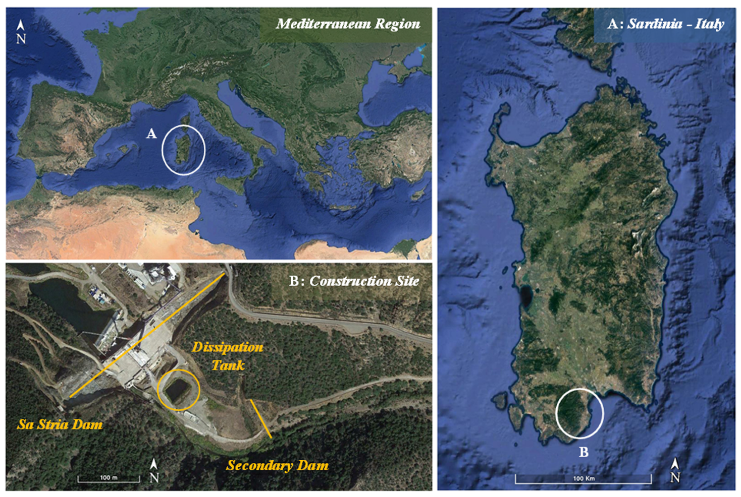
The case study here analysed is the Sa Stria Dam, which is being built in the southern part of Sardinia (Italy) (see Figure 1) and was commissioned by the local Internal Drainage Board, called the Consorzio di Bonifica della Sardegna Meridionale (CBSM). The works for its construction begun in 1998, and after a long interruption due a controversy, the construction site reopened in 2014. Sa Stria is a rolled gravity dam, 82.68 m in height; its spillway crest is divided into four bays of 11.5 m each, and its chute ends with a horizontal ski jump. Downstream of the dam, a rectangular dissipation tank, 3.20 m in depth, is planned (its location is shown in Figure 1) to guarantee the jet impingement on a deeper water cushion, thereby protecting the dam foot against erosion.
Sa Stria Dam should have been part of a wider and more complex water system that will not be completed due to both environmental and economic issues. In the original project a secondary stepped dam, 10 m high and 70 m long, was planned around 200 m downstream of the main dam (see Figure 1). This secondary structure had a twofold aim. On one side it allowed the formation of a stilling basin for water to be pumped upstream during the winter time. On the other side the presence of a deeper water cushion for the jet from the spillway had a protective role with respect to the valley bottom flood routing and utterly contributed to the water energy dissipation through the secondary dam stepped spillway. This planned configuration was tested in a laboratory model, reproduced at 1:40 scale at the Laboratory of the University of Padua (Italy) in 2001, to assess the spillway performance and energy dissipation, as requested by the Italian legislation. However, since the whole interconnected system will no longer be constructed, the secondary dam will lose its first hydraulic purpose, and the hypothesis to let the flood energy dissipate throughout the valley bottom, without the presence of a stilling basing, is currently under investigation.
It is worthwhile mentioning that the terrain both in the dam foundation area and in the downstream valley region was made of solid non-erodible rock. However, after the initial building stages, the works were interrupted for almost 15 years (from 2001 to 2015). Hence the terrain in the building site was exposed to meteorological forcing and when the building site re-opened, after a detailed geotechnical investigation campaign, extensive consolidation grouting was performed to strengthen the partially weathered rock.
Despite the solid rock foundation, the original project established a plunge pool lining of reinforced concrete slabs in the dissipation tank. If the secondary dam will not be constructed, the area and the type of reinforcement will be modified accordingly, due to the different jet impact and the higher erosion potential.
3. Materials and Methods
Numerical Model
In this study, the multiphase flow of air and water over the spillway and along the terrain downstream of the dam is modelled in the framework of unstructured finite-volume schemes with the help of the public-domain CFD code OpenFOAM® and using Reynolds-Averaged Navier–Stokes (RANS) models to account for the turbulent nature of the flow and the volume of fluid (VOF) method to model the evolution of the air/water interface. The same numerical methodology has been employed and applied successfully in the past by several researchers to the study of air and water flows over dams, spillways, air-vents and chutes [9,10,11,12].
In the VOF method [13], a single set of flow governing equations are solved for the air/water mixture by introducing the concept of the volume fraction , the ratio between the volume occupied in a single cell by the fluid and the cell volume. In the framework of RANS turbulence modelling, the governing equations of the multiphase flow, VOF-based, model read as follows:
where , , p and are the density, velocity, pressure and molecular viscosity of the air/water mixture, respectively, and the density and volume fraction of the liquid (water) phase and the turbulent viscosity.
Note the calculated flow variables (density, pressure, velocity and volume fraction) provided by the RANS Equations (1)–(3) represent mean values, but these values can fluctuate over time due to large-scale fluctuations of the free-surface flow associated with the impingement of the spillway water jet and the flow evolution along the riverbed. Such fluctuations are resolved explicitly by the present model, whereas the higher frequency/wavenumber turbulent scales are estimated via the RANS turbulence model. In the present study, the contribution of such unresolved turbulent scales on the mean flow is accounted for entirely by the turbulent viscosity . The turbulent viscosity is calculated using the model, where two additional transport equations, not reported here for the sake of brevity, are solved for the turbulent kinetic energy k and its dissipation rate .
The near-wall region of the turbulent boundary layer associated with the water flow is also fully modelled via the use of wall-functions and not resolved explicitly due to the high Reynolds number of the flow, in order to relax the mesh resolution requirement at the wall and reduce the computational effort requested by the model. At this stage, the surface roughness of the structures, such as the spillway, dissipation basin and secondary dam, as well as of the terrain and riverbed is not taken into account and thus considered hydraulically smooth.
Equations (1) and (2) are the continuity and momentum equations, respectively, and Equation (3) is the transport equation for the liquid volume fraction, which is solved in order to track the evolution of the air/water interface. Note that for a two-fluid system there is no need to solve for a transport equation of the gas (air) phase once the equation for the liquid phase is solved, since for two immiscible fluids the sum of volume fractions must equal unity and the secondary volume fraction can be obtained by subtraction once the volume fraction of the primary phase is calculated by Equation (3).
The flow governing Equations (1)–(3) are spatially solved on the computational grid using second-order accurate unstructured finite-volume schemes to allow for handling of the complex geometry characterising both the spillway and the terrain downstream. The diffusive transport terms are approximated using a central-scheme, whereas a linear upwind scheme is used for the convective transport term of the momentum Equation (2). For the convective transport term of the volume fraction Equation (3) the higher-order, Total Variation Diminishing (TVD) Monotonic Upstream-centred Scheme for Conservation Laws (MUSCL) scheme of van Leer [14] is used in order to preserve the sharpness of the air/water interface.
Temporal advancement of the flow and of the volume fraction in Equations (2) and (3) is performed using the implicit first-order accurate forward Euler scheme. In both configurations with and without the secondary dam in place, the simulations are run until a statistically steady-state regime is reached. Temporal statistics are then computed for the flow variables of interest. For the configuration with the secondary dam in place, the total simulation time at real scale is about 19 mins and the mean values and standard-deviation computed over about the last 6 mins of the simulation. The total simulation time is increased to about 27 mins for the configuration without the secondary dam, due to the time needed by the flow to cover the length of the river bed, whereas the same time window used in the configuration with the secondary dam, about 6 mins, is employed to compute the flow statistics.
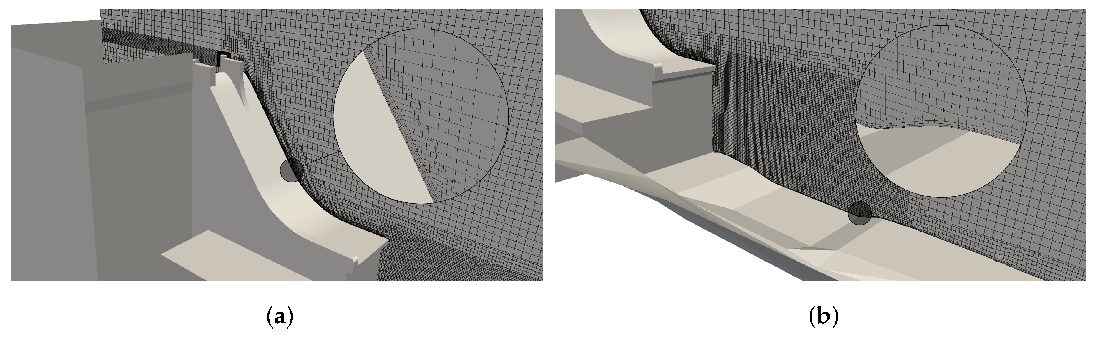
An overview of the computational grid structure and resolution in the spillway region, shared by the configurations with and without the secondary dam, is given in Figure 2a,b. A body conformal hex-dominant mesh is employed with local surface and volume refinements. The background, minimum grid resolution is 2 m at the prototype scale whereas the maximum resolution, adopted on the crest of the spillway profile, is 12.5 cm at real scale. In this region, a vertical refinement of the background grid extending horizontally over the entire feeding tank (see Figure 2a) is introduced to improve the accuracy of the predicted water level for a given discharge flow rate.
Along the main spillway surface, an isotropic grid refinement is used up to a grid resolution of 25 cm. Boundary layer-type cells are also extruded at the surface (see the circle in Figure 2a) to capture the development of the boundary layer flow along the surface accurately. The boundary layer cells are also extruded over the dissipation basin (see Figure 2b), where the grid is also isotropically refined up to 50 cm in the volume region between the basin and the spillway, as well as along the terrain and the river bed. In the configuration with the secondary dam, a grid resolution on the stair-step profile of 12.5 cm is employed. A refinement region with resolution of 50 cm across the water level of the stilling basin is also employed in this case to better capture the overflow height on top of the secondary dam.
The boundary conditions enforced in the numerical model at the inlet section of the computational domain, represented by the feeding pipe in the configuration with the secondary dam and by the vertical back surface of the feeding tank in the configuration without the secondary dam, are the discharge flow rate and a volume fraction of unity, corresponding to the liquid-phase, along with the turbulent kinetic energy and dissipation rate estimated assuming a turbulence intensity of 10% and a turbulent viscosity to molecular viscosity ratio of 10. At the top and lateral boundaries of the domain, not including the terrain slope or other solid surfaces, a free-slip condition is enforced for the velocity field whereas the total pressure is fixed at the top surface along with a zero-gradient condition on the lateral boundaries for the pressure field, also enforced for the turbulent quantities. At the exit of the computational domain, a fully developed flow condition is enforced for all variables. At the solid surfaces, including the structures of the dam and the terrain, the no-slip and zero-gradient conditions are enforced for the velocity and pressure field, respectively, whereas the value of the turbulent quantities are extrapolated using the wall-functions cited above.
4. Results
In the following sections, the results from the overflow simulations of the Sa Stria Dam with and without the downstream dam are discussed. With the secondary dam in place, the numerical model is run in the same set-up used for laboratory simulations (Section 4.1). The results are validated by comparing the water level measurements at the spillway crest and in the stilling basin, as well as of pressure measurements at the bottom of the basin and on the secondary dam. The model is then applied to the configuration without the downstream dam (Section 4.2), and the analysis is extended from the Sa Stria Dam to the flow along the riverbed. A comparison and discussion of the numerical results for the two cases is also presented, highlighting the effect of the downstream dam on the flow dynamics and characteristics downstream of the main spillway.
4.1. Simulation and Validation in Presence of the Downstream Dam
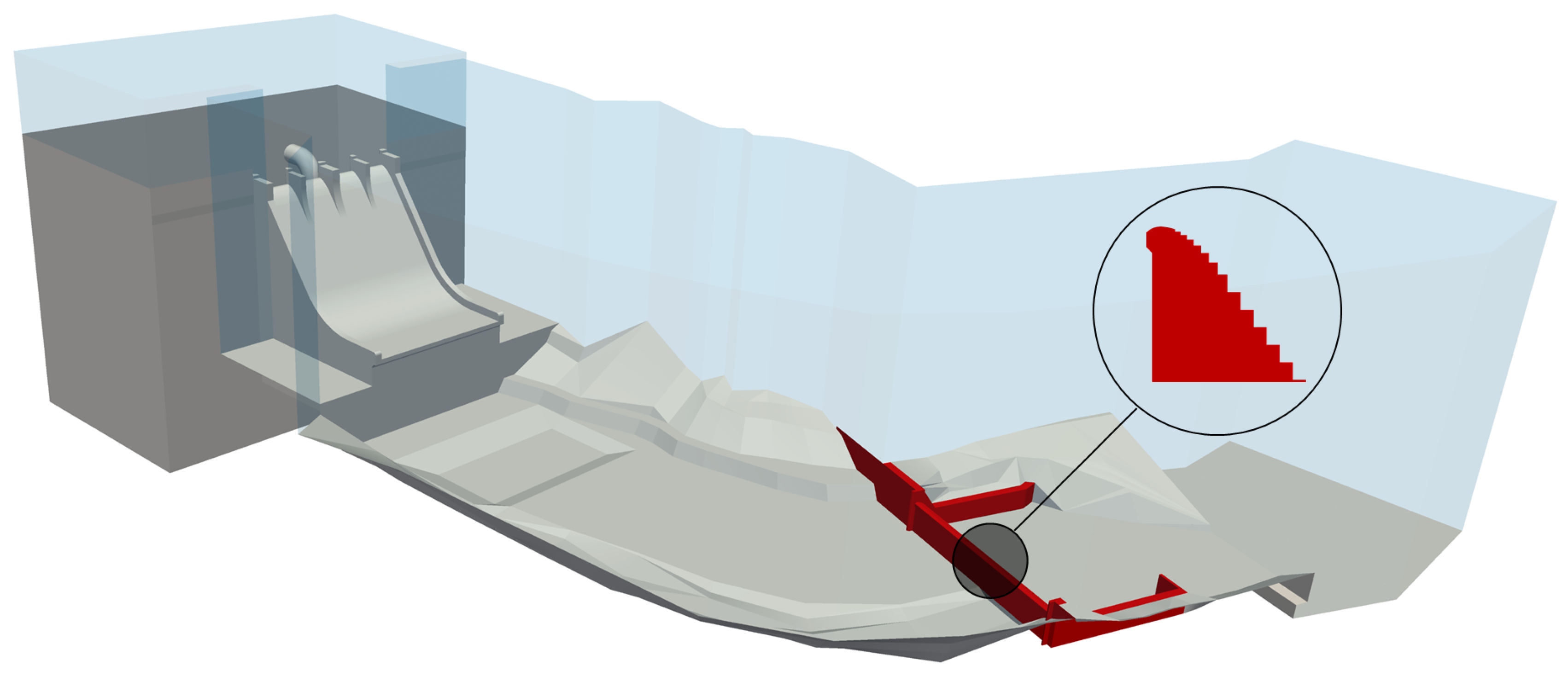
The geometry model representing the configuration with the downstream dam is presented in Figure 3. This set-up exactly corresponds to the one adopted for the physical model, and documented in the dam original project. Here, the digital model is developed starting from the available 3D CAD model of the spillway provided by CBSM, whereas the 3D model of the downstream dam and of the stilling basin are built from the 2D drawings of the laboratory set-up, also provided by CBSM. Downstream of the secondary dam, the river width narrows and a wall on the right river bank further confines the flow, forming another energy dissipation basin where an hydraulic jump will occur during flood discharge. Both the numerical and physical model end with a jump in the river bed, disconnecting the free surface profile. In order to match the experimental setup as close as possible, also the reservoir upstream of the spillway is modelled by the same tank geometry used in the physical model. The tank is served by a feeding pipe visible in Figure 3, which is directed downward to avoid unrealistic velocities in the flow entering the spillway and to prevent the onset of asymmetries. This is highlighted in Figure 4, where the magnitude and structure of the velocity field on a vertical section through the symmetry plane of the inlet pipe are shown.
The physical modelling is performed under the Froude similarity with a 1:40 scaling factor. The same conditions are chosen for the numerical model, with the aim of assessing whether it can provide an adequate description of the flow, comparable with a physical model at the same scale. The scaling factor between the small scale models (both laboratory and numerical ones) and the prototype are reported in Table 1. Note that all numerical results presented in the following are up-scaled to the prototype scale.
Since the measurements in the physical model are performed in a steady-state regime, each simulation is started with both the upstream tank at the stilling basin already filled with water, as shown in Figure 5, in order to reduce the time needed to reach the statistically steady-state condition in the simulations.
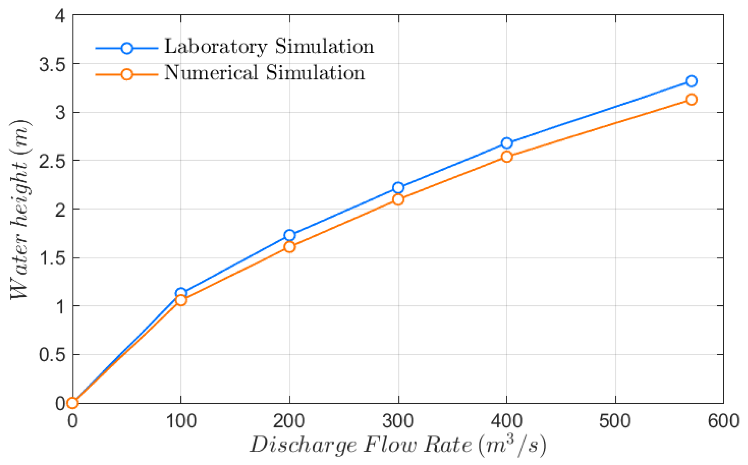
In Figure 6, the predicted water level at the spillway crest is compared to measurements for all discharge flow rates simulated with the physical model. A very good agreement with the experiments is observed, with an average deviation over all flow rates below 6%. Indeed, the underprediction of experimental data might depend on the choice of smooth wall for the spillway. However, since the main focus of the work was the downstream flow and the agreement is very satisfactory, further options were not considered.
The spillway design flood is 570 m, corresponding to about 3.1 m of overflow height over the spillway profile, but the experimental pressure measurements for this discharge rate were not available, while a more complete experimental data-set is documented for 300 m, which was therefore assumed for model validation. The validation of the numerical model is carried out by comparing the predicted water levels in the stilling basin, near the secondary dam, using two virtual hydrometers located at the corresponding positions in the physical model, also shown in Figure 5. Moreover, the predicted water pressure at several locations at the bottom of the dissipation basin, shown in Figure 7a, and along the secondary dam were also considered. Water pressure is measured locally along the downstream dam profile using probes in the physical model, whereas the time-averaged mean pressure predicted in the present RANS modelling framework is also spatially averaged on the measuring surfaces shown in Figure 7b.
The mean pressure and standard-deviation for the pressure probes in the dissipation basin, computed once the statistically-steady regime has been reached, are compared to experimental values in Table 2. In the physical model, the mean and fluctuating pressures at the bottom of the dissipation basin were obtained with pressure transducers. According to the project technical report, these have an accuracy of 0.05% in the 0–1 bar measurement range. Although there is a slight tendency of underpredicting the mean water pressure by the numerical model, the numerical values are remarkably in good agreement with measurements, with an average deviation close to 1%. The standard deviation predicted by the numerical model, however, is found severely underestimated, with an average deviation of 86% from the values measured in the physical model. This is not surprising given the inherent drawbacks of the RANS approach, which has limited capability, in general, to compute accurately the turbulent components.
A good agreement between simulations and experiments is also observed for the predicted time and spatially averaged water pressure along the stair-step profile of the secondary dam, shown in Table 3. Except for sensor 2, the average deviation of the numerical solution from measured data is found within 13%. We speculate that sensor 2 higher discrepancy might be caused by larger disturbances characterising the initial interaction of the water flow entering the stepped dam profile from the stilling basin, which may results in increased measurement uncertainty. From the remaining sensors, an increasing difference between the horizontal surfaces (surfaces 1, 3 and 5 in the numerical model) and the vertical surfaces (surfaces 2, 4 and 6 in the numerical model) can be observed in both computations and measurements, associated with the gain in dynamic pressure from the water while flowing down the stair-step profile.
The comparison between predicted and measured water levels from the two hydrometers located in proximity of the secondary dam (Figure 3) is also found satisfactory from an engineering point of view, with an average deviation of the order of 15% between the numerical and the physical model.
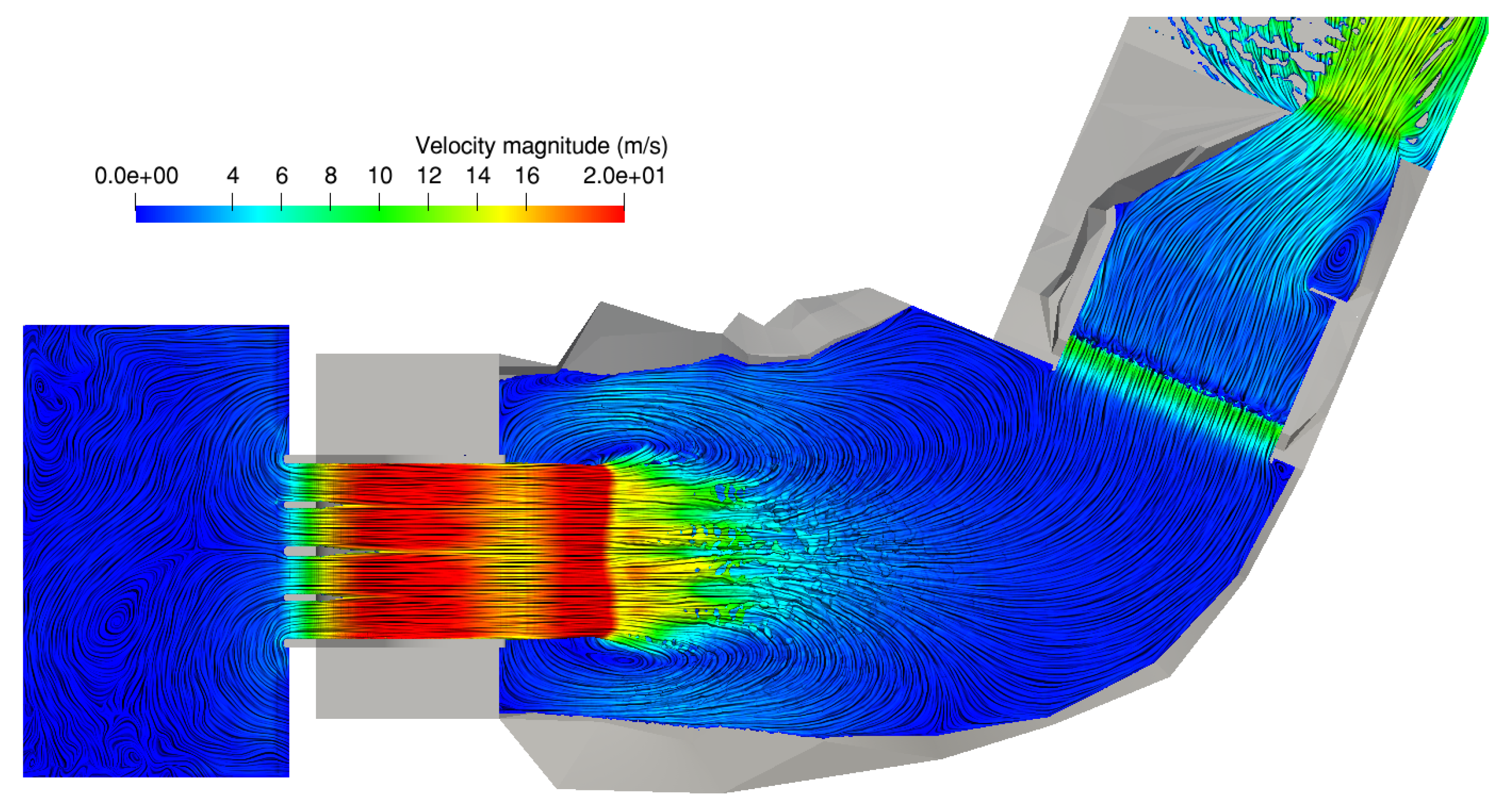
After validating the present numerical model against experimental data, flow visualisations are carried out to provide additional insight in the overflow scenario with the downstream dam in place at the same discharge flow rate. The velocity and structure characterising the water flow are presented in Figure 8. Water speed above 20 m/s at the prototype scale is observed in the accelerating flow down the spillway and in the jet zone before the impact with the stilling basin. Near the impinging region two large and symmetric recirculation zones are formed within the stilling basin, draining part of the discharge flow rate back towards the dam foot region while the bulk of the flow proceeds towards the secondary dam. The flow acceleration down the stair-step profile of the secondary dam can be clearly noticed in the figure, with water speed exceeding 10 m/s at the prototype scale, followed by the hydraulic jump occurring at the bottom of the stepped profile. Downstream of the hydraulic jump, the water speed reduces to about 3 m/s before accelerating in the end section of the computational domain, where the actual terrain is still present and characterised by a restriction in the width of the riverbed.
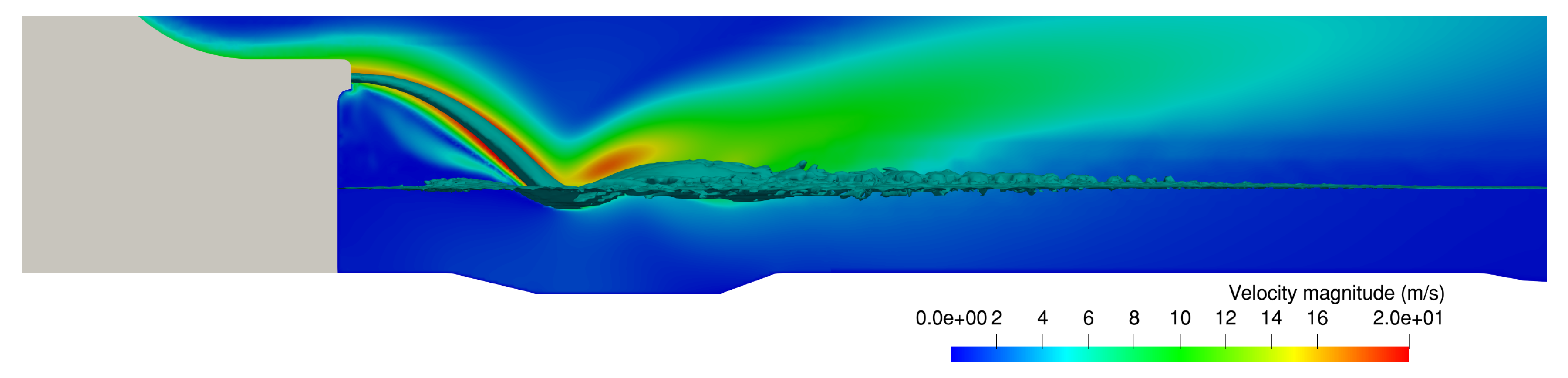
The flow structure near the impinging region is highlighted in Figure 9, where the flow speed is mapped on a vertical plane. From the visualisation of the free-surface superimposed on the image, a limited penetration of the jet in the stilling basin is apparent, even though flow velocity as high as 2 m/s can be observed beneath the surface.
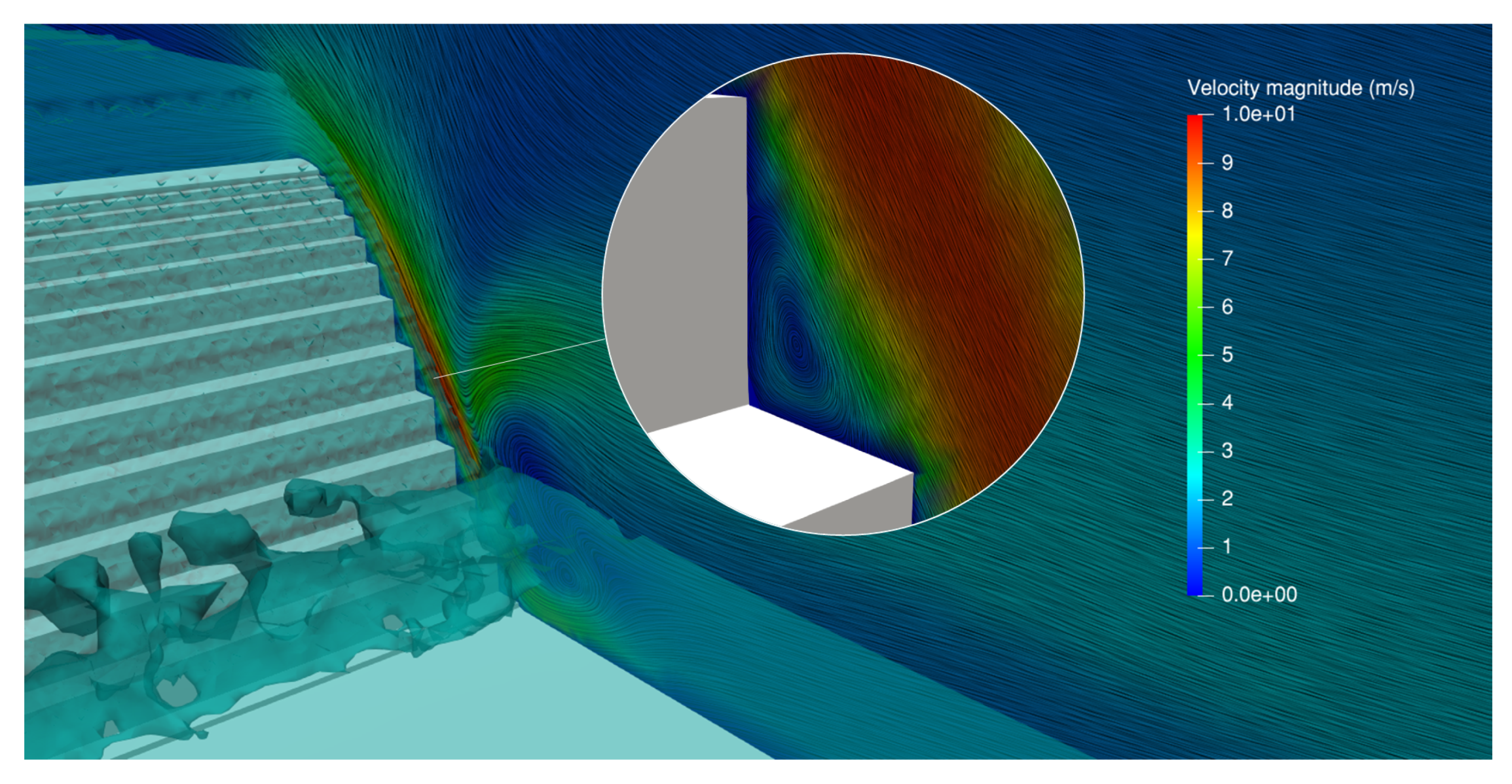
In Figure 10, the structure of the water flow along the stair-step profile of the downstream dam is finally presented. The visualisation of the free-surface clearly highlights the onset of the hydraulic jump at the bottom of the profile and the development of large scale turbulent structures. In the detailed view within the circle, the flow recirculation over each step of the profile is also shown. This witnesses how the flow dynamics is well resolved by the model, although the flow separation may be responsible for some of the uncertainty associated with pressure measurements along the secondary dam.
4.2. Simulation in Absence of the Downstream Dam
For the configuration without the downstream dam, shown in Figure 11, the same 3D model of the spillway provided by CBSM and used in the previous analysis is employed, whereas both the model of the upstream feeding tank and of the terrain are modified. Compared to the model setup including the secondary dam presented in Section 4.1, the incoming overflow is here simulated by replacing the feeding pipe with a flat inflow section, also shown in Figure 11, corresponding to the back surface of the feeding tank. This setup is chosen to provide a more uniform and consistent feeding of the spillway compared to the real scale, given the lack of reference data from the laboratory model for the configuration without the secondary dam and the successful validation of the CFD model in the original design layout. Indeed the effects of this different inlet option was proofed to be negligible on the spillway overflow.
The terrain model is also modified to include the riverbed morphology downstream of the designed location for the secondary dam. In the upstream region, where the stilling basin would be formed for the secondary dam set-up, the terrain is very similar to the previous configuration but obtained, in this case, via georeferenced maps provided by CBSM. Note the dissipation tank is included in the maps and thus is still present in this configuration.
For the present layout, the simulations are initiated with empty terrain and empty riverbed downstream of the spillway and run until a statistically steady-state is reached. As in the previous configuration, several virtual probes are used to monitor the numerical solution and verify the achievement of a statistically steady state.
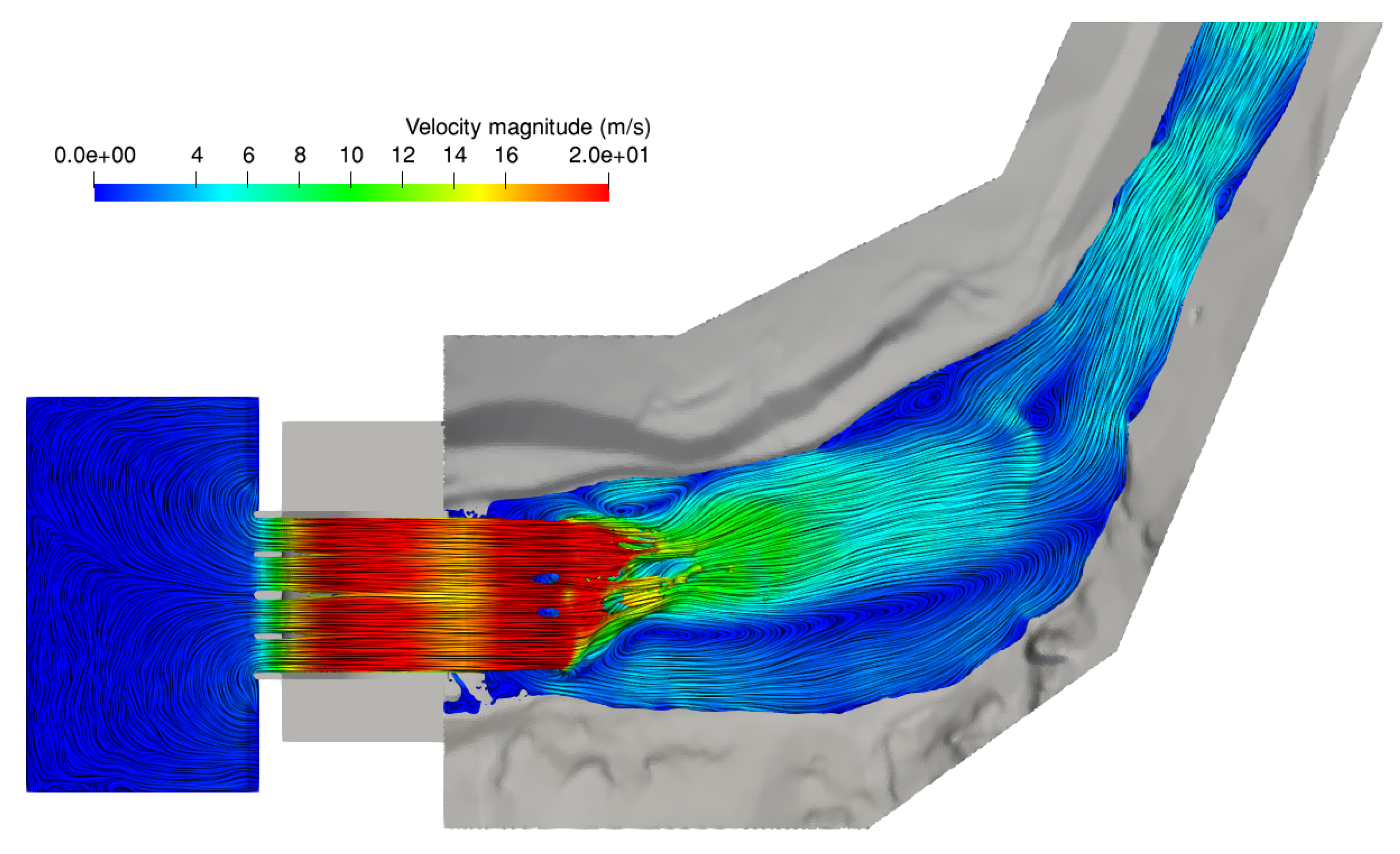
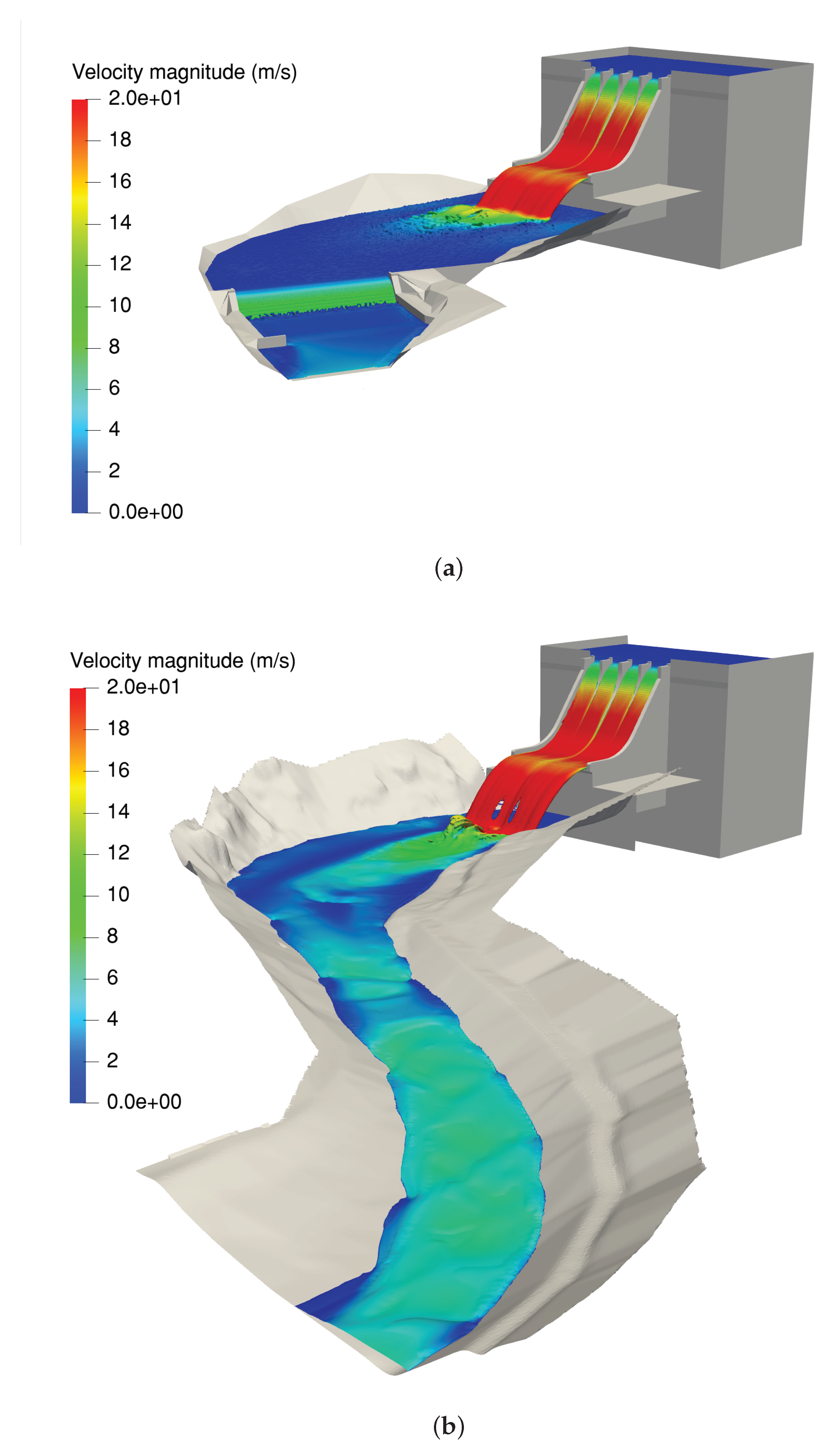
The overall structure and speed of the water flow is presented in Figure 12 for discharge flow rate of 300 m. The flow structure at the ground is characterised by a sharp deflection to the left side of the basin right after the impact of the water jet with the terrain. This causes a very large recirculating region within the right side of the basin, where the flow moves upstream back towards the spillway. A smaller recirculating region can be also noticed on the left side of the basin as well as the formation of two main currents right before the flow enters the riverbed.
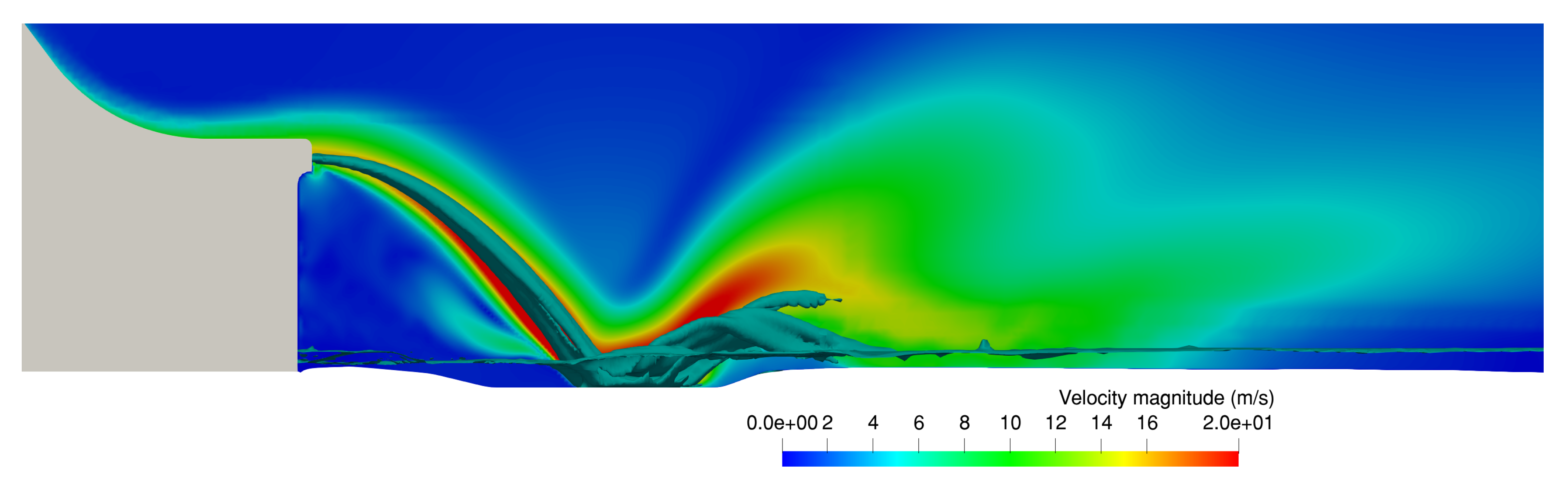
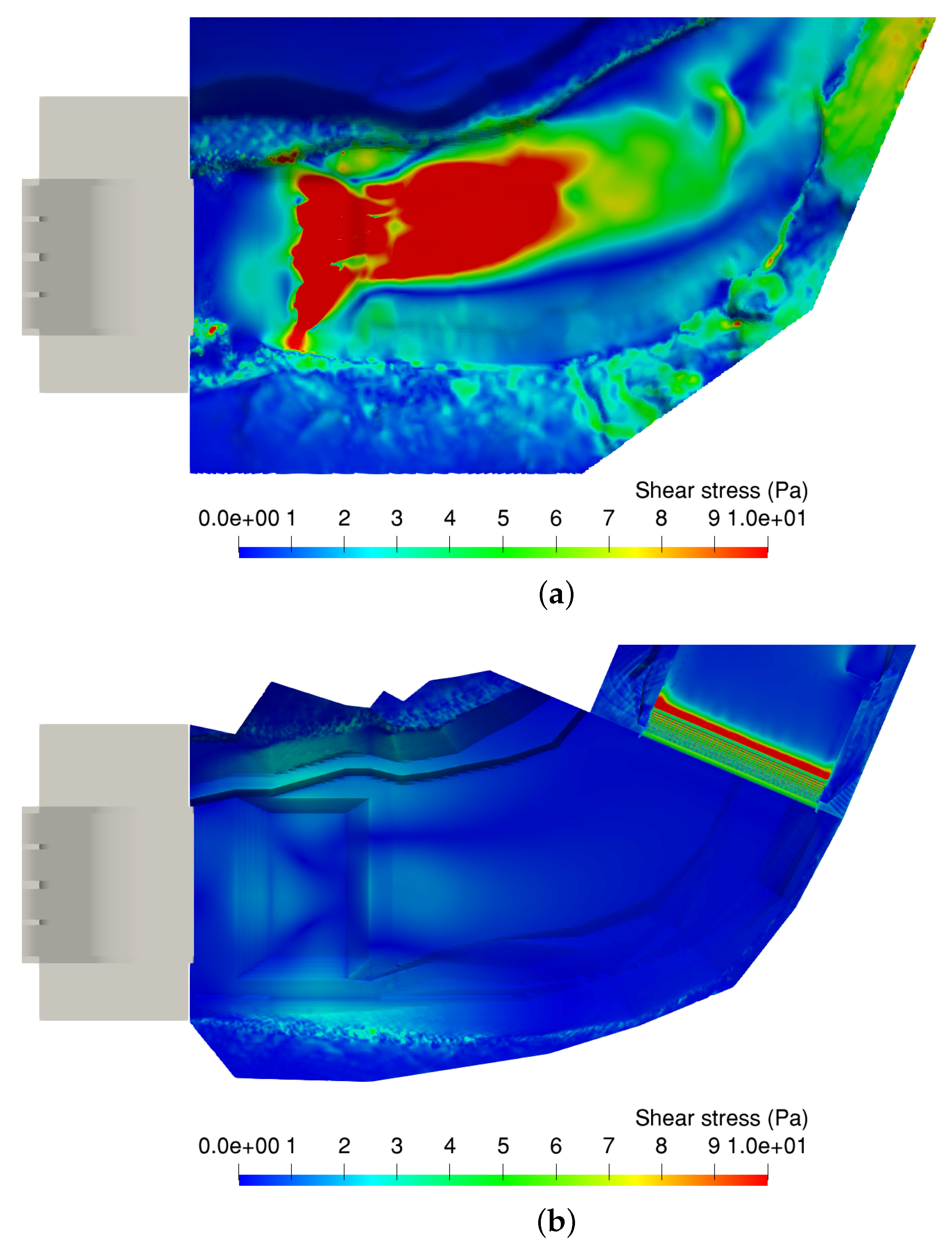
The flow structure near the impinging region is highlighted in Figure 13, where the flow speed is mapped on a vertical plane. Due to the absence of the secondary dam, the depth of the protective water cushion is very limited and the jet impinges on the bottom dissipation tank. Since flow velocities are extremely high, and the jet impacts on the bottom of the pool in absence of a deep water cushion, there is a high risk of long term erosion and protection measures have to be carefully designed in this area. Figure 14 shows how the shear stress on the dissipation tank and on the river bed increases and the high shear region extends further downstream. As displayed in Figure 15, in the comparison between the free surface in the two configurations, high velocities extend along the simulated domain. The numerical results give the relevant technical information needed for the design and evaluation of mitigation measures.
5. Discussion and Conclusions
A VOF-RANS model was applied to investigate the flood discharge from the spillway of the Sa Stria dam and its downstream routing in two different configurations. The implemented numerical model is able to reproduce, with a good accuracy, the mean variables of interest (water heights and pressures). Due to the inherent limitations of the RANS approach which, in general, can simulate accurately the mean variables but not the turbulent ones, numerical results are not adequate for pressure fluctuations computation in the present case. However, notwithstanding this limitation, the model gives a complete set of information on the hydraulics of the system, with an accuracy for the mean variables similar to a physical model at the same scale and with a greater amount of information over the whole simulation domain.
This allows us to properly investigate the dynamics of the overflow and dissipation processes, as well as the downstream flood routing. Thanks to the availability of laboratory validation measurements, the numerical study can hence provide adequate information to evaluate, with an appropriate uncertainty, different scenarios with respect to those already tested with the physical model as well as the proper framework to plan possible protection measures. Here we only simulated the hydrodynamic process that determines the erosion potential. It is worthwhile to mention that the possibility to apply three-dimensional numerical simulations to simulate also the scouring processes has been under study in literature [15].
Scale effects may affect reduced scale physical models simulated with Froude similarity. Specifically, aeration of the spillway jet reproduced at the model scale is less than in the prototype. The comparison of bottom mean pressures in the dissipation tank showed a good matching between numerical and physical modelling. This can be considered as an indirect proof of the correct reproduction of the spillway impact with the validation case. However, due to the scaling effect, at the prototype scale the impact point might be more upstream and a wider jet might be observed with respect to simulations (both laboratory and numerical ones). Indeed, being aware that full-scale CFD simulations allow overcoming the reduced-scale issues, here the choice was to deliberately reproduce the numerical model at the same scale of the physical one to assess whether a standard numerical model can usefully integrate a physical model. Indeed, in our work, the simulation of the set-up without the secondary dam in place at the prototype scale would have been inappropriate since validation was performed at the physical model scale. Moreover, due to the range of computed velocities, scaling issues are quite limited for the present simulation. According to [16], the trajectory deviation is meaningful for velocities around 40 m/s, while in case of velocities within 20 m/s scaling effects are negligible. An investigation of scale effects for labyrinth weir and a spillway modelling was performed by [17]. They evaluate the change in the results of numerical simulation at 1:25 scale and at the prototype scale, finding differences up to 15%, with scale effects reducing for larger flow rates.
From the modelling perspective, turbulent closures also play a major role as shown by the limited agreement of present results for the computed standard-deviation of pressure fluctuations when compared to measured data in the physical model. Indeed, the choice of the standard closure allowed meeting the object to integrate laboratory experiments with an adequate confidence on average variables. However, RANS results are sensitive to the choice of the turbulence closure; the most common models adopted in this field are standard , RNG , , SST [2]. According to [18] who compared the performances of these closure models for hydraulic jump simulation, the most accurate results were obtained with the RNG , although very fine meshes were necessary to ensure good performance, while the needed lower computational requirements without compromising accuracy excessively and being slightly better in reproducing the average water free surface. However, consensus on the best parametrisation has not been achieved yet in the scientific community. Indeed, additional insights from numerical and physical modelling are needed to develop CFD guidelines to apply RANS in this field, bearing in mind that the optimal solution depends on the target application and also to extent of the simulated domain.
On the other hand, despite other more advanced modelling techniques being available and successfully used in literature such as LArge Eddy Simulation (LES), Detached Eddy Simulation (DES) and Direct Numerical Simulation (DNS), their application is currently limited to a research context, mainly for simple free flow cases. These advanced methods are not suitable in the context of the dam design [2] and given the remarkable good agreement between present numerical results and measurements from the physical model, the RANS modelling still give a reasonably accurate and robust modelling framework from the engineering perspective.
As observed in [16], although models do not perfectly reproduce real phenomena, information inferred from models can be usefully adopted to find technical solutions, as long as model limitations are properly considered and their outcomes are adequately interpreted in an engineering perspective (for instance understanding whether and in which terms the modelled framework is conservative or not). With this in mind, the numerical approach here adopted can be useful to support the design and implementation of modifications to overflow structures and spillways of existing dams and climate change scenarios.
Author Contributions
Conceptualisation, M.G.B. and R.R.; methodology, M.G.B., R.R. and M.G.; software, M.G.B., R.R. and M.G.; validation, M.G.B. and R.R.; investigation, M.G.B. and R.R.; writing–original draft preparation, M.G.B., R.R. and M.G.; writing—review and editing, M.G.B., R.R. and M.G.; visualisation, M.G. and R.R.; supervision, M.G.B.; project administration, M.G.B.; funding acquisition, M.G.B. All authors have read and agree to the published version of the manuscript.
Funding
This research was partially funded by the Consorzio di Bonifica della Sardegna Meridionale-contract n. 0011749—CUP C29J04000010008-CIG 7266094A72.
Acknowledgments
The authors acknowledge the Consorzio di Bonifica della Sardegna Meridionale for providing the case study geometry and the laboratory dataset. In particular Egisto Mione and Alberto Carboni for the productive discussion.
Conflicts of Interest
The authors declare no conflict of interest.
References
- Olsen, N.R.B.; Kjellesvig, H.M. Three-dimensional numerical flow modelling for estimation of spillway capacity. J. Hydraul. Res. 1998, 36, 775–784. [Google Scholar] [CrossRef]
- Viti, N.; Valero, D.; Gualtieri, C. Numerical Simulation of Hydraulic Jumps. Part 2: Recent Results and Future Outlook. Water 2018, 11, 28. [Google Scholar] [CrossRef] [Green Version]
- Cook, C.B.; Richmond, M.C.; Serkowski, J.A. The Dalles Dam, Columbia River: Spillway Improvement CFD Study. Technical Report PNNL-14768, 969745; Pacific Northwest National Laboratory: Richland, WA, USA, 2006. [Google Scholar] [CrossRef] [Green Version]
- Ho, D.K.H.; Riddette, K.M. Application of computational fluid dynamics to evaluate hydraulic performance of spillways in australia. Austral. J. Civ. Eng. 2010, 6, 81–104. [Google Scholar] [CrossRef]
- Gadhe, V.; Patil, R.; Bhosekar, V.V. Performance assessment of upgraded spillway—Case study. ISH J. Hydraul. Eng. 2018, 1–9. [Google Scholar] [CrossRef]
- Demeke, G.K.; Asfaw, D.H.; Shiferaw, Y.S. 3D Hydrodynamic Modelling Enhances the Design of Tendaho Dam Spillway, Ethiopia. Water 2019, 11, 82. [Google Scholar] [CrossRef] [Green Version]
- Yang, J.; Andreasson, P.; Teng, P.; Xie, Q. The Past and Present of Discharge Capacity Modeling for Spillways—A Swedish Perspective. Fluids 2019, 4, 10. [Google Scholar] [CrossRef] [Green Version]
- Fluixá-Sanmartín, J.; Altarejos-García, L.; Morales-Torres, A.; Escuder-Bueno, I. Review article: Climate change impacts on dam safety. Nat. Haz. Earth Syst. Sci. 2018, 18, 2471–2488. [Google Scholar] [CrossRef] [Green Version]
- Aydin, M.C.; Isik, E.; Ulu, A.E. Numerical modeling of spillway aerators in high-head dams. Appl. Water Sci. 2020, 10, 1–9. [Google Scholar] [CrossRef] [Green Version]
- Chen, Q.; Dai, G.; Liu, H. Volume of Fluid Model for Turbulence Numerical Simulation of Stepped Spillway Overflow. J. Hydraul. Eng. 2002, 128, 683–688. [Google Scholar] [CrossRef]
- Rong, Y.; Zhang, T.; Peng, L.; Feng, P. Three-Dimensional Numerical Simulation of Dam Discharge and Flood Routing in Wudu Reservoir. Water 2019, 11, 2157. [Google Scholar] [CrossRef] [Green Version]
- Teng, P.; Yang, J. Modeling and Prototype Testing of Flows over Flip-Bucket Aerators. J. Hydraul. Eng. 2018, 144, 04018069. [Google Scholar] [CrossRef]
- Hirt, C.; Nichols, B. Volume of fluid (VOF) method for the dynamics of free boundaries. J. Comput. Phys. 1981, 39, 201–225. [Google Scholar] [CrossRef]
- van Leer, B. Towards the ultimate conservative difference scheme. V. A second-order sequel to Godunov’s method. J. Comput. Phys. 1979, 32, 101–136. [Google Scholar] [CrossRef]
- Castillo, L.G.; Carrillo, J.M. Comparison of methods to estimate the scour downstream of a ski jump. Int. J. Multiphase Flow 2017, 92, 171–180. [Google Scholar] [CrossRef]
- Novak, P.; Moffat, A.I.B.; Nalluri, C.; Narayanan, R. Hydraulic Structures: Fourth Edition; Taylor & Francis: Boca Raton, FL, USA, 2007; p. 725. [Google Scholar]
- Torres, C.; Borman, D.; Sleigh, A.; Neeve, D. Investigating Scale Effects of a Hydraulic Physical Model with 3D CFD. In Smart Dams and Reservoirs; ICE Publishing: Swansea, Scotland, 2018; pp. 89–101. [Google Scholar]
- Bayon-Barrachina, A.; Lopez-Jimenez, P.A. Numerical analysis of hydraulic jumps using OpenFOAM. J. Hydroinf. 2015, 17, 662–678. [Google Scholar] [CrossRef] [Green Version]
Figure 1.
Location of Sa Stria Dam, Sardinia (Italy). The planned position of the main and secondary dam, as well as the dissipation tank are shown in the construction site panel.
Figure 1.
Location of Sa Stria Dam, Sardinia (Italy). The planned position of the main and secondary dam, as well as the dissipation tank are shown in the construction site panel.

Figure 2.
Overview of the hex-dominant unstructured finite-volume grid employed in the simulations: (a) detail of the grid on the main spillway surface; (b) detail of the grid on the dissipation basin.
Figure 2.
Overview of the hex-dominant unstructured finite-volume grid employed in the simulations: (a) detail of the grid on the main spillway surface; (b) detail of the grid on the dissipation basin.

Figure 3.
Geometry model of the configuration with the downstream dam (the downstream dam is highlighted in red and the profile shown in the detail). The light blue transparent region denotes the simulation domain.
Figure 3.
Geometry model of the configuration with the downstream dam (the downstream dam is highlighted in red and the profile shown in the detail). The light blue transparent region denotes the simulation domain.

Figure 4.
Flow structure and velocity in the feeding tank at discharge flow rate of 300 .

Figure 5.
Initial condition of the water level for the configuration with the secondary dam. The two virtual hydrometers used to compare the water level with the experiments upstream of the secondary dam are shown in red.
Figure 5.
Initial condition of the water level for the configuration with the secondary dam. The two virtual hydrometers used to compare the water level with the experiments upstream of the secondary dam are shown in red.

Figure 6.
Comparison of predicted water level with measurements at the spillway crest.

Figure 7.
Locations (shown in red) for pressure measurements comparison with the experiments: (a) pressure probes at the bottom of the dissipation basin, (b) surfaces for average pressure calculation along the stair-step profile of the secondary dam (1, 3 and 5, horizontal surfaces; 2, 4 and 6, vertical surfaces). Note the labels of the pressure probes in the dissipation tank follows from that of the physical model.

Figure 8.
Visualisation of the overall water flow structure and velocity at discharge flow rate of 300 m with the rear dam in place.
Figure 8.
Visualisation of the overall water flow structure and velocity at discharge flow rate of 300 m with the rear dam in place.

Figure 9.
Local structure and contour maps of water flow speed in the impinging region of the jet at discharge flow rate of 300 m.
Figure 9.
Local structure and contour maps of water flow speed in the impinging region of the jet at discharge flow rate of 300 m.

Figure 10.
Local structure and speed of the water flow along the stair-step profile of the secondary dam.
Figure 10.
Local structure and speed of the water flow along the stair-step profile of the secondary dam.

Figure 11.
Geometry model of the configuration in the absence of the downstream dam. The light blue transparent region denotes the computational domain. The inflow section is highlighted in red.
Figure 11.
Geometry model of the configuration in the absence of the downstream dam. The light blue transparent region denotes the computational domain. The inflow section is highlighted in red.

Figure 12.
Visualisation of the overall water flow structure and velocity without the secondary dam at discharge flow rate of 300 m.
Figure 12.
Visualisation of the overall water flow structure and velocity without the secondary dam at discharge flow rate of 300 m.

Figure 13.
Structure and velocity field of the jet developing from the spillway and impinging on the dissipation basin without the secondary dam at discharge flow rate 300 m.
Figure 13.
Structure and velocity field of the jet developing from the spillway and impinging on the dissipation basin without the secondary dam at discharge flow rate 300 m.

Figure 14.
River bed shear stress for the simulations with (a) and without (b) the secondary dam.

Figure 15.
Free surface water structure and velocity comparison for the simulations with (a) and without (b) the secondary dam at discharge flow rate of 300 m.
Figure 15.
Free surface water structure and velocity comparison for the simulations with (a) and without (b) the secondary dam at discharge flow rate of 300 m.


Table 1.
Scaling parameters between the model and the prototype.
| Length: | = 1:40 | Speed: | = 1:6.325 |
| Time: | = 1:6.325 | Flow rate: | = 1:10119.3 |
Table 2.
Comparison between mean pressures computed in the physical and in the numerical model in the dissipation tank at discharge flow rate of 300 m. Corresponding standard deviations are displayed in brackets. Pressures are in meters of water column.
Table 2.
Comparison between mean pressures computed in the physical and in the numerical model in the dissipation tank at discharge flow rate of 300 m. Corresponding standard deviations are displayed in brackets. Pressures are in meters of water column.
| Probe 3 | Probe 8 | Probe 13 | Probe 18 | Probe 21 | |
|---|---|---|---|---|---|
| Physical model | 15.02 (0.15) | 15.10 (0.18) | 15.05 (007) | 15.02 (0.19) | 14.94 (0.17) |
| Numerical model | 14.83 (0.032) | 14.79 (0.029) | 14.81 (0.023) | 14.86 (0.018) | 14.92 (0.015) |
Table 3.
Comparison between mean pressures computed in the physical and in the numerical model in the secondary dam at discharge flow rate of 300 m. Pressures are in meters of water column.
Table 3.
Comparison between mean pressures computed in the physical and in the numerical model in the secondary dam at discharge flow rate of 300 m. Pressures are in meters of water column.
| Sensor 1 | Sensor 2 | Sensor 3 | Sensor 4 | Sensor 5 | Sensor 6 | |
|---|---|---|---|---|---|---|
| Physical model | 0.76 | −0.08 | 0.98 | 0.34 | 1.46 | 0.10 |
| Numerical model | 0.64 | 0.27 | 0.82 | 0.32 | 1.13 | 0.11 |
© 2020 by the authors. Licensee MDPI, Basel, Switzerland. This article is an open access article distributed under the terms and conditions of the Creative Commons Attribution (CC BY) license (http://creativecommons.org/licenses/by/4.0/).
Share and Cite
MDPI and ACS Style
Badas, M.G.; Rossi, R.; Garau, M. May a Standard VOF Numerical Simulation Adequately Complete Spillway Laboratory Measurements in an Operational Context? The Case of Sa Stria Dam. Water 2020, 12, 1606. https://doi.org/10.3390/w12061606
AMA Style
Badas MG, Rossi R, Garau M. May a Standard VOF Numerical Simulation Adequately Complete Spillway Laboratory Measurements in an Operational Context? The Case of Sa Stria Dam. Water. 2020; 12(6):1606. https://doi.org/10.3390/w12061606
Chicago/Turabian StyleBadas, Maria Grazia, Riccardo Rossi, and Michela Garau. 2020. "May a Standard VOF Numerical Simulation Adequately Complete Spillway Laboratory Measurements in an Operational Context? The Case of Sa Stria Dam" Water 12, no. 6: 1606. https://doi.org/10.3390/w12061606
Note that from the first issue of 2016, this journal uses article numbers instead of page numbers. See further details here.