Black Hole as a Quantum Field Configuration

1
Department of Physics, Kyoto University, Kitashirakawa, Kyoto 606-8502, Japan
2
iTHEMS, RIKEN, Wako, Saitama 351-0198, Japan
*
Author to whom correspondence should be addressed.
Universe 2020, 6(6), 77; https://doi.org/10.3390/universe6060077
Submission received: 23 March 2020
/
Revised: 30 May 2020
/
Accepted: 30 May 2020
/
Published: 4 June 2020
(This article belongs to the Section Gravitation)
Abstract
:We describe 4D evaporating black holes as quantum field configurations by solving the semi-classical Einstein equation and quantum matter fields in a self-consistent manner. As the matter fields, we consider N massless free scalar fields (N is large). We find a spherically symmetric self-consistent solution of the metric and the state . Here, is locally geometry, and provides , where is the ground state of the matter fields in the metric and consists of the excitation of s-waves that describe the collapsing matter and Hawking radiation with the ingoing negative energy flow. This object is supported by a large tangential pressure due to the vacuum fluctuation of the bound modes with large angular momenta . This describes the interior of the black hole when the back reaction of the evaporation is taken into account. In this picture, the black hole is a compact object with a surface (instead of horizon) that looks like a conventional black hole from the outside and eventually evaporates without a singularity. If we count the number of configurations that satisfy the self-consistent equation, we reproduce the area law of the entropy. This tells that the information is carried by the s-waves inside the black hole. also describes the process that the negative ingoing energy flow created with Hawking radiation is superposed on the collapsing matter to decrease the total energy while the total energy density remains positive. Finally, as a special case, we consider conformal matter fields and show that the interior metric is determined by the matter content of the theory, which leads to a new constraint to the matter contents for the black hole to evaporate.
1. Introduction
In quantum theory, black holes evaporate [1]. This property may change the definition of black holes from the classical one. It should be determined by quantum dynamics of matter and spacetime. By collapse of a star, an object should be formed and evaporate in a finite time. The Penrose diagram of the space-time should have the same topology structure as the Minkowski space-time, where there is no event horizon or singularity but may be a trapping horizon. Such an object should be the black hole. This view is an accepted consensus in the context of quantum theory [2,3,4,5,6,7,8,9,10,11,12,13,14,15,16,17,18,19,20,21,22,23,24,25,26,27]1. In this paper, we consider this problem in field theory and find a picture of the black hole.
First, we briefly describe our basic idea. (In Section 2, we will provide a more detailed picture). Suppose that we throw a test spherical shell or particle into an evaporating spherically symmetric black hole. If the black hole evaporates completely in a finite time without any singular phenomenon, the particle should come back after evaporation. Let’s take a closer look at this process. As the particle comes close to the Schwarzschild radius of the black hole, it becomes ultra-relativistic and behaves like a massless particle [40]. Then, if we take into account the time-dependence of the metric due to the back reaction of evaporation, the particle does not enter the time-dependent Schwarzschild radius but moves along an ingoing null line just outside it [9], which will be explicitly shown below Equation (6). After the black hole evaporates, the particle returns to the outside.
Here, one might think that this view is strange. In a conventional intuition, a collapsing matter should enter soon the slowly decreasing Schwarzschild radius because a typical time scale of evaporation is much larger than that of collapse . Here, is the Schwarzschild radius of the black hole with mass M, is the Planck length, t is the time coordinate at infinity, and is that of a comoving observer along the collapsing matter. However, it doesn’t make sense to compare these two time scales, which are measured by different clocks. In the above argument, we have considered the both time evolutions of the spacetime and particle in a common time. We will see (around Equation (7)) that the back reaction of the evaporation plays a non-negligible role in determining the motion of the particle at a Planck length distance from the Schwarzschild radius.
Now, let us consider a process in which a spherical matter collapses to form a black hole. We can focus on the motion of each of the spherical layers that compose the matter because of the spherical symmetry. As a layer approaches the Schwarzschild radius that corresponds to the energy of itself and the matter inside it, it moves at the speed of light. At the same time, the time-dependent spacetime (without a horizon structure) causes particle creation [41,42] (which is so-called pre-Hawking radiation [9,16,43,44]), and the energy begins to decrease2. Indeed, we will show in Section 2 that this pre-Hawking radiation has the same magnitude as the usual Hawking radiation. Then, applying the above result about the motion of the particle, we can see that the layer keeps falling just outside the time-dependent Schwarzschild radius. As this occurs for all the layers, the entire of the collapsing matter just shrinks to form a compact object, which is filled with the matter and radiation. Here, it should be noted that a strong tangential pressure occurs inside to stabilize the object against the gravitational force [9]. The pressure is consistent with 4D Weyl anomaly and so strong that the interior is anisotropic locally (that is, the interior is not a fluid) and the dominant energy condition breaks down [14,16,24]. Therefore, this object doesn’t contradict Buchdahl’s limit [45]. (We will explain the origin of the pressure later).
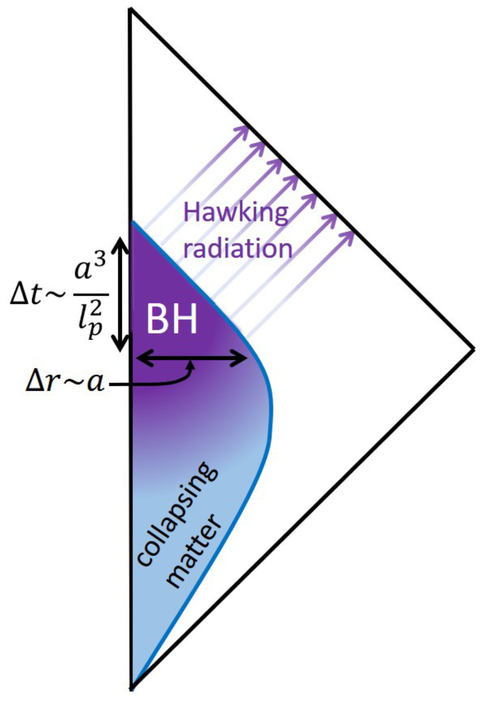
The object has (instead of horizon) a null surface just outside the Schwarzschild radius and looks like the classical black hole from the outside, whose spatial size is . Here, the surface is the boundary between the interior dense region and the exterior dilute region. Eventually, it evaporates in a time .3 This object should be the black hole in quantum theory [9,14,16,24]. As we will see, there is no singularity. (No trans-Planckian quantity appears if the theory has many degrees of freedom of matter fields). Therefore, the Penrose diagram is given by Figure 1, and the spacetime region of and corresponds to the black hole. In this paper, we show that this story can be realized in field theory.
Strategy and Result
The above idea has been checked partially by a simple model [9], a phenomenological discussion [14] and the use of conformal matter fields [24]. It also holds for charged black holes and slowly rotating black holes [16]. Furthermore, by a thermodynamical discussion, the entropy density inside the object is evaluated and integrated over the volume to reproduce the area law [16]. Therefore, it seems that this picture is plausible and works universally for various black holes.
However, there still remain several questions about this picture. What is the self-consistent state ? What configurations do the matter fields take inside? How is the large tangential pressure produced inside? Can we reproduce the entropy area law by counting microscopic states of fields? How does the energy of the collapsing matter decrease? These are crucial for understanding what the black hole is and how the information of the matter comes back after evaporation.
In this paper, to answer these questions, we analyze time evolution of a 4D spherical collapsing matter by solving the semi-classical Einstein equation
in a self-consistent manner, and we find the metric and state which represent the interior of the black hole. Here, we treat gravity as a classical metric while we describe the matter as N massless free quantum scalar fields. is the renormalized expectation value of the energy-momentum tensor operator in that contains the contribution from both the collapsing matter and the Hawking radiation.
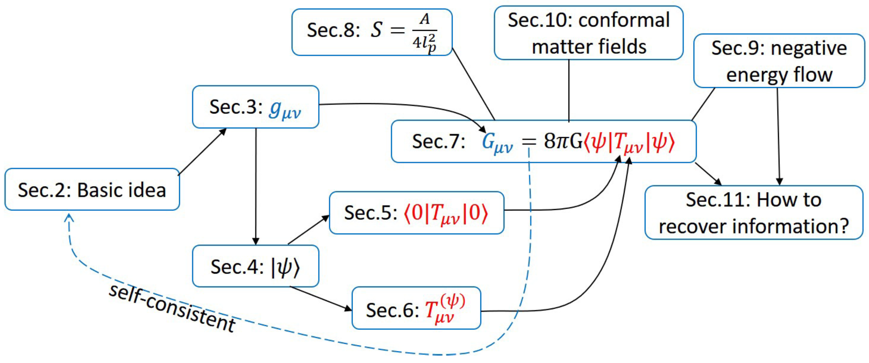
We explain our self-consistent strategy and the results. The flow chart of Figure 2 represents the composition of this paper.
In Section 2, we first explain our basic idea in a more concrete manner by using a simple model. We also show how the pre-Hawking radiation occurs in the time-evolution of the system. In Section 3, we employ and generalize the model and construct a candidate metric . In particular, the interior metric is shown to be static as a result of dynamics. It can be expressed as
We write down two functions in terms of two phenomenological functions: one is the intensity of Hawking radiation and the other is a function that provides the ratio between the radial pressure and energy density. We also show that this metric is locally geometry.
We are interested in the black holes most likely to be formed in gravitational collapse. As shown in Section 6, the statistical fluctuation of the mass is evaluated as , where is the Planck mass. Therefore, from a macroscopic perspective, all black holes with mass are the same. We consider the set of states that represent the interior of such statistically identified black holes.
In Section 4, we examine the potential energy of the partial waves of the scalar fields in the interior metric. Modes with angular momenta are trapped inside, and they emerge in the collapsing process even if they don’t exist at the beginning. We show that, if such bound modes are excited, the energy increases by more than , which means that the number of excited bound modes is at most order of in the set . Therefore, those modes can be regarded as the ground state because is negligible compared to the number of total modes (which is shown in Section 6). On the other hand, s-wave modes can enter and exit the black hole and represent the collapsing matter and Hawking radiation. Thus, the state provides
where is the ground state in the interior metric, and is the contribution from the excitations of the s-waves.
In Section 5, we evaluate . We first solve the equation of motion of the scalar fields in the interior metric. We calculate the regularized energy-momentum tensor in the dimensional regularization. Then, we renormalize the divergences and obtain the finite expectation value, . This contains contributions from the finite renormalization terms , which correspond to the renormalized coupling constants of and in the action, respectively.
In Section 6, we combine Bekenstein’s discussion of black-hole entropy [46] and our picture of the interior of the black hole to infer the form of , which is fixed by a parameter .
In Section 7, we solve Equation (1) by using the ingredients obtained so far: , , and . We determine the self-consistent values of for a certain class of the finite renormalization terms . We then check the various consistency. In particular, we see that there is no singularity, and that the vacuum fluctuation of the bound modes with creates the large tangential pressure .
In Section 8, we consider the stationary black hole which has grown up adiabatically in the heat bath. We count the number of the states of the s-waves inside the black hole to evaluate the entropy, reproducing the area law. This implies that the information is carried by the s-waves.
In Section 9, to understand the mechanism by which the energy of the collapsing matter decreases, we assume a s-wave model for simplicity to describe the outermost region of the black hole and study the time evolution of quantum fields. We see that describes the process that the negative ingoing energy flow created with Hawking radiation is superposed on the collapsing matter to decrease the total energy while the total energy density remains positive.
Thus, three independently conserved energy-momenta appear in this solution: that of the bound modes of the vacuum , that of the collapsing matter, and that of the pair of the Hawking radiation and negative energy flow, where the last two contribute to . These three form the self-consistent configuration of the black hole.
In Section 10, as a special case, we consider conformal matter fields and show that the parameters are determined by the matter content of the theory. Interestingly, the consistency of provides a condition to the matter content. For example, the Standard Model with a right-handed neutrino satisfies the constraint but a model without it doesn’t. Therefore, this can be regarded as a new constraint (like the weak-gravity conjecture [47,48]) that is required in order for the black hole to evaporate.
In Section 11, we conclude and discuss future directions. In particular, we discuss how the information comes back after evaporation if there are interactions between the collapsing matter, Hawking radiation, and negative energy flow.
In Appendices, we give the derivation of various key equations. In particular, we explain the difference between our pre-Hawking radiation and the usual Hawking radiation in Appendix C.
2. Basic Idea
We explain our basic idea of the black hole more precisely [9,14,16,24], which makes the motivation of this paper clearer. The discussion is composed of three steps. In step1, we examine the motion of a thin shell (with an infinitely small mass) near an evaporating black hole and anticipate what will be formed as a result of the time evolution of a spherical collapsing matter. In step2, we study the time evolution of the pre-Hawking radiation induced by the shell, including the effect of a small finite mass of the shell and the radiation. In step3, we construct a simple model (multi-shell model) to realize the prediction given in step1, and show that the pre-Hawking radiation has the same magnitude as that of the usual Hawking radiation. We also discuss a surface pressure on the shell induced by the pre-Hawking radiation.
2.1. Step1: Motion of a Shell Near the Evaporating Black Hole
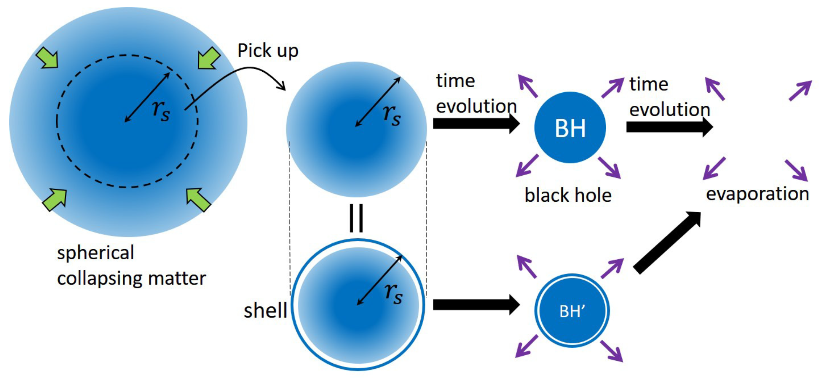
Imagine that a spherical collapsing matter with a continuous distribution starts to collapse (see the left of Figure 3).
We pick up a part of it with a radius . When the radius comes close to the Schwarzschild radius of the mass inside it, the entire of the part behaves light-like. Then, we can discuss the time evolution of the part without considering the outside because the outside matter does not come in and has no influence to the inside due to the spherical symmetry (see the center of the upper in Figure 3). We suppose that the part becomes a black hole and evaporates eventually (see the right of the upper in Figure 3). Now, we consider the outermost part of the collapsing matter as a spherical thin shell (which is located at ) with an infinitely small energy (see the center of the lower in Figure 3). Focusing on the motion of the shell, it will approach the evaporating black hole consisting of the rest (see the right of the lower in Figure 3). (Note again that the rest part is not affected by the shell and becomes the evaporating black hole). As we show in the following, the black hole evaporates to disappear before the shell catches up with “the horizon", and thus the shell will never enter “the horizon”.
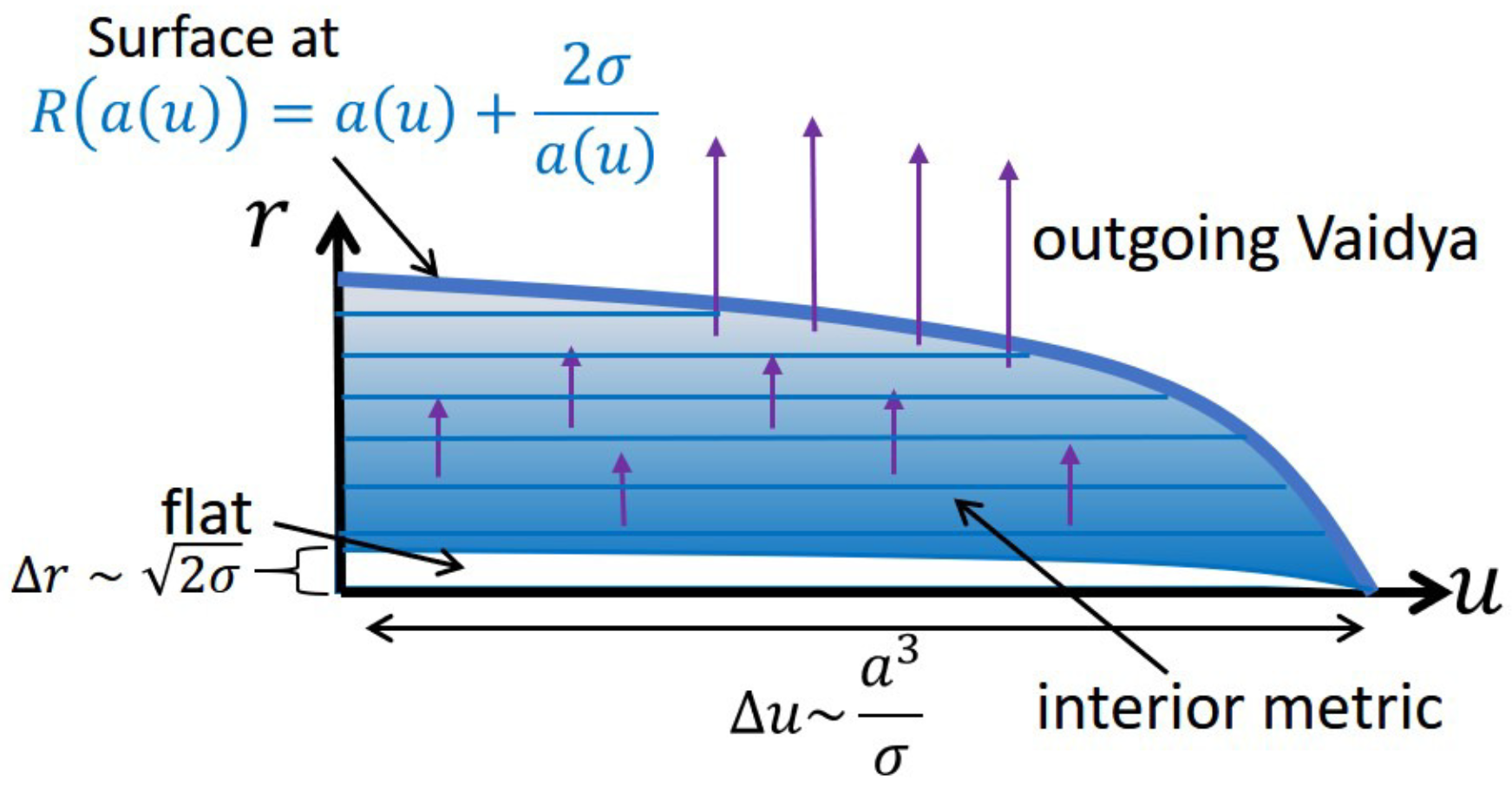
Because of the spherical symmetry, the gravitational field that the shell feels is determined by the energy of itself and the matter inside it, no matter what is outside the shell. Therefore, the metric which determines the motion of the shell near the black hole is given approximately by the outgoing Vaidya metric [49]
where u is the null coordinate that represents an outgoing radial null geodesic as const. is the energy inside the shell at time u (including the energy of the shell itself)4. The Einstein tensor has only and satisfies , and therefore this metric can represent the outgoing null energy flow with total flux 5 6. Thus, we assume that decreases according to the Stefan–Boltzmann law of Hawking temperature :
Here, is the intensity of the Hawking radiation, which is determined by dynamics of the theory. In general, it takes the form of , where k is an constant.
Suppose that the shell consists of many particles. If a particle of them comes close to , the motion is governed by the equation for an ingoing radial null geodesic,
no matter what mass and angular momentum the particle has7. Here, is the radial coordinate of the particle (or the shell).
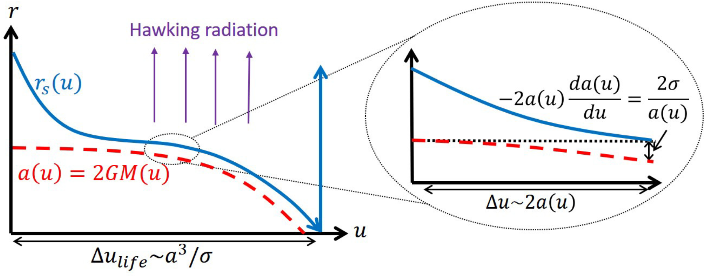
At this point, we can see a general property of Equation (6): Once a particle starts from a position outside , the particle comes close to but does not pass it. Therefore, if decreases to zero in a finite time, the particle will reach the center in a finite time and return to . See the left of Figure 4.
Note that the radius becomes zero in a finite time (), and the time coordinate u describes the outside spacetime region globally.
Here, we stress that we have no coordinate singularity in this analysis. First, we note that the Vaidya metric (4) with Equation (5) is the metric around the trajectory of the particles that composes the outermost shell of the collapsing matter (remember the center of the lower in Figure 3). It seems that the metric has coordinate singularity at . However, because is assumed to become zero in a finite time, the particle moves according to Equation (6) and stays always outside . In particular, when becomes zero, is still positive. After that, propagates in the flat space and reaches in a finite time8. Actually, as we will see in Equation (10), is always apart from at least by the proper length , which is physically long if N is large (see the discussion below Equation (11)). Of course, at the final stage of the evaporation, which exceeds the semi-classical approximation, a curvature singularity may occur. However, the black hole at that moment has only a few of Planck mass and should be considered as a stringy object (see also footnote 3). (We can show that, even if we used the metric (4) to describe such a final stage, and would never become zero at the same time. See Appendix B). Thus, the particle keeps moving outside without coordinate singularity. Finally, we emphasize that, when we consider a particle that starts to fall before the shell we have focused, the metric around the trajectory of the particle is not the Vaidya metric with . Rather, it is given by another Vaidya metric with the Schwarzschild radius of the energy of the matter inside the shell to which the particle belongs. See the following discussion and Section 2.3.
Let us examine more specifically where will approach when evolves according to Equation (5). We are interested in the difference , which is much smaller than , . Then, in the denominator of Equation (6) can be replaced with approximately, and Equation (6) becomes
The first term in the r.h.s. is negative, which is the effect of collapse, and the second one is positive due to Equation (5), which is the effect of evaporation. The second term is negligible when , but it becomes comparable to the first term when the particle is so close to that . Then, the both terms are balanced so that the r.h.s of Equation (7) vanishes, and we have . This means that any particle moves asymptotically as
and so does the shell. By solving Equation (7) explicitly, we can check that this approach occurs exponentially in the time scale (see Appendix A).
This behavior can be understood as follows. See the right side of Figure 4. The particle approaches the radius in the time . During this time, the radius itself is slowly shrinking as Equation (5). Therefore, cannot catch up with completely and is always separate from by .
Thus, considering the time evolution of both the particle and spacetime together, we have reached the conclusion that any particle never enters “the horizon”. Therefore, the shell (consisting of the particles) will move according to Equation (8) just outside “the horizon”.
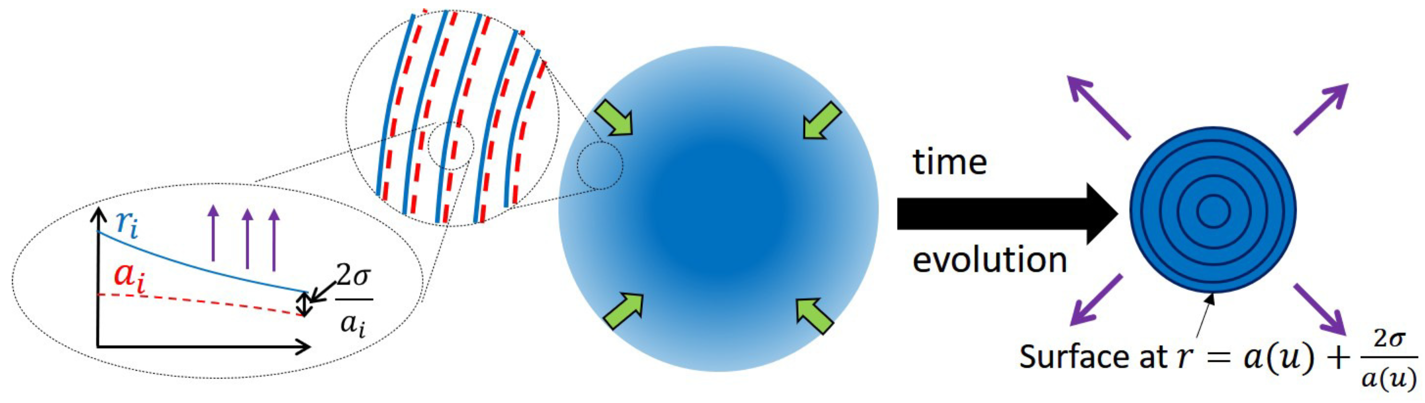
Because the above argument holds for any radius (recall the center of the upper in Figure 3), we can imagine that the entire matter consists of many spherical thin shells. See Figure 5.
That is, when we focus on any part of it with radius and mass , the shell (particle) at moves asymptotically as if the inner part evaporates as (see the left of Figure 5). Here, is the local time just outside the shell. If this happens in the whole part of the matter, it implies that many shells pile up and form a dense object with the total mass M (see the right of Figure 5). The object has, instead of a horizon, a surface as the boundary between the high-density interior and the low-density exterior at
where the total radius decreases as Equation (5). This object looks like a conventional black hole from the outside because , while it is not vacuum and has an internal structure. Eventually, it evaporates in , and the Penrose diagram should be represented as in Figure 1. This should be the black hole in quantum theory. In the following two steps, we will gradually describe this picture precisely.
Before going to the next step, one might wonder here if the above idea can be realized in field theory or not. To see this point simply, we examine the distance more because it is the typical length scale in this picture. The proper length is evaluated as 9
where Equations (4) and (9) have been used. We here assume that N is large but finite, for example, :
Then, is larger than , and is sufficiently long in order for the effective local field theory to be valid. In particular, the position of the surface (9) is meaningful physically. A way to show the validity of the field theory more precisely is to construct a concrete solution by solving Equation (1) and confirm its self-consistency. From Section 3, we will do it.
2.2. Step2: Pre-Hawking Radiation
In the step1, we have neglected the effect of the mass of the shell and considered only the Hawking radiation from the black hole inside the shell. In this step, we will take into account the effect of the mass and a pre-Hawking radiation.
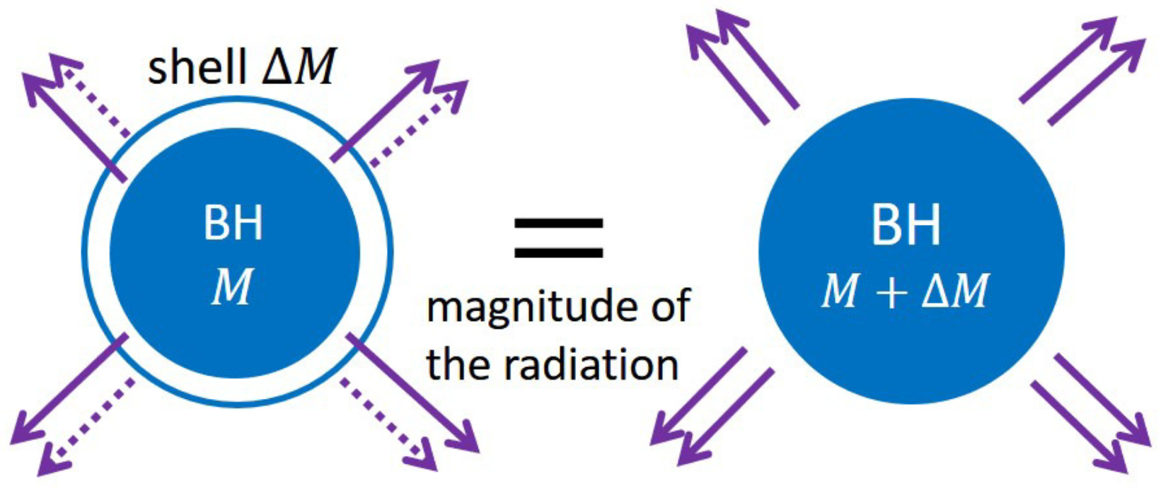
Suppose that we add a spherical thin null shell with a small but finite energy to the black hole with mass M evaporating as Equation (5) 10. From now, we will show that a pre-Hawking radiation is induced by this shell so that the total magnitude of the pre-Hawking radiation and the Hawking radiation from the black hole is equal to that of the Hawking radiation from a larger black hole of mass (up to corrections). See Figure 6.
Therefore, the total system of the black hole and the shell behaves like a larger black hole. (This provides a more precise description of the right of the lower in Figure 3).
2.2.1. Setup
Although we will start a 4D complete analysis from Section 3, here for simplicity we consider only s-waves of N massless scalar fields. For example, by using the conservation law with 2D Weyl anomaly [41,50,51,53], we can evaluate the outgoing flux from the center black hole as
Comparing this to Equation (5), we see the intensity of s-wave Hawking radiation:
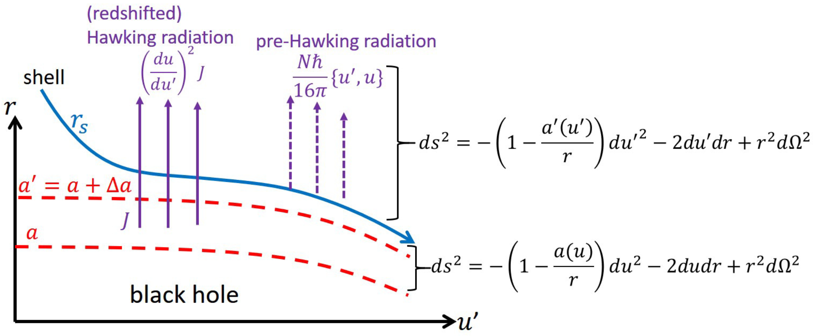
We are now interested in the situation where the shell comes to the black hole as in Figure 7.
Because of the spherical symmetry, the region between the black hole and the shell is still described by the metric (4) with Equation (5) of the intensity (13) 11, while the region above the shell is expressed by another Vaidya metric
Here, is the Schwarzschild radius of the total mass, and the time is different from u due to the mass of the shell .
The evolution equation of is given by the energy conservation, , where is the total flux coming out of the total system. In general, particles are created in a time-dependent spacetime of a collapsing matter. It is well-known that we can formulate the s-wave approximated energy flux of the particles as [53,54,55]
Here, U is the outgoing null time of the flat spacetime before the collapse, and is the Schwarzian derivative for . (See above Equation (33) for a more explanation). Using a formula [56]
and applying Equations (12) and (13), we have
This has a physical interpretation. See Figure 7. The first term represents the energy flux from the black hole (12), that is redshifted due to the mass of the shell, and the second one corresponds to the radiation induced by the shell. We call this term pre-Hawking radiation because any horizon structure is not relevant to . Thus, the total of the redshifted Hawking radiation and the pre-Hawking radiation determines time evolution of the energy of the total system:
which is nothing but the -component of the semi-classical Einstein equation.
To relate u and each other, we use a fact that the trajectory of the shell, , is null from both sides of the shell to get the connection conditions:12
This is equivalent to Equation (6) and
2.2.2. Time Evolution of the Pre-Hawking Radiation
We examine how the pre-Hawking radiation occurs by solving directly the coupled time-evolution Equations (18) and (21). Here, we consider linearized equations for .
In the linear order of , from the evaluation (21), we have
where the dot stands for the u derivative (e.g., ). Note that once the quantity is linear in , we no longer need to distinguish u derivative from derivative because of Equation (21). In order to get Equation (22), we have used an identity for the Schwarzian derivative
and the fact that and , which will be checked in a self-consist manner below.
As mentioned above, the derivative in the l.h.s. can be replaced to u derivative, and we reach
This determines the time evolution of and how the pre-Hawking radiation is emitted.
Let us solve Equation (25) in the time scale , where hardly changes because of Equation (5). Putting the ansatz into Equation (25), we have
that is, . means that the energy of the shell increases exponentially in time, which is not accepted physically. Here, one might wonder why such an unphysical solution appears. The reason is that Equation (18) is a higher derivative equation describing the back reaction of the radiation to be created in the time evolution. A similar problem occurs in “Lorentz friction” (a recoil force on an accelerating charged particle caused by electromagnetic radiation emitted by the particle), where one must choose a physical solution by hand [40]. In the present case, therefore, we select as the physical solution
This indicates that, as the pre-Hawking radiation is emitted, the energy of the shell decreases exponentially in the time scale 13. In particular, this solution satisfies
This agrees with up to , which shows that Figure 6 holds as a result of the time evolution. (In the next step, we will show including the correction of ). It should be noted that, on the third line of Equation (29), the amount of the Hawking radiation reduced by the redshift is compensated by the pre-Hawking radiation14. Therefore, the pre-Hawking radiation plays an essential role in the evaluation (29).
2.3. Step3: A Multi-Shell Model
We have seen so far that the statement of Figure 6 works up to corrections for any part of the collapsing matter. Therefore, we can imagine that the collapsing matter consisting of many shells shrinks emitting the pre-Hawing radiation from each shell in the time evolution. In this last step, we will construct a dynamical model representing the situation and show under the s-wave approximation that the pre-Hawking radiation is emitted with exactly as the same magnitude as the usual Hawking radiation. Then, we see that a surface pressure is induced on each shell by the pre-Hawking radiation and discuss its role in the time evolution.
2.3.1. Setup
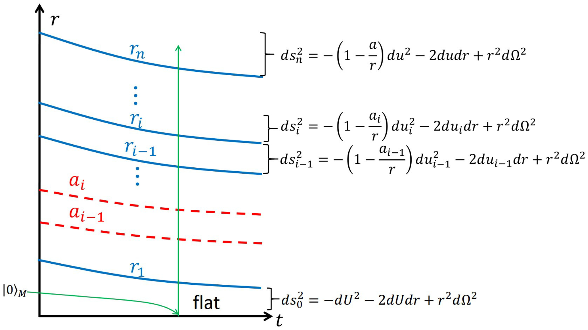
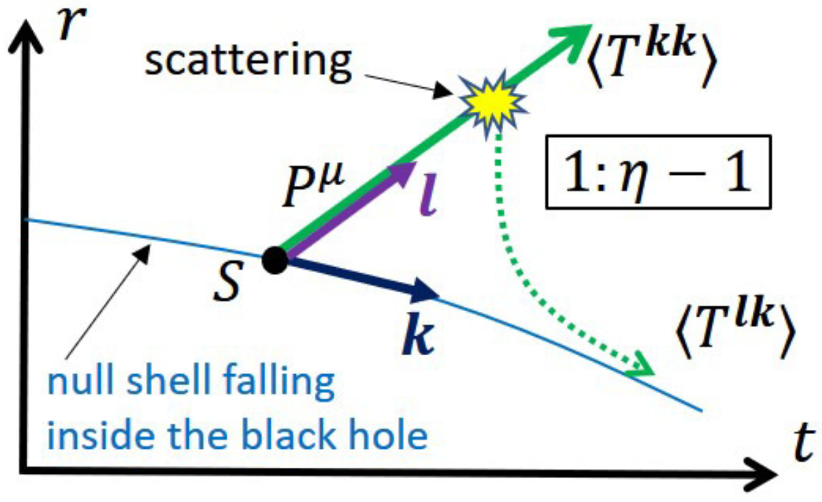
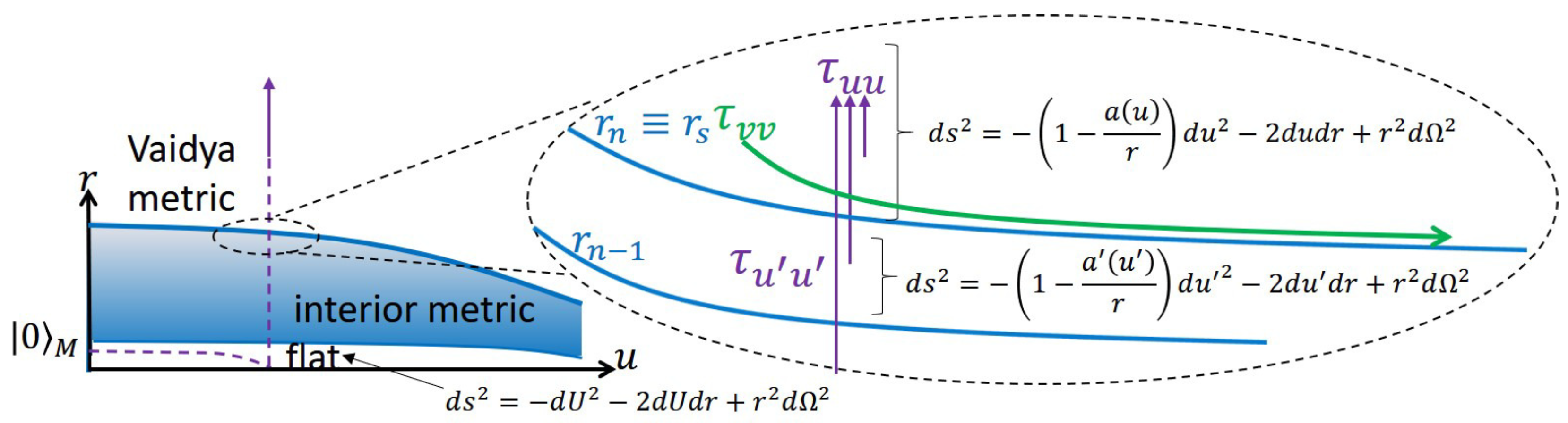
We consider a spherical collapsing matter consisting of n spherical thin null shells. See Figure 8, where represents the position of the i-th shell.
Here, physically, some part of the radiation emitted from a shell can be scattered by the other shells or the gravitational potential, but we neglect the effect for simplicity. (We will introduce it in Section 3.2.1). Then, because of spherical symmetry, for , the region just outside the i-th shell can be described by the outgoing Vaidya metric:
Here, is the local time, , and is the energy inside the i-th shell (including the contribution from the shell itself). For , is the time coordinate at infinity, and , where M is the total mass. That is, the outside is given by the metric (4), but we do not assume Equation (5). On the other hand, the center, which is below the 1-st shell, is the flat spacetime,
because of the spherical symmetry. Therefore, we can regard that
To set the time evolution equations of , we consider how particle creation occurs in this time-dependent spacetime [1]. Suppose that the quantum fields start in the Minkowski vacuum state from a distance. They come to and pass the center as the green arrow in Figure 8. Then, they will propagate through the matter and be excited by the curve metric to create particles, which corresponds to the pre-Hawking radiation. For example, by solving the field equation in the eikonal approximation and using the point-splitting regularization [9,16], we can evaluate the total outgoing energy flux observed just above the i-th shell as
for . Therefore, we have for each i
To complete the setup, we need to connect time coordinates, . Following the idea used to get the conditions (19), we have the connection conditions at :
This is equivalent to
and
2.3.2. Check of the Pre-Hawking Radiation
In order to solve the coupled Equations (34) and (35), let us take the continuum limit by . In particular, we focus on a configuration in which the following ansatz holds:15
These can be justified by the result of step 2: From the outside of the i-th shell, the system consisting of the shell and its inside behaves like the ordinary evaporating black hole as in Equation (5), and the shell comes close to the asymptotic position as in Equation (8).
In the following, we show that the ansatz (38) and (39) gives a solution to the coupled equations to be solved, (34), (36), and (37). First of all, the ansatz (39) is nothing but the asymptotic solution of Equation (36) under the assumption (38). As we will see below, there exists a C that makes Equations (34) and (37) be satisfied.
Here, on the second line, we have used Equation (37); on the third line, we have used the ansatz (39) and assumed ; and, on the last line, we have approximated . These approximations become exact in the continuum limit. Then, with the condition (32), we obtain
Next, we consider the time evolution Equation (34). We first note that from the definitions of the Schwarzian derivative and (see Equation (40)), we have
On the other hand, from Equations (42) and (38), we have
Therefore, we have
where the higher terms in have been neglected for . Using this, Equations (34), and (38), we find . That is, the solution tells that the system inside (including) each shell evaporates emitting the pre-Hawking radiation with the same magnitude as the usual Hawking radiation:
Note again that this is not an assumption but the result of solving the semi-classical Einstein equation in the s-wave approximation [9,16]. Thus, we have seen in the s-wave approximation that the collapsing matter becomes a dense object with the surface (9) and evaporates as in Figure 5. The pre-Hawking radiation is emitted from each shell, and the sum of them comes out of the surface of the object just like the usual Hawking radiation. In the following, we will use the term “Hawking radiation” to mean the pre-Hawking radiation 16. (In Appendix C, we compare this pre-Hawking radiation to the usual Hawking radiation [1]).
Here, one might wonder how the Planck-like distribution with the Hawking temperature is obtained in this pre-Hawking radiation. Suppose that we want to evaluate the distribution of the particles created around a time . Because changes slowly as Equation (46), we can approximate it as (where ), which leads to . Using this, Equations (40) and (42) with , we have
Note that U is the affine parameter for outgoing null modes in the initial flat space, and u is that in the asymptotically flat region of the spacetime after the formation of the black hole. In general, such an exponential relation between the two affine parameters plays an essential role in obtaining the Planck-like distribution of the Hawking temperature [43,44]. In fact, the relation (47) leads to the Planck-like distribution of the time-dependent Hawking temperature [9,16] 17
Therefore, it is possible to discuss black-hole thermodynamics by using the pre-Hawking radiation (without any horizon structure) and consider the entropy (see Section 8).
2.3.3. Surface Pressure Induced by the Pre-Hawking Radiation
We check the junction condition along the trajectory of each shell and study why the matter does not collapse. When two different metrics are connected at a null hypersurface, a surface energy-momentum tensor exists on it generically. By using the Barrabes–Israel formalism [57,58], we can calculate the surface energy density and the surface pressure on the i-th shell as (see Appendix F of [16] for the derivation)
Naturally, expresses the energy density of the shell with energy and area . Using Equations (34) and (37) and then applying the formula (16) to , we can express as
which shows through Equation (17) that the pressure is induced by the pre-Hawking radiation .
Let us evaluate . We start with the expression (49). Using Equations (39) with and (46) and performing a similar calculation to the evaluation (29), we obtain
for . Therefore, the pressure is positive and strong (even for ). This means that, as the shell contracts, the pressure works to resist the gravitational force while the pre-Hawking radiation is dissipated.
We can understand the origin of this pressure from a 4D field-theoretic point of view. Indeed, the pressure appears naturally from conservation law and 4D Weyl anomaly [24]. In the following sections, we will calculate directly the expectation value of the energy-momentum tensor and show that the vacuum fluctuation of the bound modes with creates the pressure.
3. Construction of the Candidate Metric
From now, we start a full 4D self-consistent discussion, and show that the basic idea works as a solution of the Einstein Equation (1). In the present and following sections (except for Section 9), we do not employ the s-wave approximation used in the previous section, but we consider the full 4D dynamics of quantum fields.
In this section, we use and generalize the multi-shell model in the previous section and construct a candidate metric for the interior [9,14,16,24]. Note that at this stage we do not mind if the metric is the solution of the Equation (1) or not. In Section 7, we will show that indeed it is.
3.1. The Interior Metric
We use the multi-shell model of Figure 8 and construct a candidate metric for the interior of the object. To do that, we suppose again that in the continuum limit the ansatz
hold for an intensity . Then, we can use these and the condition (37) to obtain (like the calculation (41))
Note that in the previous section we have used the s-wave approximated Einstein Equation (34) to obtain in Equation (46), but we are now trying to use the full 4D Einstein equation to identify the self-consistent value of (see Section 7).
Now, the metric at a spacetime point inside the object is obtained by considering the shell that passes the point and evaluating the metric (30). We have at
where Equations (52) and (53) have been used. From these, we can obtain the metric
Note that this is static although each shell is emitting the pre-Hawking radiation and shrinking physically.
Thus, our candidate metric for the evaporating black hole is given by [9]
under the assumption that the scattering effects are neglected. See Figure 9.
This metric is continuous at the null surface located at , where the total Schwarzschild radius decreases as Equation (5). Here, we have converted U in the metric (56) to u in the Vaidya metric (4) by the relation , which can be obtained by Equations (40) and (53).
In the construction, we have started from the vacuum spacetime and piled up many shells. The flat region around with width is extremely delayed due to the large redshift, and is still flat because of the spherical symmetry. Around , the interior metric (60) takes the same form as the flat metric (62). Then, for convenience, we assume that the region is flat. Note that the choice of is not essential to the following discussion because we can redefine the time coordinate T (or U) and select another point, say, .
As shown in Figure 9, this object evaporates emitting the Hawking radiation through the null surface although the interior is static. Thus, the whole system is time-dependent.
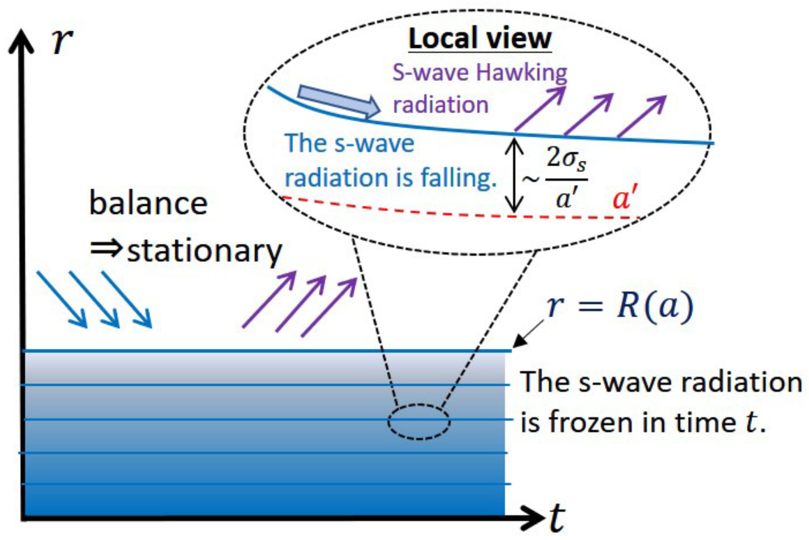
This object has the surface at , instead of a horizon. We can also check that there is no trapped region inside. However, the redshift is exponentially large inside, and time is almost frozen in the region deeper than the surface by . Therefore, this object looks like the conventional black hole from the outside. Note also that, because of this large redshift, only the Hawking radiation from the outermost region comes out although the radiation is emitted from each region inside [9].
Next, let’s consider a stationary black hole. Suppose that we put the evaporating object in the vacuum into the heat bath with temperature . Then, the ingoing and outgoing radiations balance each other, and the system becomes stationary. The object has the surface at for , which corresponds to a stationary black hole in the heat bath 18. Then, the outside spacetime is described approximately by the Schwarzschild metric (instead of the Vaidya metric):
Thus, by changing T to t through , we have [9]
which is the candidate metric for the stationary black hole. This metric is continuous at and connected to the flat region around
at by the relation .
3.2. Generalization of the Metric
The interior part of the candidate metric (61) doesn’t contain the effect of scattering which has been mentioned above (30). Actually, the metric has for , which is, through Equation (1), equivalent to . Here, and are the energy density and radial pressure, respectively. This indicates that, from a microscopic point of view, the collapsing matter and radiation move radially in a lightlike way without scattering. In this subsection, we introduce a phenomenological function representing the effect of the scattering and generalize the metric (61) [14].
3.2.1. Another Phenomenological Function
We first examine the energy-momentum flow in the general static metric (2). The self-consistent energy-momentum flow must be time-reversal, which can be characterized by
Here, is a function. As we have seen that the interior of the object is very dense, we assume that is a function of which varies slowly 19. and are the radial outgoing and ingoing null vectors, respectively:
These transform under time reversal as . Equation (63) can be rewritten as
where stands for , and so on. Furthermore, this can also be expressed in terms of the ratio between and :
Therefore, must satisfy
Here, the first inequality is required by the fact that, in Equation (65), plays a role of the ratio between two energy flows, which must be positive. The second one is needed in order for the pressure to be positive under .
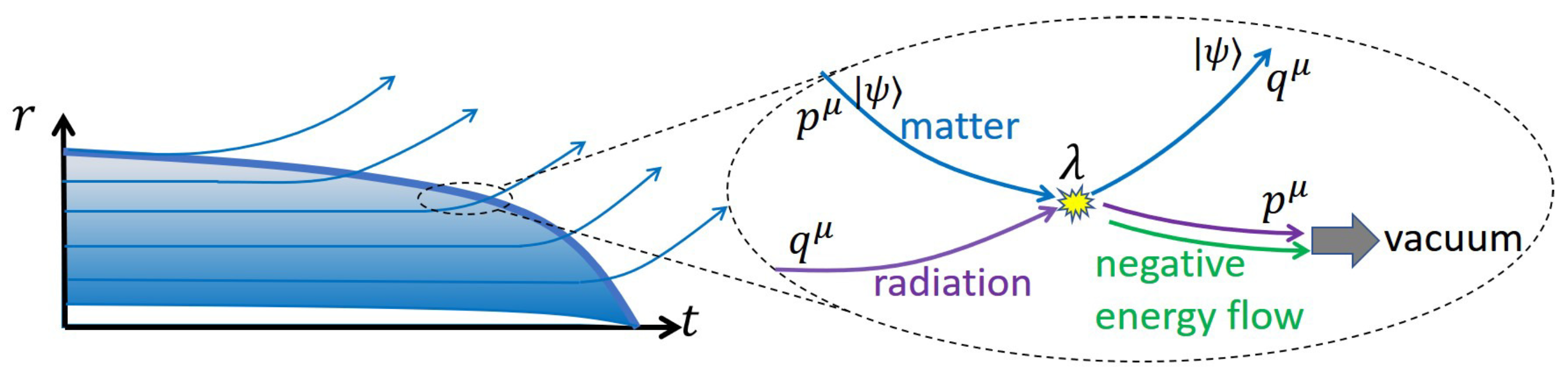
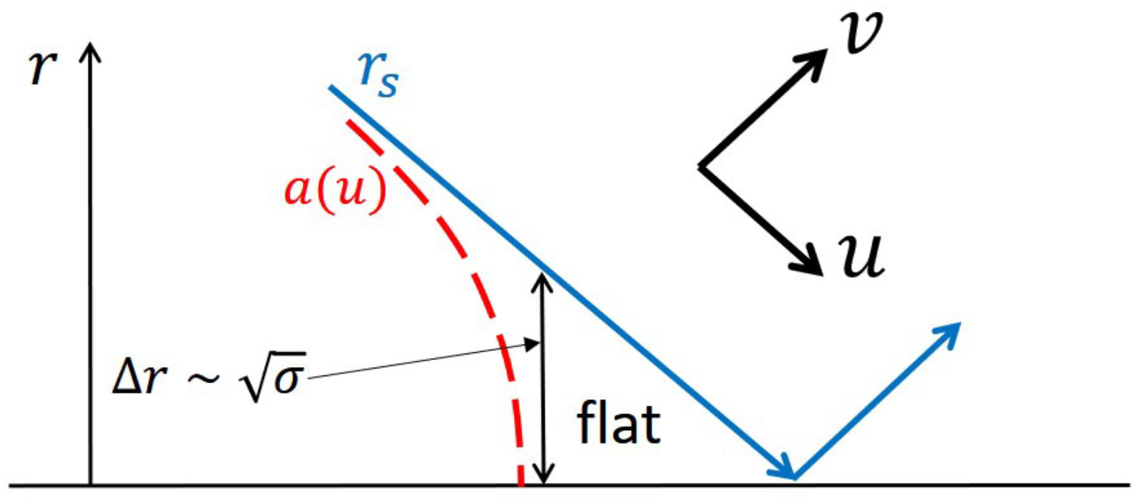
Now, we discuss the physical meaning of from a microscopic point of view. See Figure 10.
We focus on one of the null shells that make up the black hole and consider the moment when the size is r, which is represented by S in Figure 10. The vector expresses the energy-momentum flow through the shell, which moves lightlike inward along . If the radiated particle is massless and propagates outward along the radial direction without scattering, should be parallel to , which means . Therefore, represents the deviation from this ideal situation. can become non-zero if the massless particle is scattered in the ingoing direction by the gravitational potential or interaction with other matters20. This is because such a scattered particle comes back to the surface in the time scale of according to Equation (6), and produces an energy-momentum flow along the direction. In this way, is a phenomenological function that depends on the detail of microscopic dynamics.
3.2.2. The Candidate Metric
We determine and by considering the ratio (66) for a given . Here, we assume for simplicity that is a constant satisfying the condition (67) in . We can expect that the introduction of should not change the functional forms of and in a drastically different way from those of the metric (60) 21. Therefore, we can put
where and are some coefficients such that in 22.
Then, using the ratio (66) and the Einstein Equation (1), we have for
that is, . Therefore, Equation (68) becomes
At this stage, the intensity is arbitrary, and we can redefine it and remove without losing generality to obtain
This metric is again continuous at the surface at . The center is assumed again to be flat, which requires that there. The flat metric (62) around is expressed in terms of t approximately as
The metrics (72) and (73) are our candidate metric23. It depends on two parameters , which will be determined self-consistently later.
The interior part of the metric (72) can also be applied to the evaporating black hole because the interior is static. Therefore, the previous metric (57) is generalized to
We check the form of the Einstein tensor. The interior part of the metric (72) has
to for . This means through the Einstein Equation (1) that the energy density and pressure are positive, but the angular pressure is so large (almost Planckian) that the dominant energy condition violates, as mentioned in Section 1.
Next, we calculate the curvatures in :
This means that, if the metric is the solution of the Einstein Equation (1) and Equations (11) and (67) are satisfied, the geometry has no singularity. Then, the Penrose diagram of the evaporating black hole is given by Figure 1.
We here discuss Hawking radiation in this picture. We consider the total energy flux through an ingoing null shell along in Figure 10:
where Equation (64) has been used, and is the vector of the local time (like in Figure 8). This is a generalized definition of the total flux. Applying the definition (79) to the interior of the metric (72) (or (74)) and using Equations (1) and (75), we have . For the exterior part of the metric (74) for the evaporating black hole, on the other hand, we obtain . Then, we have by using Equations (1) and (5). Thus, these agree with each other at , which means that the radiation emitted from the inside goes to the outside.
Finally, we argue that the interior part of the metric (72) is locally. First, we can check that, in general, a spherically symmetric metric is spacetime with if the condition
is satisfied24. For the interior metric, we have and , where we have neglected the contribution from of for . Then, the condition (80) is satisfied for around the point r we are focusing. Thus, the interior metric can be approximated locally as geometry:
where 25. This means that the local symmetry for a fluid before the matter collapses becomes that for after the black hole is formed. It would be interesting to study this more in future.
4. Field Configurations
We consider N massless free scalar fields
in the candidate metrics (72) and (73) and study their configurations to find a candidate state. This action leads to the equation of motion26
4.1. Classical Effective Potential and Bound Modes
Before going to quantum fields, we study the classical behavior of matter to see intuitively what happens in the spacetime (72). To do that, we analyze the field Equation (83) in the classical approximation to draw the effective potential for the partial waves of the fields.
We first consider the general static metric (2) and set
where and the normalization factor will be fixed in Section 4.2. Then, the field Equation (83) becomes
This Equation (85) takes the same form as the Schrödinger equation with energy and the potential . Therefore, the classically allowed region is determined by the condition .
In general, when one studies a field equation in a curved spacetime, he needs to take the curvature effect into account, which is expressed here as the “mass term" , the two derivative term of the metric27. For the metrics (72) and (73), takes28
However, should not significantly affect the purely classical motion of matter because a classical particle equation (Hamilton–Jacobi equation) does not include derivative terms of the metric. Therefore, in this subsection, we ignore for a while.
Let us draw the classical effective potential for the whole spacetime of the static black hole with const. for simplicity. (This corresponds to the stationary black hole in the heat bath). We apply the metrics (72) and (73) to the formula (86) (without ) and obtain
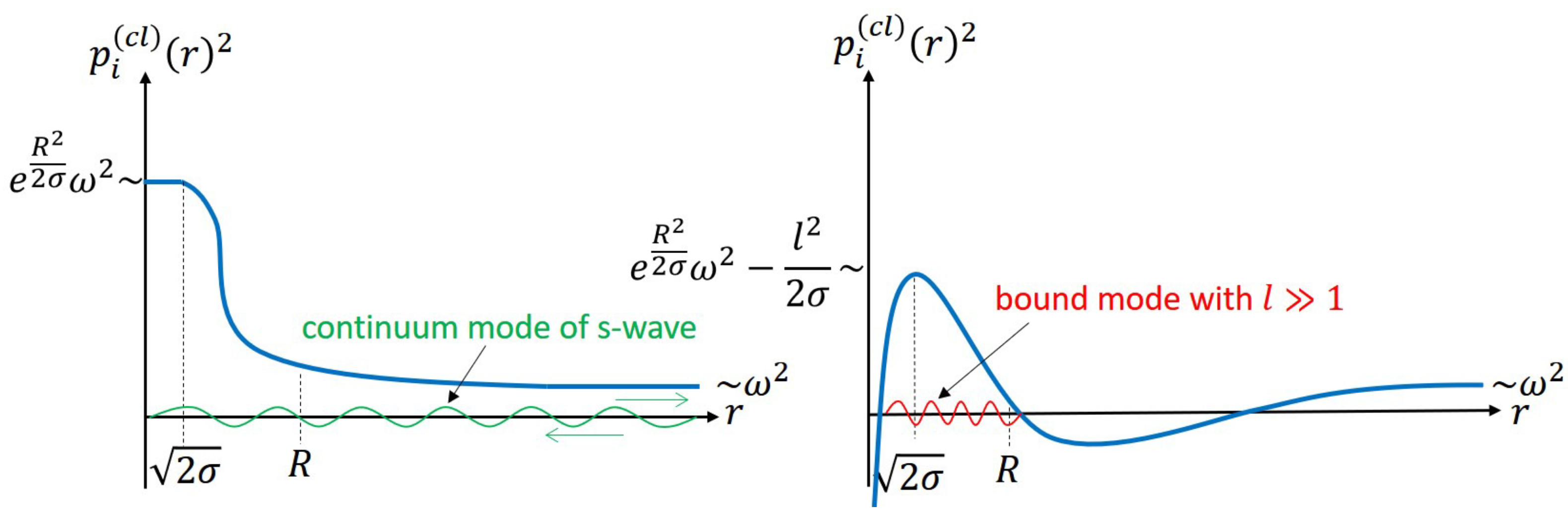
This is continuous29. Note that the frequency is measured at .
For , we have the left of Figure 11, which shows that the whole region is allowed classically; s-waves can enter the inside from the outside, pass the center, and come back to the outside, which takes an exponentially long time because of the large redshift.
We refer to such modes as continuum modes in the following. For , on the other hand, the classically allowed region consists of two disconnected domains as in the right of Figure 11. The outer one indicates that such modes coming from the outside are reflected by the barrier while the inner one shows that they are trapped inside, which we call bound modes.
Now, we discuss the behavior of each mode in the formation process of the black hole. We first study the condition for a mode with to enter the black hole with a from the outside. From the potential (88), for , we have , which becomes zero at . This means that the mode is reflected at the point and returns to the outside. Therefore, the condition is that is, . From this, we can also see that a mode with composing i-th shell of the multi-shell model in Figure 8 can enter inside if . As we will see in Section 6, most such modes have the energy . Then, the condition becomes . Thus, we conclude that only the continuum modes of s-wave can enter the black hole from the outside.
Although modes with cannot enter from the outside, they emerge inside the black hole in the formation process. To see it, we study how the potential changes for a given as a increases from zero. See Figure 12.
Initially, there is no mass, , so the spacetime is flat and the potential is given by the purple line. When the mass becomes larger than , the allowed region appears inside, which is described by the blue line. Then, the bound modes emerge there. As the mass increases, the potential grows up and the allowed region is broaden (see the green and yellow lines). Then, the outer zero point (which is depicted by the arrows) moves inward, which means that, as the mass increases, the gravitational attraction increases, allowing the mode to overcome the centrifugal repulsion and penetrate more inside. In this way, many bound modes emerge inside the black hole independently of the initial state.
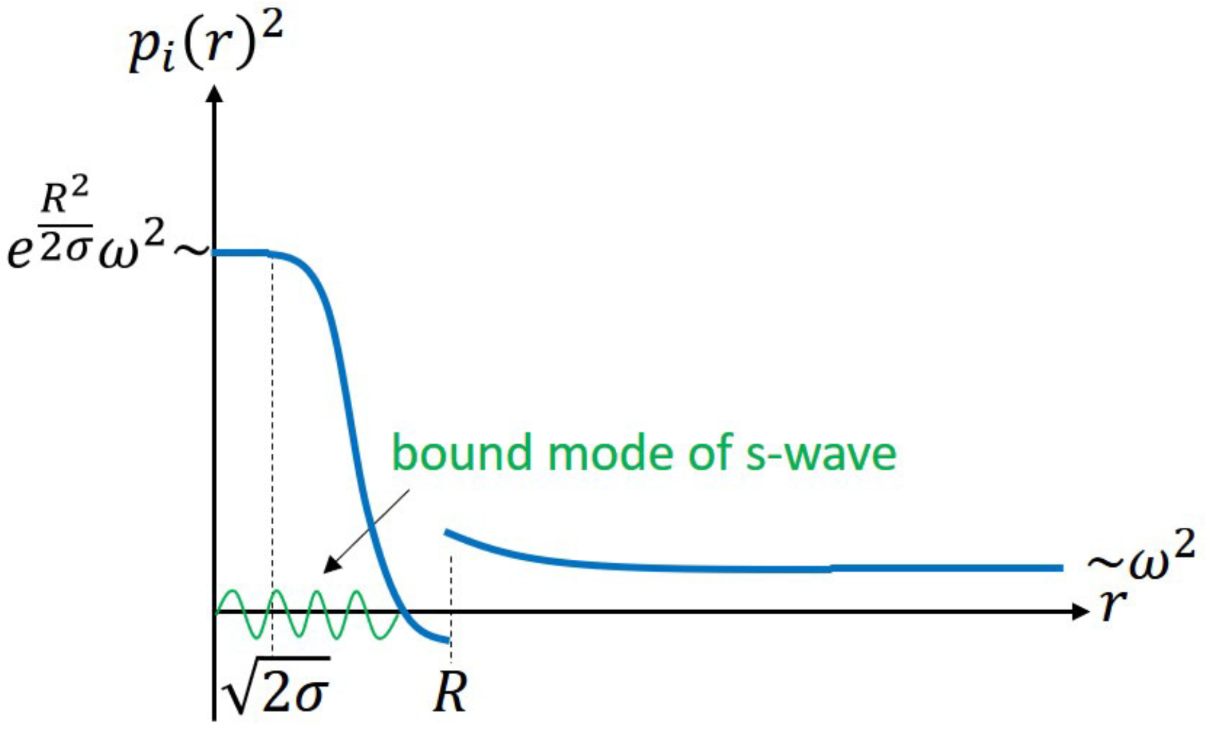
Finally, we note that, if the curvature term is considered in the formula (86), the bound mode of s-wave can also emerge inside the black hole. In fact, for , we have . This means that the s-waves with are trapped inside . See Figure 13. Thus, the s-wave in the interior metric can be in a continuum mode as in the left of Figure 11 or in a bound mode as in Figure 13.
4.2. WKB Approximation
We now consider quantum fields and try to solve the field Equation (83) by WKB method30. In the interior of the metric (72), the leading WKB solution is given, through Equations (84), (85) and (86), by [59]31
Here, , , , and is a phase factor, where labels the frequencies for each l and m. For the bound modes, the frequencies are quantized, (), and are approximately given by32
where vanishes at . The normalization is fixed as (see Appendix D)
On the other hand, the s-waves have continuum modes (as in the left of Figure 11), which we will discuss more in Section 6.
We also have the commutation relation
and
where is the momentum conjugate to :
The ground state for all modes in the interior metric is characterized by
4.3. A Candidate State
We show that the bound modes are in the ground state while the continuum modes of s-wave are in an excited state. If is the ground state for the bound modes , it satisfies
where B stands for the set of the bound modes. From Figure 12, the condition (97) is independent of the initial state of the system because the bound modes emerge in the region disconnected from the outside.
In general, the ADM energy M inside radius r in a spherically-symmetric spacetime is given by [40]
where
Then, we can define the ADM-energy increase of the first-excited state of the i-th bound mode (of a component of fields ), , by
where satisfies the condition (97) and the integration interval is the allowed region of the bound mode . This is finite because the UV divergence is subtracted by the second term. We estimate the order of this by using the WKB approximation.
We first check the condition for the bound mode to exist, which is determined by the quantization condition (91). That is, the quantum number of the i-th bound mode must be at least greater than 1:
where we have considered only the most dominant term of Equation (86) in the WKB approximation and evaluated the integration as with a constant 33. Therefore, the frequency must satisfy
Similarly, we can calculate from Equation (A20)
Next, we see from Equations (89) and (90). Using Equations (94) and (97), we can see easily . We check the form
Then, we evaluate
Here, on the first line, we have applied only to in ; on the second line, we have used the WKB solution (90), and ; and, on the last line, we have picked up only the most dominant terms because we are interested in the order estimation.
Thus, we estimate the energy increase (100) as
Here, on the first line, we have used the evaluation (105); on the second line, we have expressed with ; on the third line, we have employed Equation (103); and on the last line, we have applied the condition (102). That is, we have34
Here, as we will see in Section 6, the statistical fluctuation of the mass of the black hole is . Thus, the result (107) means that when the number of excited bound modes exceeds , the excitation energy becomes larger than , and the object becomes different from the black hole. Therefore, we can regard that the bound modes are in the ground state because is negligible compared to the number of total modes, which is on the order of (see Section 6).
On the other hand, the continuum modes of s-wave are not restricted by the condition (102) because they are not trapped inside. Therefore, those modes can enter and exit the black hole as an excitation that represents the collapsing matter and Hawking radiation. Thus, the candidate state is a state in which the bound modes are in the ground state and the s-waves are excited, leading to the energy-momentum tensor (3). (In Section 6, we will characterize more specifically).
5. Energy-Momentum Tensor in the Ground State
In this section, we evaluate of Equation (3), where is the ground state (96). The plan is as follows. In Section 5.1, we first study how the WKB approximation breaks down and solve the field equation in a different perturbation technique to obtain the leading solution of the bound modes. In Section 5.2, we check the general procedure of the renormalization for the dimensional regularization. In Section 5.3, we evaluate the leading value of the renormalized energy-momentum tensor . In Section 5.4, we study the subleading value .
5.1. Solutions of the Bound Modes
We construct the solutions of the bound modes in the interior, which will be used in Section 5.3.
5.1.1. Breakdown of the WKB Approximation
We first examine the validity of the WKB approximation in Section 4.2. If we want to evaluate the energy-momentum tensor at a point inside the object, we need at with various values of . Then, the proper frequency and the proper angular momentum at are physically important:35
In terms of these, the formula (86) is expressed as
From this, we have . This means that the WKB approximation is good at for because the semi-classical treatment is valid for a large wave number: [59]. On the other hand, the approximation is bad for ; becomes the turning point. Although the WKB approach has a potential to reproduce the UV-divergent structure of the energy-momentum tensor properly, it cannot determine the finite values without errors36.
For later analysis, we investigate more precisely how the approximation breaks down. In oder for the WKB analysis to be valid, the wave length must change slowly [59]. We pick up only the first term of Equation (109) because the exponential factor changes most drastically as a function of r. We then evaluate at
where the derivative has applied only to the exponential. If , the approximation at is good for and bad for , which is consistent with the fact that the curvature radius is from the Ricci scalar (76). The evaluation (110) tells more: even when , the approximation is good at if is inside the turning point so that is satisfied, that is,37
5.1.2. A Perturbative Method and the Leading Exact Solution
The finite values of the energy-momentum tensor are important for our self-consistent discussion. We here develop a new perturbation method to solve exactly the field Equation (85) in the interior of the metric (72). Suppose that we want to determine at a point . Motivated by the evaluation (111), we set
and expand the potential (109) as
where and are considered as , and s is an expansion parameter. is the leading potential of , and is the subleading one of . Note here that cannot be expanded because its exponent is .
Now, we can determine around by the perturbative expansion with respect to . We put it as
Combing this and Equation (113), then the field Equation (85) becomes
This gives an iterative equation:
By construction, is the leading exact solution in this perturbative expansion.
Let us solve the leading Equation (116). We can convert from x to
and rewrite the Equation (116) as
where
This is the Bessel equation, whose solutions are Bessel functions and . Using the boundary condition that the mode is bounded, we can choose properly. Considering the evaluation (111) and the region where the WKB solution (90) is valid, we can fix the normalization. See Appendix E. Thus, we obtain the leading solution
Substituting this and the normalization (92) for the formula (84), the leading bound-mode functions in the interior of the metric (72) without (which will not affect the following analysis) are given by
Note again that depends on and A on l.
The subleading solution can be determined from the subleading Equation (117) and the leading solution (121), for example, by the Green-function method. We leave it as a future task.
Finally, we make a comment on the origin of the leading potential . We can also focus a region around and use the metric (81) to show that the field Equation (83) becomes the Bessel equation. In this sense, the local structure makes the Equation (83) solvable. More generally, the condition (80) is the origin.
5.2. Dimensional Regularization and Renormalization
In general, when one considers composite operators such as , he needs to regularize them. We use the dimensional regularization technique, which has an advantage that it is covariant; thus, it is the UV-divergent part. Before going to the explicit evaluation of , we here give the general discussion about the dimensional regularization and renormalization of the energy-momentum tensor.
The bare action of our theory on a d-dimensional spacetime is
where the index B expresses the bare quantities.
First, we don’t consider quantization of gravity, and the quantum scalar fields are free. Therefore, the bare fields are the same as the renormalized ones:
Next, we introduce a renormalization point . Because there is no mass in the theory, the renormalization of the Newton constant does not appear. Therefore, by dimensional analysis, we can put
where , and G is the 4D physical Newton constant, which is independent of . agrees with G in . On the other hand, , , and need to be renormalized. In the limit , they take the form
Here, we choose the counter terms with as those which are required to renormalize the UV-divergent part of the effective action of N massless free scalar fields by the minimal subtraction scheme [41,42,60]. , , and are the renormalized coupling constants at a renormalization point .
Then, the equation of motion for , =0, is given by
Here, is the regularized energy-momentum tensor operator, which is formally given by Equation (99) with replaced by the d-dimensional matter action of the bare action (123). The other tensors are proportional to the identity operator, which are given by
From this, we can obtain the precise expression of the Einstein Equation (1):
Here, we have defined
where the 4D renormalized energy-momentum tensor at energy scale is
This is finite in the limit , as we will see explicitly below.
The second term in the r.h.s. of the definition (132) is a finite renormalization which plays a role in choosing the theory. The point is that the -dependence of the renormalized coupling constants must be chosen so that the bare coupling constants are independent of . From the formulae (126), the condition provides in . We can do the same procedure for the other couplings. From these, we obtain
5.3. Leading Terms of the Energy-Momentum Tensor
Now, we evaluate the leading value of the renormalized energy-momentum tensor (132) for , . Generically, the continuum modes of s-wave also appear in the mode expansion of a field . However, as we will see in Section 5.3.2, the leading value becomes by integrating both and l, which means that the sum of such s-wave modes (integration only over ) can contribute to at most . Therefore, in this subsection, we keep only the bound modes (122) in the expansion of the leading solution of .
5.3.1. Fields in the Dimensional Regularization
To use dimensional regularization, we consider the -dimensional spacetime manifold , where M is our 4D physical spacetime and is -dimensional flat spacetime [61]. That is, we take
In this metric, the leading bound mode function (122) becomes
The plane wave part makes a shift in the formula (86), and the definition of the label A changes from Equation (120) to
5.3.2. Renormalized Energy-Momentum Tensor
From the leading solution (138), we can obtain the leading values of the regularized energy-momentum tensor (see Appendix F for the detailed calculation)38:
where the components are in the order of and
Here, is Euler’s constant and c is the non-trivial finite value for :
Note here that, as shown in Appendix F, this leading value of is obtained as a result of the integration over and l, and the 4D dynamics is important.
Next, we can check that the poles of Equation (139) are cancelled by the counter terms in Equation (133), and is indeed finite. Here, we have used the explicit form of , and for the interior part of the metric (72):
Finally, we use the definition (132) with the running coupling constants (134) to obtain the renormalized energy-momentum tensor with a finite renormalization:
where
Here, the -dependence disappears. In Section 7, we will see that and should be tuned properly in order to have a self-consistent solution of the form of Equation (72).
The point is that the leading value of the trace is fixed independently of :
We can see that this comes from the UV-divergent structure and is essentially the 4D Weyl anomaly [41,42,62] although the matter fields are not conformal. The value (145) was obtained by first renormalizing the divergences and then taking the trace. We can reverse the order to see clearly how the value appears. If we first take the trace of , we have, through Equations (99), (A72), (A78), and (A83),
before taking the limit . However, the trace of the counter terms in the definition (133) makes a non-trivial contribution:
where we have used Equations (76), (77), (78) and
5.4. Sub-Leading Terms of the Energy-Momentum Tensor
The sub-leading bound-mode solution of Equation (117), which we have not found yet, determines the subleading value completely40. In this subsection, we instead use the conservation law to show that is expressed in terms of two parameters.
In the interior part of the metric (72), the conservation law is expressed as
where is assumed to be static and spherically symmetric: and 41.
, , and are conserved, and their explicit forms are given by Equation (142), which are negative power polynomials in starting from a constant. In addition, the leading value is constant. Motivated by these facts, we can set the ansatz as
By construction, should be a -independent finite number of , as we have seen in the leading value (144). We suppose that such a is given. By using Equations (143), (144), the second one of (153), and (155), we can obtain
Finally, we write the subleading value of the trace part as
where is a finite value independent of the finite renormalization in the definition (132) because of Equation (142). We suppose that such a is obtained. This together with Equations (154) and (156) determines .
Thus, we can express all the components of to in terms of .
6. Contribution of S-Wave Excitations to the Energy-Momentum Tensor
In this section, we first consider the generic configuration of excitations of the continuum modes of s-wave from a statistical point of view and characterize the candidate state more. Then, we study the excitation energy in the interior of the black hole and find the energy density . From this and the conservation law, we infer of Equation (3).
6.1. Fluctuation of Mass of the Black Hole
We consider the black holes with mass that are most likely to be formed statistically. Such black holes are created in the most generic manner. When making a black hole in several operations, the more energy given per operation, the more specific and less generic the black hole formed is. Therefore, the most generic black hole should be created by using a collection of quanta with as small energy as possible. According to Bekenstein’s idea [46], in order for a wave to enter the black hole, the wavelength must be smaller than a: . This means that the energy of the wave, , must satisfy . As discussed in Section 4.1, only continuum modes of s-wave can play a role in the black-hole formation. Therefore, a quantum required is such a s-wave with the minimum energy,
Suppose that we form a black hole of size a by injecting such quanta many times. Because the wavelength of each quantum is almost the same as the size of the black hole at each stage (), the wave enters the black hole with a probability of 1/2 and is bounced back with a probability of 1/2. Here, we model the formation as a stochastic process according to binomial distribution. Then, the average number of trials is given by dividing by the energy that can enter at one time:
This means that all the black holes with mass are not statistically distinguished, and they are considered as the same macroscopically.
6.2. S-Wave Excitation inside the Black Hole and
To determine the functional form of , we consider how the s-wave excitations used to form the black hole are distributed in the interior part of the metric (72). First, suppose that an s-wave having a proper wavelength is excited at a certain point r inside the black hole. It has the proper energy . Here, the local Hamiltonian is given by , where is the proper length of a width around r, is the energy-momentum tensor from the contribution of the excitation, and is the proper time of the local inertial frame at r. Therefore, by considering the number of fields N, we can set and and obtain
Here, holds because we have in the local inertial frame. Furthermore, in the static metric (72), we have . Thus, we reach
Using this and the formula (98), the ADM-mass contribution from this excitation can be expressed as
Here, on the first line, we have divided it by N because the s-wave is an excitation of one kind of field and contains all the contribution from N kinds of fields; and on the last line, we have used for the interior of the metric (72). According to the formation process in the previous subsection, each s-wave excitation corresponds to the ADM energy (158)42. Therefore, the condition indicates
and then the energy density (162) becomes
where we have used . This should be the self-consistent form. In Section 9, we will discuss how to obtain this functional form from the field equation.
We here discuss the entropy from this point of view. We consider a unit with width inside the black hole. It contains N waves with because the proper wavelength (164) corresponds to and the ADM mass of the unit is evaluated from the energy density (165) as . Therefore, the entropy per proper radial length, s, can be evaluated as
which means that bits of information are contained per proper length. On the other hand, the proper length of the interior of the black hole is evaluated from the metric (72) as
which is much longer than a. Thus, the entropy is evaluated as
6.3. The Form of
Using the form of (165) and the conservation law inside the black hole (151), we express all the components of in terms of a single parameter . First, by the same reason as , we can set the ansatz for as Equation (152):
Now, Equation (165) shows that is at most order of , which means . The first one of Equation (170) indicates . Next, as seen in Section 5.3.2, the leading order appears as a result of the integration over . Therefore, , which represents the contribution of the s-wave excitation, should be smaller than . This requires , and then the second one of Equation (170) leads to . Thus, all the components are at most order of , which can be expressed as
Here, are the ratios between terms of and which are determined by dynamics of the s-waves including the contribution from the negative energy flow (see Section 9).
Then, the third one of Equation (170) determines as
Thus, all the components of are expressed in terms of the parameter under a given . Note that corresponds to the square of the amplitude of the classical field that represents the collapsing matter and radiation. For a later convenience, we represent in terms of a parameter as
7. Self-Consistent Solution
We have obtained all the ingredients for the self-consistent analysis: the candidate metric (72), which is written in terms of , the energy-momentum tensor for the ground state (143), (154) and (157), which depend on , and the energy-momentum tensor for the s-wave excitation contribution (171), which is controlled by . In this section, we solve the Einstein Equation (131) and determine the self-consistent values of for a certain class of . We then examine the consistency.
7.1. Self-Consistent Values of for a Class of
First, we examine the trace part of the Einstein Equation (131), , to . It is obtained from Equations (76), (145), (157), and (171) (with Equations (172) and (173)) as
Equating the terms of on the both sides, we have , that is,
This is indeed proportional to , which is consistent with the assumption we have put just below Equation (5). In addition, appears in the denominator, and with is smaller than that with , which is consistent with the meaning of in Figure 10. Then, the terms of in Equation (174) together with the result (175) bring , which means
First, the terms of are balanced on the both sides if and are tuned such that
Then, the terms of lead together with the intensity (175) to
Note that the -component and -component of the Einstein equation hold automatically because of the conservation law and the trace equation.
Here, should be chosen so that the condition (67) is satisfied. Note that is actually constant, as we have assumed in Section 3.2.2.
Thus, we have determined the self-consistent values of in terms of that can be fixed in principle by dynamics (see Equations (154), (157) and (171) for their definitions). Therefore, the interior of the metric (72) and the state are the self-consistent solution of the Einstein Equation (1). Note that this is a non-perturbative solution w.r.t. ℏ because we cannot take in the solution metric (72) with the values (175) and (180).
7.2. Consistency Check
First, we check the curvature . From Equations (76), (77), (78), and (175), we can evaluate
which is smaller than the Planck scale if N is large, Equation (11)43. Thus, no singularity exists inside the black hole44 and the Penrose diagram is actually given by Figure 1. Note that this result is so robust because (175) is not affected by the values of .
Second, we study the energy density. From Equations (144), (154), (171) (with (173)), (180) and (181), we have
to which both and contribute. Integrating this over the volume in the formula (98), we can reproduce the total energy M. We also see from the definition of the energy flux (79) that the energy density (183) also leads to the Hawking radiation consistently. Therefore, both the bound modes and s-waves play a role in the energy inside the black hole.
Third, we discuss the tangential pressure. The self-consistent solution has
which can be checked by Equations (143), (171), (175), and (178). From this, we can see that this near-Planckian pressure comes from the vacuum fluctuation of the bound modes in the ground state. The origin is the same as the 4D Weyl anomaly because the value (184) comes from the second term of Equation (143), which appears from the pole as shown in Equation (A86). Indeed, twice that of the pressure (184) is equal to the trace (145). Therefore, the pressure is very robust in that it is independent of the state. Note also that this large pressure supports the object against the strong gravity, which can be seen by noting that in the conservation law (151) and are balanced for the self-consistent solution.
This large tangential pressure associated with the anomaly should be universal for any kind of matter fields. In the previous work [24], only conformal matter fields were considered, and the 4D Weyl anomaly was used to obtain the self-consistent solution with the large tangential pressure. In the present work, however, we reach the same picture of the black hole without using the conformal property, which means that the assumption of conformal matter is not essential. It is related to the fact that any matter behaves as ultra-relativistic near the black hole, as we have discussed around Equation (6). Therefore, our picture of the black hole should work for any kinds of matter fields. Even for a massive field, it should if the mass is smaller than .
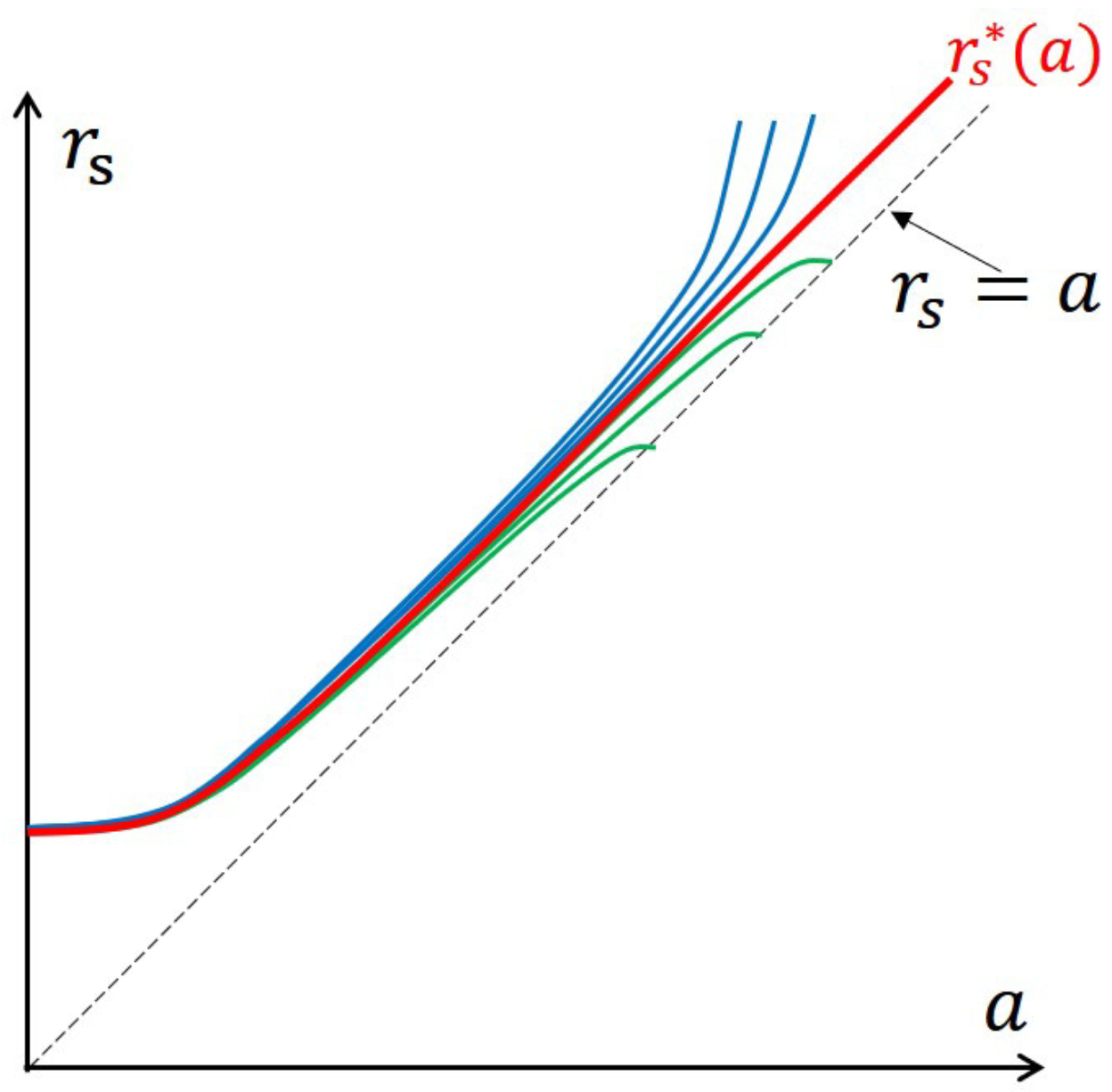
The surface pressure (49) also comes from this tangential pressure. When a shell in Figure 8 approaches so that Equation (8) is satisfied, the interior metric becomes Equation (72) and the shell itself forms a new surface, whose position is represented by the point R in Figure 11. Then, the vacuum fluctuation of the bound modes which reach the point R produces the tangential pressure (184), which corresponds to the continuum version of . Note that the mode that makes the pressure is different from the mode that constitutes the shell while the surface pressure (49) has been obtained by a geometrical analysis. Therefore, the two modes are combined to form the consistent picture.
Finally, we discuss the finite renormalization. In this solution, there are no quantities with dimension other than . The value (175) implies that the renormalization point should be chosen near the Planck scale:
Then, the condition (178) means that . On the other hand, the solution (180) together with the condition (67) indicate that . Therefore, we have
From this and the curvature (182), we can see that all four of the terms of gravity in the bare action (123) are . Therefore, the terms cannot be much larger than the R term, which means that the three terms would not change the picture of the black hole drastically even if we consider them from the beginning45. Thus, our argument based on the Einstein–Hilbert term is self-consistent.
As we have seen, the coupling constants and should be related by Equation (178). However, there is a possible way to relax it. Instead of the interior metric (72), we consider and , where is a small number. Because this ansatz satisfies the condition (80), we can solve the wave Equation (83) locally as discussed in the end of Section 5.1.2. Then, we can evaluate the renormalized energy-momentum tensor , which should contain -dependent terms. Therefore, we should be able to choose so that the terms satisfy the Einstein Equation (131) for a given value of . It would be exciting to find another class of solutions in this direction.
8. Black Hole Entropy
We count the number of states of the s-waves inside the black hole to evaluate the entropy more quantitatively than the discussion in Section 6.2.
8.1. Adiabatic Formation in the Heat Bath
Let us consider the adiabatic formation of the black hole in the heat bath [14]. Specifically, suppose that we grow a small black hole to a large one very slowly by changing the temperature and size of the heat bath properly46. Then, we obtain the stationary black hole, whose metric is given by Equation (72) with const., and consider it as consisting of excitations of the s-wave continuum modes, as discussed in Section 6.
This black hole is not in equilibrium in an exact sense [16]. Let us see the above formation process from a microscopic view. See Figure 14.
At a stage where the black hole has the radius , s-wave ingoing radiation from the bath comes to the black hole, balancing s-wave Hawking radiation of with the s-wave intensity (13). The ingoing radiation approaches
as we have shown (8). Then, the local temperature that the radiation feels there is
which is near the Planck temperature because of Equation (13). After this, the subsequent radiations pile up and cover the radiation. Then, it is redshifted exponentially, almost frozen in time t, and suspends there. From the local point of view, however, the radiation keeps falling with the initial information. Therefore, the black hole is not in equilibrium in the usual sense. Rather, the ingoing radiation from the bath and the Hawking radiation are just balanced, and therefore the system is stationary.
This property allows us to use the temperature (188) as the local temperature at each radius r inside the black hole. Because of the exponentially large redshift, the outgoing Hawking radiation there is frozen in time t. Even if we wait for an exceptionally long time which is longer than the lifetime of the universe, the Hawking radiation of this temperature (188) will not go outside to exchange energy with the radiation from the heat bath. This indicates that Tolman’s law [63] doesn’t hold inside the black hole47. As we will see below, this is consistent with the area law of the entropy.
8.2. Micro-Counting of the S-Wave States
We count the number of possibilities of these s-wave configurations to find the entropy density per radius r inside the black hole. First, we evaluate the number of the s-waves with frequency in the width near the surface when the black hole of is formed. In the semi-classical approximation [59], using the condition (91) for , , , and , we can evaluate for N kinds of fields 48
Here, is the blueshifted frequency when approaching the surface, and we have approximated near the position (187). Thus, the number of modes for is given by
Next, we review the entropy of a harmonic oscillator with frequency in the heat bath of temperature [63]. The canonical distribution is given by , where
Therefore, the entropy is evaluated as
where we have defined a function
From the formulae (190) and (192), we obtain the entropy density:
with (188). The reason of the factor is that, because of the time-freezing effect, only ingoing modes carry the information, and the integration only over ingoing direction momenta should be performed. This can be evaluated as
where on the third line we have used the intensity (13)49. Integrating this over the interior reproduces the area law:
where and have been used50. This implies that the information is stored inside the black hole as excitations of the s-waves.
9. Mechanism of Energy Decrease of the Collapsing Matter
In this section, we examine how the energy of the collapsing matter decreases and discuss how , Equation (171), is obtained by dynamics. The point is to consider the contribution from the vacuum fluctuation of s-waves.
9.1. Setup
Suppose that a classical matter collapses to the black hole which is described by the self-consistent metric. To analyze the time evolution of this matter, we can focus just on the part of the matter around the surface, since the deeper region is frozen in time due to the exponentially large redshift. We consider the matter as consisting of many shells like the multi-shell model of Figure 8 and study the energy of the outermost shell along as in Figure 15.
We use the Vaidya metric (4) in the coordinate to describe the outside region:
where follows Equation (5) and each function is given by
We label the outermost shell by so that its location is given by .
9.2. S-Wave Model of Quantum Fields
Thus far, we have considered the collapsing matter as an excitation of s-waves, and we have also seen that only s-waves can enter and exit the black hole. Therefore, in order to study quantum fields propagating in this time-dependent background spacetime, we can use the s-wave approximation to analyze N massless free scalar fields as we have done in Section 251. In this subsection, we explain the general setup [41,56].
We consider s-waves of N kinds of scalar fields, , in a spherically symmetric metric, where is the 2D part of the coordinate. The 4D action can be reduced to the 2D one:
where r is the areal radius, and the derivative is applied only to as the approximation. Here, we have defined the 2D field as
The 2D energy momentum tensor is given by
which is related to the 4D energy-momentum tensor through the definition (200) as
Classically, this 2D part is traceless, . However, the 2D Weyl anomaly contributes to the trace part [41,56]:
where is the 2D Ricci scalar.
We here consider a 2D metric of the form . Then, the 2D action (199) becomes , and the equation of motion is
Each component of the energy-momentum tensor is given from Equations (201) and (203) by
where we have used . The conservation law is given by
In the following, we consider as the expectation value with respect to a state . The information of is introduced as a boundary condition of .
9.3. Hawking Radiation
Now, let us find in our setup of Figure 15. Initially, , and there is only the collapsing matter with . Therefore, appears as a result of dynamics of the quantum fields.
First, we can use the third one of Equation (205) to express the conservation law (206) as From this, we obtain
Next, we determine by the boundary condition given above Equation (33). That is, the quantum fields have started in the Minkowski vacuum state from a distance (see the left of Figure 15)52. This corresponds to the condition that , where U is the outgoing null time in the flat region around . In general, in order for to transform covariantly under , this holomorphic term must change as [55,56]
Thus, Equation (208) becomes
The shell we are now considering corresponds to the outermost one in the multi-shell model of Section 2.3.2. Therefore, we can use the result (53), that is,
Calculating the first two terms of the formula (210) from Equation (198) and evaluating with the relation (211) in the same way as in deriving Equation (45) from Equation (42), then the formula (210) becomes
where the last two terms come from . This formula can be applied to any point outside the black hole.
On the other hand, vanishes near the surface at :
which is consistent with the literature [41,50,51,53].
Thus, the Hawking radiation of the s-waves is created at () and emits the energy of the system. As we will see in the next subsection, a negative ingoing energy flow with the same magnitude as the outgoing one (213) is induced near , and the energy inside decreases as . This fact justifies the use of the Vaidya metric in studying the motion of a particle near .
9.4. Ingoing Negative Energy Flow Near the Surface
In turn, we determine the ingoing energy flow by using the conservation law (207). From Equation (198), we have , which gives through the third of Equation (205). From this and Equation (198), we can express the conservation law (207) as . Therefore, we obtain the general expression
Let us focus at . Then, the boundary term represents the energy of the outermost shell that comes from a distance at . The shell is classical, and the configuration is an ingoing solution of the field Equation (204) so that is non-zero only around and zero otherwise. We then put this classical ingoing energy flow as an idealization
where W is a positive constant. This indicates that the energy of the matter is kept along a line of .
Now, suppose that this shell comes close to at a time . Then, we can evaluate
and obtain for
where (see Appendix G for the derivation). The first negative term has the same absolute value as the outgoing energy flux at infinity (213) [41,50]. In addition, we can check that the 4D energy density of this negative part is on the order of (see Equation (226)).
The mechanism for reducing the energy of the system is as follows (see Figure 15). First, the collapsing matter comes with the positive ingoing energy . As it approaches the black hole, the negative energy flow is created from the vacuum fluctuation of the s-waves and superposed on the matter. At the same time, the same amount of the positive energy flow is emitted to infinity. Thus, the negative energy cancels the positive energy of the matter locally, and the energy of the system decreases. We can also see how this occurs in the interior metric (see section 5 of [14] and section 4-E of [16]) 54.
9.5. Configuration of S-Wave and
Here, by considering the above mechanics of the energy decrease, we discuss how to obtain in Equation (171) directly from dynamics of fields.
We first point out that the energy of the outermost shell in the multi-shell model decreases exponentially in the time [16] (see the right of Figure 15). This is the same statement as Equation (27) (or Equation (28)) in Figure 7. Here, note that in Figure 7 and Figure 15, the roles of and are reversed! Therefore, by almost the same calculation as the evaluation (29), we have in the case of Figure 15
This is the self-consistent time evolution of the energy of the matter that has come from the outside and become a part of the evaporating black hole.
The behavior (219) can be understood as a combination of the increase of the energy of the classical matter and the decrease of the energy by the negative energy flow:
where the first and second terms are the classical and quantum contributions, respectively. We explain these terms below.
First, it is natural that, when we throw a particle to the evaporating black hole, the energy of the particle itself increases if we don’t consider any quantum effect. This is because when viewed from a distant, the approaching particle is pulled by the gravitational force of the “escaping" surface of the black hole and thus gains the extra kinetic energy just like gravity assist for spacecraft. In fact, we can consider the contribution only from the ingoing energy (216) of the classical shell and evaluate the Bondi mass as (see Appendix H)55
from which we have the classical evolution of the mass
where we have used Equation (5). This gives the first term in Equation (220).
Second, we evaluate the contribution of the negative energy flow that directly reduces the energy of the shell. As we have seen in the previous subsections, the amount of the negative energy flow near the black hole is the same as that of the positive energy flow going out. Thus, the contribution we should take is equal to the difference between the energy flows and exiting the systems with mass and , respectively (see the right of Figure 15). More precisely, it is given by
where we have considered the two redshift factors in order to translate in terms of u. This can be evaluated as
Here, on the first line, Equation (213) has been applied to both and because the relation (211) holds for both u and ; on the second line, Equation (8) has been used; and on the last line, the intensity (13) has been considered. This provides the second term of Equation (220).
Now, we discuss the energy density. As shown in Appendix H, the energy density corresponding to the mass (221) is given by
while the energy density corresponding to the negative energy flow in Equation (218) is evaluated as
where we express these in the coordinate of the metric (197)56. These are not consistent with in Equation (171).
However, the above observation (220) implies that there should be a way to include the effect of the negative energy flow in solving the field equation of the s-wave. Such an analysis could be similar to “Lorentz friction”. While the radiation is emitted directly from the particle in the case of the Lorentz friction, the negative energy flow in our case is induced through the change of the metric by the motion of the shell. In this sense, these might be qualitatively different. It should be useful to consider from a field-theoretic point of view the discussion of Section 2.2, which determines the time-evolution of both the spacetime and the energy and motion of the shell. Then, we should be able to obtain the proper functional form , and the form of (171) will be determined together with . We will consider this problem in future (see also the end of Section 11).
10. Conformal Matter Fields
As a special case, we consider conformal fields as the matter fields in the Einstein Equation (1)57. In the previous work [24], we have investigated this case and constructed the self-consistent metric. Here, we perform further analysis to completely determine .
10.1. Self-Consistent Values of for Conformal Matter Fields
The key equation is the trace part of the Einstein Equation (1). The trace of the energy-momentum tensor is given by the 4D Weyl anomaly, independently of the state [41,42,62]:
with
where is the Weyl curvature and is the Gauss–Bonnet density. The coefficients and are fixed only by the matter content of the action, as we will give explicitly below, while also depends on the finite renormalization.
We can use the interior metric (72) because the multi-shell model is independent of the matter content. Using Equations (76), (77), (78), and (150), the self-consistent Equation (227) becomes
to . Note that does not contribute here because of from Equation (150). Equating the terms of on the both sides, we reach [14,24]
which is similar to the value (175). Next, comparing the terms of and using the result (230), we can obtain easily
which is a new result 58. Note here that this result is not influenced by a finite renormalization because from Equations (148) and (150). Thus, the interior metric has been determined completely only by the matter content, independently of the state and the theory of gravity.
10.2. A New Constraint to the Matter Content
We discuss the meaning of the result (231). First, the explicit values of and are given by
where , , and are respectively the numbers of scalars, spin- Dirac fermions and vectors in the theory [62]59. Using this, the result (231) can be expressed as
For example, we can see
The consistency condition of is given by Equation (67): . The lower limit has come from the positive definiteness of the ratio of the scattered part of the radiation as in Figure 10, while the upper limit has been derived by the positive definiteness of the radial pressure in Equation (66) 60. None of the above examples meet the condition.
Let’s examine whether various theories satisfy the condition (67). The first one is the Standard Model with right-handed neutrino61. It has , , and , and then the formula (233) becomes
which satisfies the condition (67). On the other hand, if we remove right-handed neutrino, changes to , and then the formula (233) gives
which is outside the condition (67). This result suggests that the right-handed neutrino should exist.
Next, we consider supersymmetric theory. In this case, we have , , and , and the formula (233) leads to
which satisfies the condition (67). Instead, if we apply the formula (233) to supersymmetric theory with vector-multiplet, which has , we get
which does not meet the condition (67).
In this way, the condition (67) with the formula (233), which is a result of the self-consistent solution of the evaporating black hole, can provide a constraint to the matter content and classify effective field theories. The weak-gravity conjecture tells that black holes should evaporate without global symmetry charge [47,48]. Therefore, Equations (67) and (233) may play a similar role62. It would be exciting to study phenomenology using them.
11. Discussion and Conclusions
In this paper, we have solved time evolution of the collapsing matter taking the full dynamics of the 4D quantum matter fields into account in the semi-classical Einstein equation. Then, we found the self-consistent metric and state . This solution tells that the black hole is a compact dense object which has the surface (instead of horizon) and evaporates without a singularity63. It consists of three parts. One is the vacuum fluctuation of the bound modes in the ground state, which produces the large tangential pressure supporting the object. Another one is the excitation of the s-waves composing the collapsing matter, which carries the information responsible for the area law of the entropy. The other one is the excitation of the s-waves producing the pair of the outgoing Hawking radiation and the ingoing negative energy flow, which decreases the energy of the matter. These three energy-momentum flows are conserved independently if there is no interaction among them.
Now, we would like to ask: How is the information of the collapsing matter reflected in the Hawking radiation and recovered in this picture? There are two remarkable points to answer this. One point is interaction between the outgoing Hawking radiation and the ingoing collapsing matter. As described in the basic idea of Section 2 and below Equation (183), the Hawking radiation is emitted outwards from each region inside the black hole. Then, the collapsing matter may collide with the outgoing radiation coming from below, go outwards, and exit from the black hole together with the information. See Figure 16.
Because the energy scale there is near the Planck scale (from Equations (182), (185), and (188)), some string-theory effect may be relevant and any kind of matter may interact with the radiation universally 64. Actually, we can describe this idea by a classical -model and evaluate the scattering time scale as
where is the dimensionless coupling constant (see Section 3 of [16]). Then, the scattering is an elastic collision in the radial direction, and the two particles swap their momenta (the right of Figure 16). Therefore, we expect that the energy distribution of the coming-back matter follows the Planck distribution of with a small correction that depends on the initial state.
This scattering process is stochastic. If an outgoing matter in the deep region goes out while the other remains inside, the matter would collide many times before going out, so the probability is very small. Therefore, the information returns in order from the surface region during the evaporation as if one peels off an onion65 (left of Figure 16).
The other point is the role of the negative energy induced by the vacuum. If the black hole evaporates and the information comes out by the above mechanism, the state along an ingoing line should approach a vacuum state (see the right of Figure 16). When the negative energy is superposed on the matter and decreases the energy, interaction between them should play a role in this evolution of the state. This point may be related to the problem of finding the correct configuration of the s-waves discussed in Section 9.5. We will study this scenario in future.
Author Contributions
All the authors have contributed to the research reported in this work and the writing of the manuscript. All authors have read and agreed to the published version of the manuscript.
Funding
Y.Y. is partially supported by the Japan Society of Promotion of Science (JSPS), Grants-in-Aid for Scientific Research (KAKENHI) Grants No. 18K13550 and 17H01148. Y.Y. is also partially supported by the RIKEN iTHEMS Program. All authors have read and agreed to the published version of the manuscript.
Acknowledgments
We thank Pei-Ming Ho for valuable discussions.
Conflicts of Interest
The authors declare no conflict of interest.
Appendix A. Motion of a Particle near the Evaporating Black Hole
For a self-contained discussion, we review the derivation of the asymptotic behavior (8) [9,14,16,24]. Equation (7) can be solved exactly by coefficient change method. The general solution is given by
where is an integration constant. The typical time scale of this equation is from the exponent, while that of is from Equation (5). Therefore, and can be considered as constants in the time scale of , and the second term can be evaluated as
Appendix B. Behavior of rs in the Limit a→0
In this Appendix, we assume the Vaidya metric (4) with Equation (5) to study the behavior of at the moment when vanishes68. Here, follows the equation of motion (6). Combining Equations (5) and (6), we obtain
This provides the relation of and a. Note that time evolution is in the direction in which a decreases. Here, we focus on the integral curves that start from points satisfying . See Figure A1.
Figure A1.
Integral curves of Equation (A2) that start from points satisfying . As Equation (A2) shows, their slopes are positive for and become zero at . They are attracted by an asymptotic curve . We can check this easily by a numerical analysis.

The curves are attracted by an asymptotic curve , which is the curve starting from (red curve in Figure A1). By numerical calculation, we can check that
for various initial values. This means that, when a becomes zero, is not zero.
In Figure A1, the blue curves are of interest to us. We are now considering a particle of those which compose the outermost part (shell) of the collapsing matter. Therefore, the particle comes from the ouside of , which the blue curves describe. On the other hand, the green curves are not physical. They start from points on and would correspond to particles coming from the inside of although the metric (4) can be applied only to the region of .
Let us construct approximately the asymptotic curve . In the stage where , the solution (A1) means that particles near approach to, in the time scale
Here, for simplicity, the lower limit value has been taken as one giving the minimum value of : . On the other hand, when , we can approximate Equation (A2) as
where we have taken in the numerator of Equation (A2) for . Then, we obtain
where the integration constant has been chosen s.t. this is connected to the curve (A4) at . Thus, Equations (A4) and (A6) give approximately the asymptotic curve . Actually, from Equation (A6), we have
which is close to the value (A3).
Based on this result, we can describe the picture around the final stage of the evaporation in a lightlike coordinate . See Figure A2.
Figure A2.
The final stage of the evaporation in a lightlike coordinate .

The trajectory is drawn with a constant v line. The Schwarzschild radius moves spacelike because from Equations (4) and (5), . When becomes zero, is still positive by the value (A3). After that, propagates in the flat space and reaches . Thus, we conclude that in the metric (4) and do not become zero at the same time.
Appendix C. The Radiation in our Model and the Usual Hawking Radiation
We reconsider how to obtain the pre-Hawking radiation in the s-wave approximation model, which has been given by Section 2.3, and then discuss the difference from the usual Hawking radiation [1].
Let’s recall that the formula of the energy flux for particle creation is given by
which comes from Equations (33) and (43).
In our model, we have from the relation (42) and
where satisfies Equation (5) with replaced by . This makes the formula (A8) into
at the leading order in .
On the other hand, in the case of the usual Hawking radiation [1], the relation, , between the Kruskal coordinate U and the Eddington–Finkelstein coordinate u is used to derive the radiation for const.69. Then, we have
which also leads to Equation (A10)70.
Although the both cases give the same value of the energy flux J, the property of is quite different. Equation (A9) is controlled only by a and does not depend explicitly on u. Therefore, we can add a shell with to the black hole and derive the pre-Hawking radiation (A10) with a replaced by in the recursive manner of Section 2.3. On the other hand, Equation (A11) depends explicitly on u, and such a recursive argument does not work.
The physical picture of particle creation is also different. First, we consider the radiation in our model. Imagine that an outgoing null geodesic starts from the flat region around , passes through the dense object, and comes out of the surface, as the green arrow in Figure 8. It takes an exponentially long time due to the large redshift of the interior metric (72). At each stage where the line passes each shell, the pre-Hawking radiation is induced and added to compensate the reduction by the redshift (recall the discussion below Equation (29)). The sum of the radiations is emitted from the object and the system evaporates. The point is that there is no trans-Planckian physics anywhere if N is large, Equation (11).
Next, we recall how the usual Hawking radiation occurs [1]. Quantum fields start in and pass the center and the collapsing matter, which is not so dense. Then, because of Equation (A11), the fields that propagate exponentially close to the horizon are excited to create particles as the radiation. In this process, modes with exponentially short wavelength are involved, which is a trans-Planckian problem [80,81,82].
Appendix D. Normalization Factor
First, Equations (89) and (95) give
and then the relation (A12) is equivalent through Equation (94) to
This is satisfied if we find s.t.
We here note that Equation (A16) is equivalent to
Therefore, the normalization condition is given by
where we have used and replaced to the average because the WKB approximation is good for a high frequency. Now, we take derivative of the condition (91) with respect to n, use the property , and obtain
Appendix E. Derivation of the Leading Solution φi(0) (ξ)
We here derive the leading solution (121). First, two Bessel functions satisfy Equation (119). Because we are now interested in the bound modes, the solution should vanish as . From the definition (118), this corresponds to , in which behaves as
Because A is positive, we can find
Next, we fix the normalization k. The evaluation (111) means that the WKB approximation becomes better as , which corresponds through Equation (118) to . Then, the leading behavior of is
where Equation (118) has been used. In the WKB solution (90), on the other hand, we have for
where we have considered a region of x where the WKB solution almost agrees with the leading exact solution. Therefore, the WKB solution behaves for as
Appendix F. Evaluation of the Leading Values of the Regularized Energy-Momentum Tensor
Here, according to the discussion at the beginning of Section 5.3, we include only the bound modes. and satisfy
and the vacuum state satisfies
The metric is
From these, we can make easily the formulae we are using below. We have at
where we have used
Next, we take the derivative of Equation (A28) with respect to r:
where we have used the second one of Equation (A29) and a formula of Bessel function:
Therefore, we have
Appendix F.1. Evaluation of
Now, we can have
where in the second line we have used Equations (A30) and (A31) and in the third line Equations (A33) and (A34). In evaluating the leading contribution, we can neglect the correction from the Euler–Maclaurin formula in 71 and use
Then, we have
where we have introduced
Instead of considering directly the index A, which is the first of Equation (A29), we can insert the identity
and consider
This integration is performed to the extent that the square root is not negative.
K-integration: We first perform the K-integration as
where is the area of a -dimensional unit sphere, and .
Y-integration: We next integrate it over Y as
We have discarded the contribution from the top of the integral because in the dimensional regularization we drop and by choosing properly. Then, Equation (A43) becomes
-integration: To evaluate the -integration of , we introduce a damping factor , integrate it, and then expand the result around :
Here, is Harmonic number:
which has useful formulae:
Using these properly, we can rewrite
Note here that any term of the form (polynomial in ) can be dropped by choosing properly in the A-integration. Therefore, we can drop the first line of Equation (A48) and the second and third terms of the r.h.s. in Equation (A52) and have in the limit
A-integration: Next, we consider the A-integration. Using the integral representation of Harmonic number
we have
Here, on the third line, we have discarded the term proportional to a polynomial in A and is the modified Bessel function of the second kind. Introducing , we have
which is difficult to evaluate analytically.
Numerical evaluation: From Equations (A46) and (A56), we thus obtain the expression for an energy scale
Let us evaluate this numerically. Because the integration diverges around , we divide it into the pole part and the finite one. We first expand around :
where
Here, we have
where we have discarded the contribution from the bottom of the integral. This means that provides a pole . Therefore, we obtain the pole part:
which also includes the finite contribution from in the range .
Next, we consider the finite part in the range . The contributions from and are given by
Subtracting the divergent part, we can evaluate numerically
These determine the value from although diverges.
On the other hand, all the contribution from the range is evaluated numerically as
Thus, we obtain
with
Note that has become as a result of the integration over and l.
Appendix F.2. Evaluation of
We next go to the evaluation of the r-derivative.
Appendix F.3. Evaluation of
We do almost the same calculation again:
where we have used Equation (A33), introduced the same variables and performed the K-integration (A44). Now, we integrate it over Y as
Thus, we have
We again perform the -integration with and expand it around :
where we have dropped the second term, which is a polynomial in A, and considered . Comparing this with the expression (A53), we conclude
Appendix F.4. Evaluation of
In the dimensional regularization, is also important:
where we have performed a similar integration to Equation (A44). The Y-integration is done as
Then, we have
Comparing this to the expression (A76), we find , which means through Equation (A78)
Appendix F.5. Evaluation of
Combing the results we have obtained so far, we can evaluate each component of . Because each free field gives the same contribution, we can just multiply N to obtain through the expression (99)
where we have used the results (A72), (A78), and (A83). Similarly, we calculate
Again, we have
This average value gives because of the spherical symmetry. Note here that picks up the contribution from the pole of , which is completely determined by the UV structure. In this sense, the term is anomalous.
Appendix G. Derivation of τvv (u,vs)
We show the first term of the ingoing energy flow (218). First, we derive Equation (217). For simplicity, we assume that, for , the shell falls approximately in the static Schwarzschild metric with the initial mass . This is motivated by the fact that the time scale in which the shell approaches from, say, to is while the time scale in which the energy of the system changes significantly is . Then, we can evaluate for
where in the third line we have changed the variable from to by using the second of Equation (198) with .
Now, suppose that the black hole starts to evaporate from , which means that . Similarly, we can calculate for
where we have used , and in the second term of the third line we have changed the variable from to a by using Equation (5).
Using these, we consider for
can be evaluated from Equation (A87) as
where we have used again the second of Equation (198) and . From Equation (A88), becomes
where we have used Equation (5) again. This is negligible compared to .
Thus, we reach the first term of Equation (218):
Here, we have replaced with because they are almost the same for a small mass of the outermost shell.
Appendix H. Classical and Quantum Contributions to Energy Density
We derive Equations (221), (225), and (226). Before this, we note that, in general, the Bondi mass is defined as the energy inside r on a u-constant surface [57], which is expressed in the coordinate of the metric (197) as
Here, the suffix stands for the u-component in the coordinate of the metric (197). Then, we express in terms of the coordinate. From and in the metric (197), we have the coordinate transformation between and :
where we have used Equation (198). We calculate
From this, we evaluate, for where ,
which is Equation (221). Here, on the fifth line, we have used the part for of Equation (217) and ; and, on the last one, we have made an approximation , since the difference does not contribute to the time evolution, compared to the exponential factor.
Then, we check the energy density (225). We can use Equation (217) to evaluate the classical contribution (A96) for as
where we have used approximately.
Finally, we derive the energy density (226) induced by the vacuum near the surface for . We first evaluate
where we have used Equations (198) and (205). Putting this and the first term of Equation (218) into the formula (A95), we have
where we have used (13) and kept only the second term as the leading. This gives the energy density (226) because of .
References
- Hawking, S.W. Particle Creation by Black Holes. Commun. Math. Phys. 1975, 43, 199. [Google Scholar] [CrossRef]
- Frolov, V.P.; Vilkovisky, G.A. Spherically Symmetric Collapse in Quantum Gravity. Phys. Lett. 1981, 106B, 307. [Google Scholar] [CrossRef]
- Hooft, G.T. The black hole interpretation of string theory. Nucl. Phys. B 1990, 335, 138. [Google Scholar] [CrossRef]
- Stephens, C.R.; Hooft, G.T.; Whiting, B.F. Black hole evaporation without information loss. Class. Quantum Gravity 1994, 11, 621. [Google Scholar] [CrossRef]
- Mathur, S.D. The Fuzzball proposal for black holes: An Elementary review. Fortsch. Phys. 2005, 53, 793. [Google Scholar] [CrossRef] [Green Version]
- Ashtekar, A.; Bojowald, M. Black hole evaporation: A Paradigm. Class. Quantum Gravity 2005, 22, 3349. [Google Scholar] [CrossRef]
- Hayward, S.A. Formation and evaporation of regular black holes. Phys. Rev. Lett. 2006, 96, 031103. [Google Scholar] [CrossRef] [Green Version]
- Hossenfelder, S.; Smolin, L. Conservative solutions to the black hole information problem. Phys. Rev. D 2010, 81, 064009. [Google Scholar] [CrossRef] [Green Version]
- Kawai, H.; Matsuo, Y.; Yokokura, Y. A Self-consistent Model of the Black Hole Evaporation. Int. J. Mod. Phys. A 2013, 28, 1350050. [Google Scholar] [CrossRef] [Green Version]
- Hawking, S.W. Information Preservation and Weather Forecasting for Black Holes. arXiv 2014, arXiv:1401.5761. [Google Scholar]
- Frolov, V.P. Information loss problem and a ’black hole‘ model with a closed apparent horizon. J. High Energy Phys. 2014, 1405, 049. [Google Scholar] [CrossRef] [Green Version]
- Pinol, M. A Model of Dustlike Spherically Symmetric Gravitational Collapse without Event Horizon Formation. Prog. Phys. 2015, 11, 331. [Google Scholar]
- Haggard, H.M.; Rovelli, C. Quantum-gravity effects outside the horizon spark black to white hole tunneling. Phys. Rev. D 2015, 92, 104020. [Google Scholar] [CrossRef] [Green Version]
- Kawai, H.; Yokokura, Y. Phenomenological description of the interior of the Schwarzschild black hole. Int. J. Mod. Phys. A 2015, 30, 1550091. [Google Scholar] [CrossRef] [Green Version]
- Ho, P.M. Comment on Self-Consistent Model of Black Hole Formation and Evaporation. J. High Energy Phys. 2015, 1508, 096. [Google Scholar] [CrossRef] [Green Version]
- Kawai, H.; Yokokura, Y. Interior of Black Holes and Information Recovery. Phys. Rev. D 2016, 93, 044011. [Google Scholar] [CrossRef] [Green Version]
- Barcelo, C.; Carballo-Rubio, R.; Garay, L.J. Where does the physics of extreme gravitational collapse reside? Universe 2016, 2, 7. [Google Scholar] [CrossRef] [Green Version]
- Ho, P.M. The Absence of Horizon in Black-Hole Formation. Nucl. Phys. B 2016, 909, 394. [Google Scholar] [CrossRef] [Green Version]
- De Lorenzo, T.; Perez, A. Improved Black Hole Fireworks: Asymmetric Black-Hole-to-White-Hole Tunneling Scenario. Phys. Rev. D 2016, 93, 124018. [Google Scholar] [CrossRef] [Green Version]
- Hawking, S.W.; Perry, M.J.; Strominger, A. Soft Hair on Black Holes. Phys. Rev. Lett. 2016, 116, 231301. [Google Scholar] [CrossRef] [Green Version]
- Ho, P.M. Asymptotic Black Holes. Class. Quantum Gravity 2017, 34, 085006. [Google Scholar] [CrossRef] [Green Version]
- Baccetti, V.; Mann, R.B.; Terno, D.R. Role of evaporation in gravitational collapse. Class. Quantum Gravity 2018, 35, 185005. [Google Scholar] [CrossRef] [Green Version]
- Baccetti, V.; Husain, V.; Terno, D.R. The information recovery problem. Entropy 2017, 19, 17. [Google Scholar] [CrossRef] [Green Version]
- Kawai, H.; Yokokura, Y. A Model of Black Hole Evaporation and 4D Weyl Anomaly. Universe 2017, 3, 51. [Google Scholar] [CrossRef] [Green Version]
- Bianchi, E.; Christodoulou, M.; D’Ambrosio, F.; Haggard, H.M.; Rovelli, C. White Holes as Remnants: A Surprising Scenario for the End of a Black Hole. Class. Quantum Gravity 2018, 35, 225003. [Google Scholar] [CrossRef] [Green Version]
- Ho, P.M.; Matsuo, Y. On the Near-Horizon Geometry of an Evaporating Black Hole. J. High Energy Phys. 2018, 1807, 047. [Google Scholar] [CrossRef] [Green Version]
- Ho, P.M.; Matsuo, Y.; Yang, S.J. Asymptotic States of Black Holes in KMY Model. Class. Quantum Gravity 2020, 37, 035002. [Google Scholar] [CrossRef] [Green Version]
- Cardoso, V.; Franzin, E.; Pani, P. Is the gravitational-wave ringdown a probe of the event horizon? Phys. Rev. Lett. 2016, 116, 171101. [Google Scholar] [CrossRef]
- Cardoso, V.; Hopper, S.; Macedo, C.F.B.; Palenzuela, C.; Pani, P. Gravitational-wave signatures of exotic compact objects and of quantum corrections at the horizon scale. Phys. Rev. D 2016, 94, 084031. [Google Scholar] [CrossRef] [Green Version]
- Abedi, J.; Dykaar, H.; Afshordi, N. Echoes from the Abyss: Tentative evidence for Planck-scale structure at black hole horizons. Phys. Rev. D 2017, 96, 082004. [Google Scholar] [CrossRef] [Green Version]
- Holdom, B.; Ren, J. Not quite a black hole. Phys. Rev. D 2017, 95, 084034. [Google Scholar] [CrossRef] [Green Version]
- Barcelo, C.; Carballo-Rubio, R.; Garay, L.J. Gravitational wave echoes from macroscopic quantum gravity effects. J. High Energy Phys. 2017, 1705, 054. [Google Scholar] [CrossRef] [Green Version]
- Conklin, R.S.; Holdom, B.; Ren, J. Gravitational wave echoes through new windows. Phys. Rev. D 2018, 98, 044021. [Google Scholar] [CrossRef] [Green Version]
- Oshita, N.; Afshordi, N. Probing microstructure of black hole spacetimes with gravitational wave echoes. Phys. Rev. D 2019, 99, 044002. [Google Scholar] [CrossRef] [Green Version]
- Carballo-Rubio, R.; Di Filippo, F.; Liberati, S.; Visser, M. Phenomenological aspects of black holes beyond general relativity. Phys. Rev. D 2018, 98, 124009. [Google Scholar] [CrossRef] [Green Version]
- Cardoso, V.; Pani, P. Testing the nature of dark compact objects: A status report. Living Rev. Rel. 2019, 22, 4. [Google Scholar] [CrossRef] [Green Version]
- Abedi, J.; Afshordi, N.; Oshita, N.; Wang, Q. Quantum Black Holes in the Sky. Universe 2020, 6, 43. [Google Scholar] [CrossRef] [Green Version]
- Oshita, N.; Tsuna, D.; Afshordi, N. Quantum Black Hole Seismology I: Echoes, Ergospheres, and Spectra. arXiv 2020, arXiv:2001.11642. [Google Scholar]
- Oshita, N.; Tsuna, D.; Afshordi, N. Quantum Black Hole Seismology II: Applications to Astrophysical Black Holes. arXiv 2020, arXiv:2004.06276. [Google Scholar]
- Landau, L.D.; Lifshitz, E.M. The Classical Theory of Fields; Butterworth-Heinemann: Oxford, UK, 1980. [Google Scholar]
- Birrell, N.D.; Davies, P.C.W. Quantum Fields in Curved space; Cambridge Univ. Press: Cambridge, UK, 1982. [Google Scholar]
- Parker, L.; Toms, D. Quantum Field Theory in Curved Spacetime; Cambridge Univ. Press: Cambridge, UK, 2009. [Google Scholar]
- Barcelo, C.; Liberati, S.; Sonego, S.; Visser, M. Minimal conditions for the existence of a Hawking-like flux. Phys. Rev. D 2011, 83, 041501. [Google Scholar] [CrossRef] [Green Version]
- Barcelo, C.; Liberati, S.; Sonego, S.; Visser, M. Hawking-like radiation from evolving black holes and compact horizonless objects. J. High Energy Phys. 2011, 1102, 003. [Google Scholar] [CrossRef] [Green Version]
- Buchdahl, H.A. General Relativistic Fluid Spheres. Phys. Rev. 1959, 116, 1027. [Google Scholar] [CrossRef]
- Bekenstein, J.D. Black holes and entropy. Phys. Rev. D 1973, 7, 2333. [Google Scholar] [CrossRef]
- Arkani-Hamed, N.; Motl, L.; Nicolis, A.; Vafa, C. The String landscape, black holes and gravity as the weakest force. J. High Energy Phys. 2007, 0706, 060. [Google Scholar] [CrossRef]
- Palti, E. The Swampland: Introduction and Review. Fortsch. Phys. 2019, 67, 1900037. [Google Scholar] [CrossRef] [Green Version]
- Vaidya, P.C. The gravitational field of a radiating star. Proc. Indian Acad. Sci. A 1951, 33, 264. [Google Scholar] [CrossRef]
- Davies, P.C.W.; Fulling, S.A.; Unruh, W.G. Energy-momentum Tensor Near an Evaporating Black Hole. Phys. Rev. D 1976, 13, 2720. [Google Scholar] [CrossRef] [Green Version]
- Fabbri, A.; Navarro-Salas, J. Modeling Black Hole Evaporation; Imperial College Press: London, UK, 2005. [Google Scholar]
- Ho, P.M.; Matsuo, Y. Trapping Horizon and Negative Energy. J. High Energy Phys. 2019, 1906, 057. [Google Scholar] [CrossRef] [Green Version]
- Christensen, S.M.; Fulling, S.A. Trace Anomalies and the Hawking Effect. Phys. Rev. D 1977, 15, 2088. [Google Scholar] [CrossRef] [Green Version]
- Strominger, A. Les Houches lectures on black holes. arXiv 1995, arXiv:hep-th/9501071. [Google Scholar]
- Iso, S.; Morita, T.; Umetsu, H. Higher-spin Currents and Thermal Flux from Hawking Radiation. Phys. Rev. D 2007, 75, 124004. [Google Scholar] [CrossRef] [Green Version]
- Francesco, P.; Mathieu, P.; Senechal, D. Conformal Field Theory; Springer: New York, NY, USA, 1997. [Google Scholar]
- Poisson, E. A Relativistic Toolkit; Cambridge Univ. Press: Cambridge, UK, 2004. [Google Scholar]
- Barrabes, C.; Israel, W. Thin shells in general relativity and cosmology: The Lightlike limit. Phys. Rev. D 1991, 43, 1129. [Google Scholar] [CrossRef] [PubMed]
- Landau, L.D.; Lifshitz, E.M. Quantum Mechanics; Butterworth-Heinemann: Oxford, UK, 1981. [Google Scholar]
- Hooft, G.T.; Veltman, M.J.G. Regularization and Renormalization of Gauge Fields. Nucl. Phys. B 1972, 44, 189. [Google Scholar] [CrossRef] [Green Version]
- Kawai, H.; Ninomiya, M. Renormalization Group and Quantum Gravity. Nucl. Phys. B 1990, 336, 115. [Google Scholar] [CrossRef]
- Duff, M.J. Twenty years of the Weyl anomaly. Class. Quantum Gravity 1994, 11, 1387. [Google Scholar] [CrossRef] [Green Version]
- Landau, L.D.; Lifshitz, E.M. Statistical Physics; Butterworth-Heinemann: Oxford, UK, 1984. [Google Scholar]
- Park, I.Y. Quantum-corrected Geometry of Horizon Vicinity. Fortsch. Phys. 2017, 65, 1700038. [Google Scholar] [CrossRef] [Green Version]
- Nurmagambetov, A.J.; Park, I.Y. Quantum-induced trans-Planckian energy near horizon. J. High Energy Phys. 2018, 1805, 167. [Google Scholar] [CrossRef] [Green Version]
- Bolokhov, S.V.; Bronnikov, K.A.; Skvortsova, M.V. The Schwarzschild singularity: A semiclassical bounce? Gravitation Cosmol. 2018, 24, 315. [Google Scholar] [CrossRef] [Green Version]
- Hooft, G.T. On the Quantum Structure of a Black Hole. Nucl. Phys. B 1985, 256, 727. [Google Scholar] [CrossRef]
- Alexander, S.H.; Yagi, K.; Yunes, N. An Entropy-Area Law for Neutron Stars Near the Black Hole Threshold. Class. Quantum Gravity 2019, 36, 015010. [Google Scholar] [CrossRef] [Green Version]
- Ho, P.M.; Matsuo, Y. Static Black Holes With Back Reaction From Vacuum Energy. Class. Quantum Gravity 2018, 35, 065012. [Google Scholar] [CrossRef] [Green Version]
- Ho, P.M.; Matsuo, Y. Static Black Hole and Vacuum Energy: Thin Shell and Incompressible Fluid. J. High Energy Phys. 2018, 1803, 096. [Google Scholar] [CrossRef]
- Ho, P.M.; Matsuo, Y.; Yang, S.J. Vacuum Energy at Apparent Horizon in Conventional Model of Black Holes. arXiv 2019, arXiv:1904.01322. [Google Scholar]
- Ho, P.M.; Kawai, H.; Matsuo, Y.; Yokokura, Y. Back Reaction of 4D Conformal Fields on Static Geometry. J. High Energy Phys. 2018, 1811, 056. [Google Scholar] [CrossRef] [Green Version]
- Tsao, H.S. Conformal Anomalies in a General Background Metric. Phys. Lett. 1977, 68B, 79. [Google Scholar] [CrossRef]
- Gibbons, G.W.; Hawking, S.W.; Perry, M.J. Path Integrals and the Indefiniteness of the Gravitational Action. Nucl. Phys. B 1978, 138, 141. [Google Scholar] [CrossRef]
- Critchley, R. Trace Anomaly for Gravitons. Phys. Rev. D 1978, 18, 1849. [Google Scholar] [CrossRef]
- Ho, P.M.; Matsuo, Y.; Yokokura, Y. An Analytic Description of Semi-Classical Black-Hole Geometry. arXiv 2019, arXiv:1912.12855. [Google Scholar]
- Ho, P.M.; Matsuo, Y.; Yokokura, Y. Distance between collapsing matter and trapping horizon in evaporating black holes. arXiv 2019, arXiv:1912.12863. [Google Scholar]
- Gibbons, G.W.; Hawking, S.W. Action Integrals and Partition Functions in Quantum Gravity. Phys. Rev. D 1977, 15, 2752. [Google Scholar] [CrossRef]
- Ho, P.M.; Yokokura, Y. Firewall From Effective Field Theory. arXiv 2020, arXiv:2004.04956. [Google Scholar]
- Jacobson, T. Black hole evaporation and ultrashort distances. Phys. Rev. D 1991, 44, 1731. [Google Scholar] [CrossRef] [PubMed]
- Brout, R.; Massar, S.; Parentani, R.; Spindel, P. Hawking radiation without transPlanckian frequencies. Phys. Rev. D 1995, 52, 4559. [Google Scholar] [CrossRef] [PubMed] [Green Version]
- Helfer, A.D. Do black holes radiate? Rept. Prog. Phys. 2003, 66, 943. [Google Scholar] [CrossRef] [Green Version]
| 1. | |
| 2. | |
| 3. | A small black hole with should be described by some bound state in string theory and it may decay in a finite time. Therefore, we postulate that the remaining small part disappears in a finite time which is much smaller than . |
| 4. | Note that the mass may be different from the usual Bondi energy even if we neglect the matter outside the part and regard it as an isolated black hole. Outside the shell, there exists dilute radiation with energy density , where . Then, the outside region may have energy , which makes the difference. In the following, however, we use the name “Bondi energy" and “ADM energy" to represent the mass we are considering. |
| 5. | Later, we will give a more proper definition of the energy flux. See Equation (79). |
| 6. | One might think that the metric (4) is not proper to describe the region near the evaporating black hole because there is not an outgoing energy flow but an ingoing negative energy flow near the horizon in 2D models [41,50,51,52]. As shown in Section 9, such a negative energy flow has energy density . We will include this contribution into the interior of the black hole. Therefore, by using the metric (4), we describe the exterior of the black hole approximately in that we neglect a dilute radiation around it with . |
| 7. | See Appendix I in [16] for the precise derivation |
| 8. | If a were constant, the particle would keep approaching for an infinite amount of time , which means the coordinate singularity of u at . |
| 9. | For the general spherically-symmetric metric in the coordinate, the proper radial length is given by [40]. |
| 10. | Here, we consider the shell infinitely thin. |
| 11. | Here, we neglect the effect of scattering between the shell and Hawking radiation. This effect will be considered in Section 3.2.1 |
| 12. | Israel’s junction condition will be discussed in Section 2.3. |
| 13. | |
| 14. | Note that is much larger than , which is the difference between and . |
| 15. | A more general case is discussed in [21]. |
| 16. | If we want to emphasize or distinguish between the two, we explicitly say “pre-Hawking radiation”. |
| 17. | |
| 18. | We will discuss the stationary black hole more in Section 8. |
| 19. | . This point can be examined more by a phenomenological discussion [14]. |
| 20. | If the radiated particle is massive, is timelike, and we have . In this paper, however, we consider massless particles basically. |
| 21. | We can justify this expectation by a thermodynamical discussion [14]. |
| 22. | |
| 23. | We consider this metric as a first approximation metric in that we have neglected the effect of dilute radiation outside the surface (see footnote 6) and connected the interior and exterior metrics directly at . For a more proper description, we would need to consider such a small effect and construct an “interpolation” metric connecting the two metrics in a smooth manner. However, the most dominant effect of the back reaction of evaporation is incorporated into the interior of the metric (72). |
| 24. | Comparing in the both metrics, we put , from which we have . Then, we can obtain and see that holds if the condition (80) is satisfied. |
| 25. | In fact, the Ricci scalar (76) is approximately , which is negative and constant. |
| 26. | For simplicity, we write as in the following. |
| 27. | |
| 28. | In fact, is the same order as R inside the black hole. See Equation (76). |
| 29. | In particular, it is continuous at because the center region is flat, which means that for , as we have mentioned below the metric (72). |
| 30. | Note again that the field Equation (85) takes the same form as the Schrödinger equation with energy and the potential . Therefore, in order to solve the Equation (85), we can use the same technique as the WKB approximation in quantum mechanics. We just mean it by the term “WKB method (or approximation)”. |
| 31. | Note again that we are writing just by , and depends on the kind of fields. |
| 32. | ℏ does not appear in the l.h.s. of the condition (91) because is not momentum but wave number. |
| 33. | The function is like a Gaussian with width , and the integration has the dimension of the length. Therefore, we can have |
| 34. | In this sense, the spectrum of the black hole is quantized and gapped. |
| 35. | Here, we have dropped in , which will not affect the followings. |
| 36. | Note that in Section 4.3 we have used the WKB approximation only to evaluate the order of in the range where the approximation is good. |
| 37. | Note that , which is near the Planck scale, and the proper frequency should be smaller than it: . Therefore, . |
| 38. | Note that we don’t impose the Einstein Equation (131) here. |
| 39. | Because don’t have the poles , the finite renormalization terms in the definition (132) make and don’t contribute here. |
| 40. | The continuum modes of s-wave may contribute to this. |
| 41. | Equation (151) corresponds to the Tolman–Oppenheimer–Volkoff equation without . |
| 42. | One might wonder that bound modes of s-waves with also contribute to this excitation as discussed in Figure 13. As shown in Section 4.3, however, such modes cannot be excited inside the black hole, and only the continuum modes of s-wave are responsible for the energy density (165). |
| 43. | |
| 44. | See e.g., [66] for another semi-classical resolution of singularity. |
| 45. | Such terms may change each numerical coefficient up to , but they will not make a significant change to the basic picture. |
| 46. | |
| 47. | If we apply Tolman’s law to the interior metric (72) naively, the local temperature would be , which is exponentially large (for ) compared to the Planck scale. This is not allowed physically. |
| 48. | |
| 49. | |
| 50. | See [68] for another approach to the black-hole entropy from the interior region. |
| 51. | Even s-waves can have a tangential pressure, but the largest tangential pressure of in our picture comes from the bound modes with as we have seen in Section 7. Therefore, we can expect that the tangential pressure from s-waves does not make a significantly important effect. |
| 52. | Note that this vacuum is different from the ground state in the interior metric (96). |
| 53. | |
| 54. | |
| 55. | This exponential increase of the classical energy also appears in the interior metric. The excitation part of the energy density (105) takes the same form as the energy density of the outermost shell (225). This is natural because taking the continuum limit of the multi-shell model has led to the interior metric. |
| 56. | |
| 57. | |
| 58. | If a perturbation changes as , where b is a constant of , b would appear as terms of in Equation (229), and would contain b. This change corresponds to a shift , and it should be the leading perturbation for an expansion w.r.t . (Note that such a constant shift of could be removed by redefining a time coordinate). However, we can use a thermodynamical discussion to identify with the accuracy of [14]. Therefore, we can compare the both sides of Equation (229) properly to . |
| 59. | |
| 60. | If we relax the condition of more, at least must be non-negative: . If , the redshift would make no sense. |
| 61. | Here, we assume that the Standard Model is a kind of conformal field theory and study what happens to the formula (233). |
| 62. | See section 3D of [16] for a discussion on the non-conservation of baryon number in our picture. |
| 63. | Even if we consider the evaporating black hole as a closed trapped region, which is the conventional model, e.g., [7], the collapsing matter is below the timelike trapping horizon just by a proper Planckian distance [76,77]. This is similar to our picture in that the matter is above the would-be horizon by the Planckian distance (10). These imply that such a conventional model is eventually very close to ours. |
| 64. | The introduction of interaction is natural from a thermodynamic point of view: black holes are thermodynamical objects [78], and thermal equilibrium is reached by interaction [63]. In addition, higher-dimensional matter terms in effective action may induce scattering that occurs with a high probability inside the black hole [79]. |
| 65. | If there is no interaction, the earlier the matter parts start to go inward, the sooner they return. This is the reverse order of the case of Figure 16. |
| 66. | |
| 67. | The above analysis is based on the classical motion of particles. We can also show that this result is valid even if we treat them quantum mechanically. See section 2-B and Appendix A in [16]. |
| 68. | Note again that such a final stage of the evaporation is beyond the semi-classical approximation and should be investigated more properly, say, by string theory. |
| 69. | Note that this U is the same as that of the flat space before the collapse, and we can identify Equation (A11). |
| 70. | |
| 71. | This correction and the subleading solution contribute to the subleading value . |
Figure 1.
The Penrose diagram of the black hole in quantum theory. The matter becomes ultra-relativistic in the final stage of the collapse, and particle creation occurs inside it. Then, a dense object is formed with the size and evaporates in the time .
Figure 1.
The Penrose diagram of the black hole in quantum theory. The matter becomes ultra-relativistic in the final stage of the collapse, and particle creation occurs inside it. Then, a dense object is formed with the size and evaporates in the time .

Figure 2.
Flow chart of the composition of this paper.

Figure 3.
Time evolution of a part of a spherical collapsing matter.

Figure 4.
Motion of a particle (or a spherical shell) near the evaporating black hole. is the position of the particle (or the shell) and is the Schwarzschild radius decreasing as Equation (5). Left: The black hole evaporates before the particle reaches it, and the particle comes back after evaporation. Right: The particle cannot catch up with the Schwarzschild radius due to the back reaction of the evaporation.

Figure 5.
Left: The collapsing matter can be considered as consisting of many shells. Right: It evolves to a dense object with a surface at .
Figure 5.
Left: The collapsing matter can be considered as consisting of many shells. Right: It evolves to a dense object with a surface at .

Figure 6.
Statement of step 2. The total magnitude of the pre-Hawking radiation (dashed arrows) from the shell of and the usual Hawking radiation (solid arrows) from the black hole is equal to that of the usual Hawking radiation (solid arrows) from a larger black hole of mass .
Figure 6.
Statement of step 2. The total magnitude of the pre-Hawking radiation (dashed arrows) from the shell of and the usual Hawking radiation (solid arrows) from the black hole is equal to that of the usual Hawking radiation (solid arrows) from a larger black hole of mass .

Figure 7.
The system of the shell and the evaporating black hole. The pre-Hawking radiation (dashed arrows) is induced by the shell and added to the Hawking radiation (solid arrows) from the black hole.
Figure 7.
The system of the shell and the evaporating black hole. The pre-Hawking radiation (dashed arrows) is induced by the shell and added to the Hawking radiation (solid arrows) from the black hole.

Figure 8.
A multi-shell model, which models the time evolution of the matter depicted by the left in Figure 5.
Figure 8.
A multi-shell model, which models the time evolution of the matter depicted by the left in Figure 5.

Figure 9.
Time evolution of the evaporating black hole.

Figure 10.
The meaning of a phenomenological function .

Figure 11.
The classical effective potential for a given a. Left: , and Right: . The region of is allowed classically.
Figure 11.
The classical effective potential for a given a. Left: , and Right: . The region of is allowed classically.

Figure 12.
Change in the potential for a given as a increases. Each arrow indicates the outer zero point in each potential.
Figure 12.
Change in the potential for a given as a increases. Each arrow indicates the outer zero point in each potential.

Figure 13.
The effective potential for . Bound modes of s-wave can emerge due to the curvature . has a gap at because (87) is not continuous there. See footnote 23.

Figure 14.
Stationary black hole in the heat bath.

Figure 15.
Collapsing matter in the outermost region and energy flow . The shell is described as the outermost shell of the multi-shell model of Figure 8.
Figure 15.
Collapsing matter in the outermost region and energy flow . The shell is described as the outermost shell of the multi-shell model of Figure 8.

Figure 16.
Time evolution of the evaporating black hole with interaction. The matter with the information and energy-momentum comes and is scattered with a certain probability by the radiation with energy-momentum . Then, the ingoing radiation should approach to a vacuum state through interaction with the negative energy flow.

© 2020 by the authors. Licensee MDPI, Basel, Switzerland. This article is an open access article distributed under the terms and conditions of the Creative Commons Attribution (CC BY) license (http://creativecommons.org/licenses/by/4.0/).
Share and Cite
MDPI and ACS Style
Kawai, H.; Yokokura, Y. Black Hole as a Quantum Field Configuration. Universe 2020, 6, 77. https://doi.org/10.3390/universe6060077
AMA Style
Kawai H, Yokokura Y. Black Hole as a Quantum Field Configuration. Universe. 2020; 6(6):77. https://doi.org/10.3390/universe6060077
Chicago/Turabian StyleKawai, Hikaru, and Yuki Yokokura. 2020. "Black Hole as a Quantum Field Configuration" Universe 6, no. 6: 77. https://doi.org/10.3390/universe6060077
Note that from the first issue of 2016, this journal uses article numbers instead of page numbers. See further details here.