Experimental Investigation on Vortex-Induced Vibration of a Flexible Pipe under Higher Mode in an Oscillatory Flow

Abstract

Different from the previous studies of the vortex-induced vibration (VIV) dominated by first mode of flexible pipe in an oscillatory flow, the features of a higher mode dominated are experimentally investigated in the ocean basin. The flexible pipe is forced to harmonically oscillate with different combinations of a period and amplitude. The design dominant mode consists of first and second modes under the maximum reduced velocity (V_R) of approximately 5.5 with a KC number ranging from 22 to 165. The VIV responses between only the excited first mode and the excited higher mode are compared and studied using displacement reconstruction and wavelet transform methods. The discrepancies of spatial and temporal response between smaller and larger KC numbers (KC = 56 and 121) are first observed. The strong alternate mode dominance and lock-in phenomena occur in the case of larger KC numbers, while they cannot be observed in the case of smaller KC numbers under higher modes. The VIV dominant frequency in the in-line (IL) direction is found to be always triple the oscillatory flow frequency and not twice that in the cross flow (CF) direction. The dominant frequency in the CF direction can be predicted by the Strouhal law, and the Strouhal number is approximately 0.18 under V_R = 5.5, which is not affected by the excited mode. Moreover, differences of response motion trajectory are also revealed in this paper. The present work improves the basic understanding of vessel motion induced VIV and provides helpful references for developing prediction methods of VIV in an oscillatory flow.

1. Introduction

The riser, serving as the only channel to connect the seabed wellhead to the top floating vessel, is the weakest part of the entire oil and gas development system. As natural gas and oil production moves into deep and ultra-deep-water sea, risers are becoming increasingly slender. Under the action of ocean currents, vortices are periodically generated and alternately shed from the sides of these very slender risers, resulting in corresponding periodic excitation force. When the frequency of this force is near one of the natural frequencies of the flexible riser, a significant vibration will occur. This is termed Vortex-induced Vibration (VIV) [1], which has been proven to be the main reason for the fatigue damage of risers. Owing to the complexity of the ocean environment and stronger coupling interaction between fluids and structures, the observation of dynamic behaviors of VIV under different environments is the first step to solve this problem. Therefore, researchers in both industry and academia have carried out a lot work to investigate the VIV response performance and to improve the understanding of the mechanism behind VIV.

In last five decades, the studies, as shown in

Table 1. Summary of experimental studies on the Vortex-induced Vibration (VIV) features.

Author	Year	Current	Model Type	Experiment Type	Vibration Mode
Schewe et al., Williamson et al., Hallam et al., Achenbach et al.	1983, 1988, 1977, 1981	Uniform flow	Rigid cylinder	Stationary towing	/
Williamson et al., Govardhan et al., Sarpkaya, Bearman, Feng, Griffin et al., Parkinson	2006, 2004, 2008, 2000, 2004, 1984, 1963, 1982, 1989	Uniform flow	Rigid cylinder	Self-oscillation	/
Lie et al., Frank etal., Trim et al.	2006, 2004, 2005	Linear shear flow	Flexible pipe	Flexible pipe	Multi-mode
Fu et al., Ren et al., Vandiver, Song et al.	2011, 2019, 1985, 2016, 2017	Uniform flow	Flexible pipe	Flexible pipe	Multi-mode
Chaplin et al.	2005	Stepped flow	Flexible pipe	Flexible pipe	Multi-mode
Wang et al., Pesce et al., Cunff et al., Pereira et al.,	2015, 2017, 2017, 2005, 2013	/	Flexible pipe	VMI-VIV	Multi-mode
Fu et al., Wang et al.	2014, 2015	Oscillatory flow	Flexible pipe	Flexible pipe	1st

, have mainly focused on VIV features in a steady flow. A stationary rigid cylinder was first towed in the tank. The vortex-induced force, response frequency, and wake patterns were preliminarily investigated and found to be a function of Reynolds numbers [1,2,3,4,5]. Furthermore, self-oscillation tests of a rigid cylinder in steady flow were conducted [6,7,8,9,10,11,12,13,14]. The amplitude and frequency of the VIV response versus reduced velocity were studied. Three branches—the initial, the upper, and the lower branches—were defined, and many other features were revealed. These works enrich the basic understanding of vortex-induced vibration. However, the aforementioned cylinder model is rigid and quite different from the real riser. To get closer to the real riser, flexible pipe models were adopted and experimented in steady flows, such as uniform flow, linear shear flow, and stepped flow [15,16,17,18,19,20,21,22,23]. Higher-order and multi-mode responses, traveling wave and time-sharing features are further discussed. These particular phenomena greatly improve our understanding of VIV. Based on the above efforts, semi-empirical methods were established. Corresponding software was formed and widely used in industry, such as SHEAR7 [24], VIVA [25], and VIVANA [26]. However, observation under the steady flow field cannot fully reflect the vortex-induced vibration characteristics of the vertical pipe under the real ocean environment and limits development of VIV prediction methods.

In a real sea state, risers inevitably encounter the action of wave and vessel motions. This wave and wave-induced periodic motion of a platform always result in a relatively equivalent oscillatory flow around risers. Recently, experimental studies found that the oscillatory flow induced by vessel motion can also excite VIV at the sag-bend of steel catenary risers [27,28], which is the so-called Vessel Motion-induced VIV (VMI-VIV) [29]. VMI-VIV can cause serious fatigue damage to risers [30]. Similar experiments with the steel catenary riser are conducted by Cunff et al. (2005) and Pereira et al. (2013) [31,32]. Moreover, the experiment of a free-hanging riser under vessel motion was also carried out [33,34]. VMI-VIV has also been observed. The multimode participation, travelling wave, amplitude modulation and time-sharing phenomenon are directly found in these studies. To better understand the VMI-VIV, Fu et al. (2014) conducted a flexible riser model test in an oscillatory flow by forcing the model to oscillate in still water with different periods and amplitudes [35,36]. A VIV development process for a flexible riser in an oscillatory flow was first proposed, including the building-up, lock-in, and dying-out phases. However, only the first mode was excited in their experiments, which is different from the excited higher mode in real environments. This limitation prevents this experiment from providing a more basic understanding of VMI-VIV. Therefore, the features of VIV under a higher mode in an oscillatory flow need further study.

The remainder of this paper is organized as follows. Section 2 presents the VIV model tests of a flexible pipe under a higher mode in an equivalent oscillatory flow. The dominant mode is designed to be the first and second modes. The maximum reduced velocity, located in the significant vibration region of VIV, is selected as approximately 5.5. The KC numbers vary from 22 to 165 through forcing the flexible pipe to harmonically oscillate under various combinations of amplitude and period. Section 3 introduces the basic theory of data preprocessing, the displacement reconstruction method, and the time–frequency analysis method. Based on these methods, the differences of VIV features between only the first mode and the excited higher mode are compared and studied in Section 4. The investigation conclusions are then summarized in Section 5.

2. Model Test

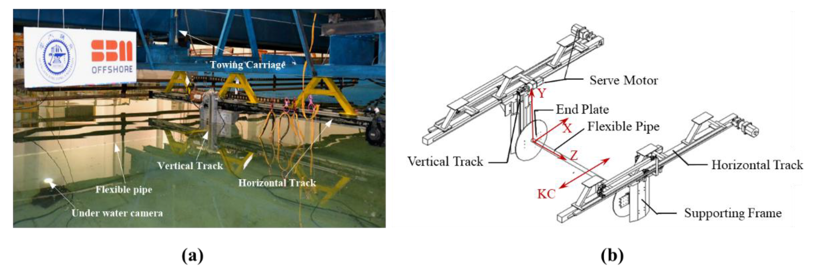
2.1. Experimental Setup

To simulate an equivalent oscillatory flow, the same test apparatus made by Fu et al. (2014) [35] was adopted and forced a flexible pipe to oscillate in harmonic motions under various combinations of amplitudes and periods in an ocean basin at Shanghai Jiao Tong University. The whole experimental apparatus mounted under the bottom of the towing carriage primarily contains two horizontal and vertical tracks as shown in Figure 1. Two force sensors are placed at two ends of the pipe model through universal joints. A pretension force of 500 N was applied to the flexible pipe by a tensioner, which was connected to the force sensor and fixed to a side of the vertical tracks. The vertical track was used to adjust submerged depth of the model, and the horizontal tracks drove the pipe to oscillate. Two endplates were used to reduce the disturbance of the supporting frame to the equivalent oscillatory flow field.

The flexible pipe was made up of a polypropylene random pipe that is filled with copper cable inside. Silicone gel was placed between different layers to prevent relative slippage. The details of the flexible pipe are listed in

Table 2. Parameters of the flexible pipe model.

Item	Value
Model length L (m)	4
Outer diameter D (mm)	29
Mass of flexible pipe in the air $\overline{m}$ (kg/m)	1.529
Mass ratio of flexible pipe (m*)	2.3
Bending stiffness EI (N·m2)	46.43
Tensile stiffness EA (N)	1.528 × 106
Pre-tension FT0 (N)	500
Damping ratio ζ	2.53%
Calculated first natural frequency f10 in still water (Hz)	1.90
Calculated second natural frequency f20 in still water (Hz)	4.08

. The bending stiffness is 46.433 N·m² and the damping ratio is 2.53%. The 1st and 2nd order eigen frequency of the flexible pipe in still water can be calculated by which can be calculated by Equation (1).

$$f_{n0}=\frac{n}{2L}\sqrt{\frac{F_{T_0}}{m}+\frac{n^2{\pi }^2}{L^2}\cdot \frac{EI}{m}},m=\overline{m}+\frac{1}{4}\pi D^2\rho C_m,$$

(1)

where F_T0 is the pretension force of 500 N, m is the mass of bare pipe per unit length in still water, and L and D are the length and diameter of flexible pipe, respectively. EI is the bending stiffness of the pipe, and ρ is the density of water, ρ = 1000 kg/m³. The added mass coefficient is chosen as C_m = 1.0. Notably, the added mass may deviate from the value of 1.0 in still water, and the forced oscillation periods will change with the KC number at the same maximum reduced velocity. n is the mode number.

Four groups of Fiber Bragg Grating (FBG) strain sensors were installed on the surface of the flexible pipe to measure the strain responses in both the CF and IL directions. Each of the FBG groups (CF_a, CF_c, IL_b and IL_d) had ten measurement points along the pipe separated by 0.36 m, as shown in the schematic diagram in Figure 2.

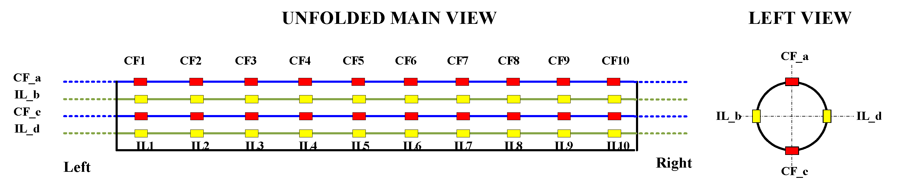
2.2. Test Arrangement

For convenience of description, the coordinate system is defined as O-XYZ as shown in Figure 1b. The origin is at the end point of the test model. The Z axis is along the length of pipe. The X axis is the in-line flow direction, and the Y axis is the cross-flow direction. In our model test, the instantaneous displacement X(t) and velocity U(t) of forced harmonic motions in the horizontal direction can be expressed as:

$$X(t)=A_m\sin \left(\frac{2\pi }{T}t\right)$$

(2)

$$U(t)=U_m\cos \left(\frac{2\pi }{T}t\right), U_m=A_m\frac{2\pi }{T}$$

(3)

where A_m and T are oscillation amplitude and period, respectively. U_m is the amplitude of the forced motion velocity.

The key parameters determining the VIV features of the flexible pipe under oscillatory flow are the KC and maximum reduced velocity V_R [37]. The KC number is defined as follows in Equation (4).

$$KC=\frac{2\pi \cdot A_m}{D},$$

(4)

In our experiments, the excited dominant mode is designed to be the 1st and 2nd modes. The corresponding maximum reduced velocity V_R1 and V_R2 is expressed as Equations (5) and (6), respectively.

$$V_{R1}=\frac{2\pi \cdot A_m}{T\cdot f_{10}\cdot D}$$

(5)

$$V_{R2}=\frac{2\pi \cdot A_m}{T\cdot f_{20}\cdot D}$$

(6)

To investigate the VIV performance of the flexible pipe under higher modes in an oscillatory flow, the test cases are divided into two groups with different designed vibration modes under the same maximum reduced velocities. The comparison group and the group with higher modes used the f₁₀ (f₁₀ = 1.90Hz) and f₂₀ (f₂₀ = 4.08Hz) to design test cases, respectively. All test cases are listed in

Table 3. Test Matrix.

Case No.	VR	Mode	Am(m)	KC	Remax
1–8	5.6	1st	0.10–0.76	22–165	7860
9–15	5.2	2nd	0.22–0.76	48–165	15,696

. The maximum reduced velocities are approximately 5.5. The KC number ranges from 22 to 160. The corresponding maximum Reynolds number (Re_max) is also listed in this table, which can be calculated by Equation (7):

$${\mathrm{Re}}_{\max }=\frac{U_{m}D}{\upsilon },$$

(7)

where U_m is the forced motion velocity amplitude, and υ is the kinematic viscosity coefficient. In our experiment, the ambient temperature is maintained near 15 °C, and υ is, therefore, approximately 1.14 × 10⁻⁶ m² s⁻¹.

3. Data Analysis Procedures

3.1. Preprocessing

In the model test, the measured strain in both the IL and CF directions included three components: the initial axial strain caused by pretension, the varying axial strain caused by varying tension, and the bending strain resulted from hydrodynamic forces. Therefore, the pure VIV strain at position z, ε_CF(z,t), can be calculated by:

$${\epsilon }_{CF}(z,t)=\left[{\epsilon }_{CF\_a}(z,t)-{\epsilon }_{CF\_c}(z,t)\right]/2$$

(8)

where ε_{CF_a}(z,t) and ε_{CF_c}(z,t) are the original strain time histories at position z sampled by the CF_a and CF_c measurement points, respectively.

At the same time, the bending strain ε_IL(z,t) in the IL direction can be calculated by Equation (9).

$${\epsilon }_{IL}(z,t)=\left[{\epsilon }_{IL\_b}(z,t)-{\epsilon }_{IL\_d}(z,t)\right]/2$$

(9)

where ε_{IL_b}(z,t) and ε_{IL_d}(z,t) are the original strain time histories at position z sampled by the IL_b and IL_d measurement points, respectively.

Then, a band-pass filter was utilized to eliminate the higher frequency noise in the IL direction and to remove corresponding higher frequency noise and effects of pendulum motion caused by forced motion in the CF direction. The cutoff frequencies of the band-pass filter were 0 Hz and 15 Hz for the IL direction and 2.5fo (fo is the forced oscillation frequency) and 15 Hz for the CF direction.

3.2. Displacement Reconstruction

The displacement reconstruction method is a basic tool for the VIV study [15,21,38]. According to the Euler–Bernoulli beam theory, the VIV displacement response of a flexible pipe under an external load can be expressed as the sum of the modal shapes multiplied by the generalized coordinate values at each step. Taking the response in the CF direction as an example, the VIV displacement response y(z,t) can be expressed as:

$$y(z,t)={\displaystyle \sum _{i=1}^n{p}_i(t){\phi }_i(z), z\in [0,L]}$$

(10)

where p_i(t) is the ith generalized coordinate displacement value at time t, and φ_i(z) is the displacement at position z in the ith modal shape.

Based on an assumption of small deformation, the curvature κ(z,t) can be expressed as:

$$\kappa (z,t)=\frac{{\partial }^{2}y(z,t)}{\partial z^2}={\displaystyle \sum _{i=1}^n{p}_i(t){\phi }_i^{″}(z), z\in [0,L]}$$

(11)

where ${\phi }_i^{″}$ is the ith modal shape of the curvature. According to the geometric relationship between the curvature and strain, the strain can be calculated by:

$$\epsilon (z,t)=\kappa (z,t)R=R{\displaystyle \sum _{i=1}^n{p}_i(t){\phi }_i^{″}(z), z\in [0,L]}$$

(12)

where R denotes the radius of the flexible pipe model at position z.

In the flexible pipe model, the modal shape of the displacement is sinusoidal since the two ends of the beam are hinged boundary using universal joints, and thus can be expressed as:

$${\phi }_i(z)=\sin \frac{i\pi z}{L}, i=1,2...$$

(13)

From Equation (11), the modal shape of the curvature is also sinusoidal. After obtaining the modal shapes of the displacement and curvature, the generalized coordinates can be obtained from Equation (12). Then, the VIV displacement response in the CF direction can be calculated by Equation (10). Using the same method, the displacement response of the IL direction can also be obtained.

3.3. Time–Frequency Analysis

In an oscillatory flow, the shedding frequency changes with the periodic oscillation velocity of the model, which can be written as:

$$f_{st}(t)=\frac{St\cdot \left|U(t)\right|}{D}$$

(14)

where St refers to the Strouhal number (typically, St = 0.2), and f_st is the vortex shedding frequency.

Under the effect of a periodically varying shedding frequency, the VIV characteristics in the CF direction vary with time. This time-varying feature has been reported to be the major difference between the VIV in steady flow and that in an oscillatory flow [35]. To investigate this time-varying feature under higher modes, the wavelet transform is introduced to analyze the time–frequency distribution of VIV in an oscillatory flow. The continuous wavelet transform equation is expressed as:

$$W{T}_f(a,\tau )=\langle f\left(t),{\psi }_{a,\tau }\right(t)\rangle =a^{-1/2}{\displaystyle {\int }_{-\infty }^{+\infty }f\left(t\right)}\psi *(\frac{t-\tau }{a})dt$$

(15)

where WT_f(a,τ) is the coefficient of the time-domain signal f(t) after the wavelet transform representing the frequency variation at that time scale, the parameter a is the scale factor, τ is the shift factor, and ψ(t) is the mother wavelet. In this paper, the Morlet wavelet equation is employed as the mother wavelet, and this wavelet can be defined as:

$$\psi (t{)=\mathrm{Ce}}^{-t^2/2}\cos (5t)$$

(16)

where C is the wavelet transform coefficient.

4. Results and Discussions

4.1. Spatial and Temporal Distributions of VIV Responses

Based on the method of displacement reconstruction described in Section 3.2, the displacement modal weights and the displacement response can be obtained. Figure 3 shows the root mean square (RMS) values of the displacement weights (p_rms) in the CF direction in the cases of KC = 56 and 121 under V_R2 = 5.2. It shows that the second mode dominates the VIV response in all cases. The dominant vibration mode is expected as designed. Moreover, the first mode vibration is also obvious, except for second order modes, especially for larger KC numbers (KC = 121). This indicates that the multimode will participate in vibrations.

Figure 4 shows the corresponding RMS value distribution of the displacement response along the flexible pipe in both the CF and IL directions. The blue solid line and the red dashed line represent the displacement response for KC = 56 and 121 under V_R2 = 5.2, respectively. Figure 4a shows that the RMS value of the VIV response (Y_RMS) for KC = 121 is smaller than that for KC = 56, except for the node of the second mode shape (Z/L = 0.5). Meanwhile, the value in the IL direction (X_RMS) for KC = 121 is correspondingly less than that for KC = 56 as shown in Figure 4b. This means that the drag force acting on the flexible pipe in the IL direction for KC = 121 is weaker than that for KC = 56. The results are consistent with the belief that VIV will enlarge the incoming flow area and increase drag in the IL direction [17,18].

To verify the displacement reconstruction method, the strain was recalculated based on the reconstructed displacement response. Through Equation (12), the curvature can be obtained by the second order difference of the displacement shape multiplying the generalized coordinate displacement value. Then, the strain values are further recalculated by Equation (13). Figure 5 and Figure 6 illustrate the time history of measured and calculated strain in both the CF and IL direction for KC = 56 and 121 under V_R2 = 5.2, respectively. The blue solid line and red dashed line respectively represent measured and calculated strains. Figure 7 presents the distribution of root mean squares of measured and calculated strains along the flexible pipe in both the CF and IL directions in the case of KC = 56 and 121 under V_R2 = 5.2. The blue circles and the red dashed lines represent the measured and calculated values, respectively. It reveals that these calculated values are in good agreement with the measured one. This consistency demonstrates the validity of the displacement reconstruction method for the flexible pipe in an oscillatory flow.

In oscillatory flows, the VIV responses have distinctive time-varying features [35,38,39]. Figure 8 and Figure 9 show the spatial and temporal distribution of the VIV response for KC = 56 and 121 under V_R2 = 5.2, respectively. Each figure has two subfigures: Subfigure (a) is the time history of forced motion velocity, and Subfigure (b) presents spatial–temporal distribution of VIV response. Under a smaller KC number (KC = 56), the displacement response is always dominated by the second mode over time. Steady standing waves can be clearly seen in the whole forced motion as shown in Figure 8b. Different from the results of KC = 56, the first mode and the second mode alternately dominate the VIV response in the case of KC = 121, as shown in Figure 9b. The travelling wave can be observed in the transition region of two modes. The standing wave occurs in the dominated region of the second mode. Thus, VIV under higher modes has the characteristic of time-sharing dominance for each mode for larger KC number. The reason for this can be attributed to the fact that the vortex shedding does not immediately change with forced motion velocity altering [40]. Under KC = 56, the oscillating period is shorter, and the vortex shedding causing the second mode vibration will cover it, resulting in the first mode vibration. As the KC number increases and the correspondingly oscillating period becomes longer, the above effects gradually weaken. Time-sharing of the two modes appears in the case of a larger KC number. More insightful experiments and Computational Fluid Dynamics (CFD) simulations will be carried out in the near future work to further investigate this interesting phenomenon.

4.2. Time-Varying Features of VIV Responses

To further reveal the VIV response features under the higher mode (second mode), the VIV responses near the antinode of second modal shape (Z/L = 0.3) were selected for investigation. Figures 11 and 13 respectively present the time history of the VIV response and time–frequency distributions at Z/L = 0.3 for KC = 56 and 121 under V_R2 = 5.2. Figures 10 and 12 present the corresponding results at Z/L = 0.5 for KC = 56 and 121 under V_R1 = 5.6. Each figure above has four subfigures. Subfigure (a) shows the time history of the forced motion velocity. Subfigure (b) is the time history of VIV displacement response. Subfigure (c) shows the wavelet analysis of the VIV displacement response. The depth of the color indicates the concentration level of the VIV response components. Subfigure (d) indicates the calculated time-varying shedding frequency (f_st), time varying natural frequency (f₁, f₂), and VIV response dominant frequency (f_domi). The black dashed line and purple solid line, respectively, represents VIV response dominant frequency and vortex shedding frequency. The blue dot dashed line and red dot line are the first- and second-order eigen frequency, respectively. Different from Equation (1), f₁, f₂ here considered the measured time-varying tension F_T(t), which is calculated by:

$$f_n(t)=\frac{n}{2L}\sqrt{\frac{F_T(t)}{m}+\frac{n^2{\pi }^2}{L^2}·\frac{EI}{m}}, m=\overline{m}+\frac{1}{4}\pi D^2\rho C_m$$

(17)

while we still assumed the added mass coefficient C_m to be equal to 1 the same as Equation (1).

Under smaller KC number (KC = 56), similar relatively mild amplitude modulation was seen in both Figure 10b and Figure 11b. The maximum VIV response of the flexible pipe can be reached 0.65 D and 0.74 D for V_R1 = 5.6 and V_R2 = 5.2, respectively. The VIV response dominant frequencies are respectively always lock-in the first and second natural frequency as presented in Figure 10d and Figure 11d. Although the vortex shedding frequency varies with time, the dominant frequency is always near the natural eigen frequency of the dominant mode for smaller KC number. There is no mode transition phenomenon in case of smaller KC number under higher mode. This is a distinctive feature of VIV response of flexible under higher mode in an oscillatory flow under smaller KC number.

As KC number increases to 121, amplitude modulation became stronger as shown in Figure 12b and Figure 13b. When V_R1 = 5.6, the VIV developing process including building up, lock-in and dying out can be clearly witnessed in Figure 12b, which were also found by Fu et al. (2014) [35]. However, these three phases cannot be directly seen in Figure 13b and the VIV response was more disordered when V_R2 = 5.2 and KC = 121. These differences are caused by co-participation and intermittent dominance of multiple modes under higher mode vibration for larger KC number. Figure 14 gives the time histories of the first two modal weights. The cyan dashed lines were the envelope of response obtained by the Hilbert transform. The similar VIV development process under V_R1 = 5.6 can be easily found in the second modal weight under V_R2 = 5.2 as shown in Figure 14d, while it is difficult to identify this process in the first modal weight as shown in Figure 14c. Thus, the secondary vibration modes confuse the development process of the dominant vibration mode and lead to more chaotic features of VIV.

In the oscillatory flow, the forced motion contains continuous acceleration and deceleration phases. The second VIV modal response in acceleration and deceleration stages has an obvious asymmetrical characteristic as shown in Figure 14d. The amplitude value in the acceleration phase at half a maximum forced motion velocity (I, III, V) was nearly 0.10 D, while approximately 0.25 D in deceleration phase at points (II, IV, VI). The latter response in the second modal space is larger than the former one. This is termed as “hysteresis” [35]. Different from the VIV response dominated by the first mode, the interesting hysteresis phenomenon did not appear in the total VIV displacement or the first modal response under the higher vibration mode for the larger KC number. The “hysteresis” only occurs in the dominant response modal space.

Beyond that, the “mode transition” and the alternate mode lock-in are prominent for the larger KC number (KC = 121) under V_R2 = 5.2 as presented in Figure 13c,d. This is absent in the VIV response dominant by only the first vibration mode as illustrated in Figure 12c,d, and it is also not found under the smaller KC number (KC = 56) under the same maximum reduced velocity of the higher mode as presented in Figure 11c,d. With vortex shedding frequency increasing from zero to the maximum value, the dominant frequency first locked in the first natural frequency of approximately 1.95 Hz and jumped to lock in at the second natural frequency of nearly 3.8 Hz. When the vortex shedding frequency reached around the second natural frequency in the acceleration phase, the response dominant frequency started jumping from the first mode to the second mode. However, the frequency turning points of the lock-in mode decreased from the second to the first mode occurred when the vortex shedding frequency fell between 0 Hz to the first natural frequency and displayed some uncertainties. Thus, the higher mode locking establishment frequency and unlocking frequency are significantly different, which can also be attributed to the lag of vortex shedding as previously mentioned. Vortex shedding does not change immediately with forced motion velocity altering, and the locking time of the higher mode vibration becomes longer, accordingly. Although the interesting phenomenon of “mode transition” and the alternate mode were revealed above, the prediction of the critical transition frequency awaits to be determined by more extensive experiments and studies in the future.

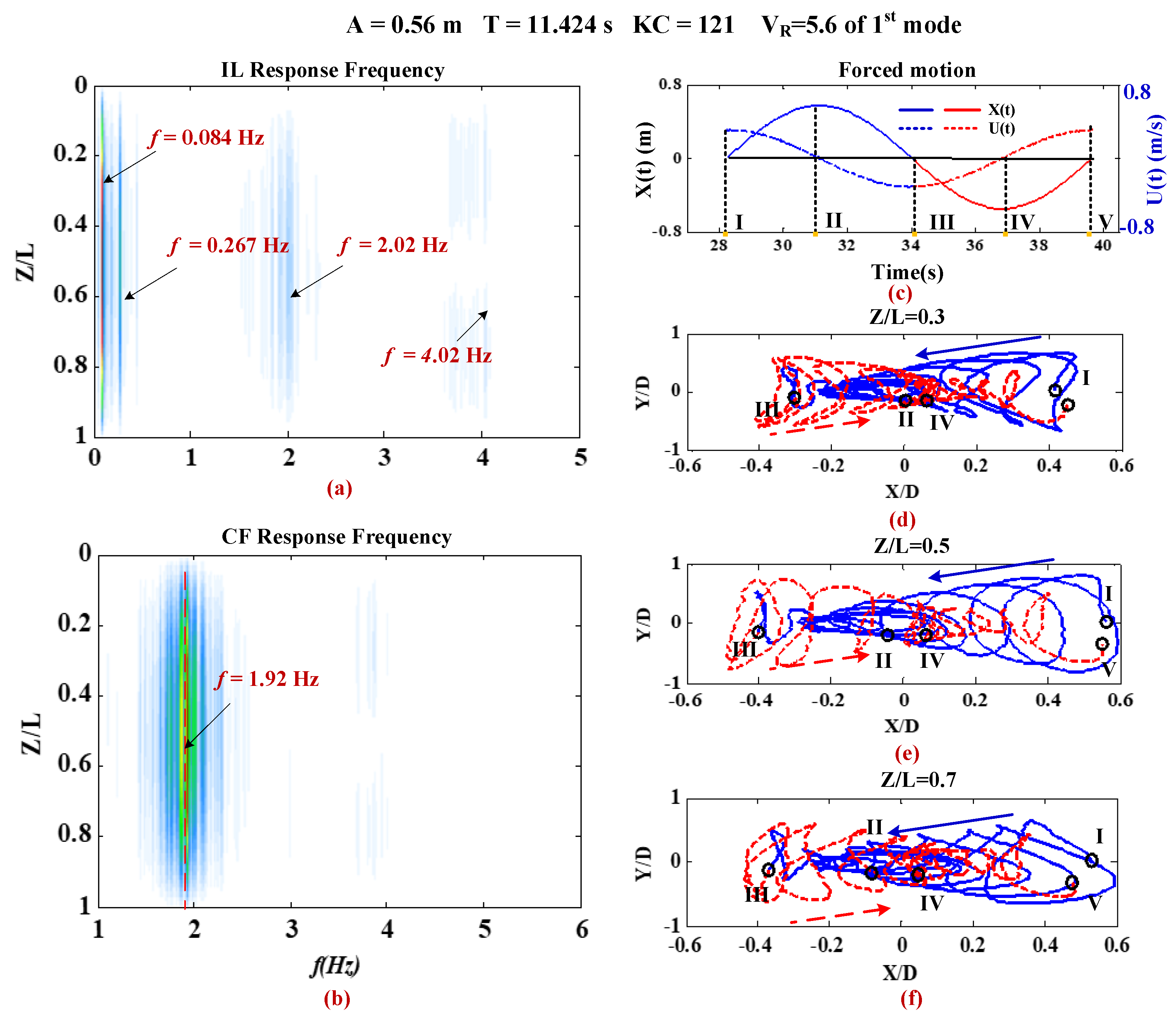
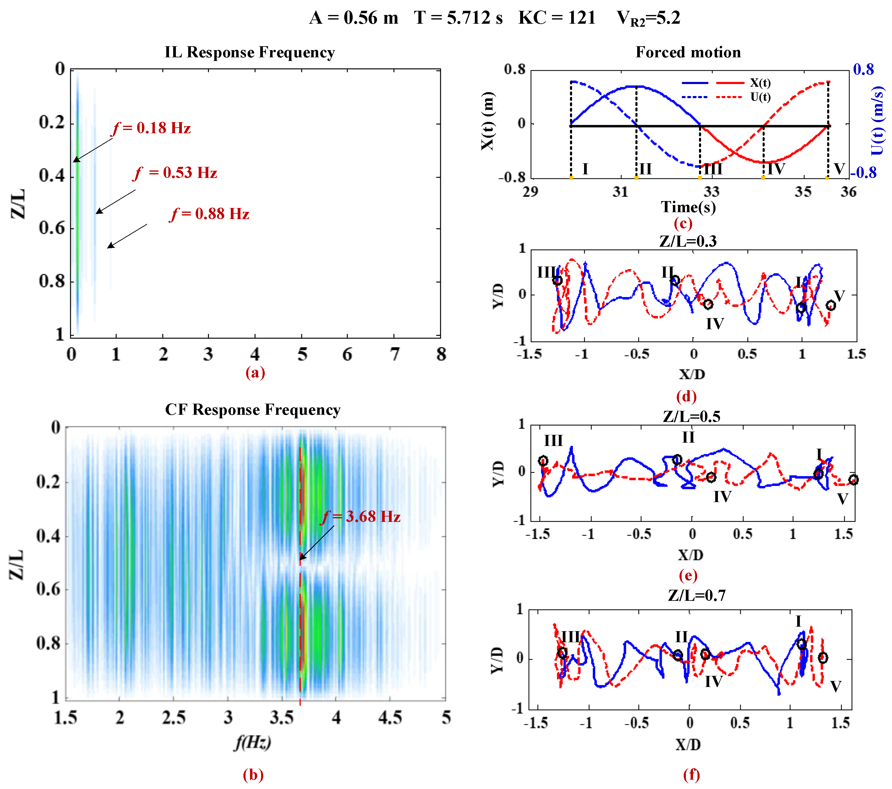
4.3. Response Frequencies and Trajectories

For the convenience of investigating performances of response trajectory and frequency under higher mode vibrations, Figure 15 and Figure 17 first show the spatial distribution of response frequency in the IL and CF directions and the cross-section displacement trajectories at Z/L = 0.3, 0.5, 0.7 when KC = 56 and 121 under V_R1 = 5.6 in one oscillation cycle, respectively, which is processed by MATLAB software. Figure 16 and Figure 18 present the above under V_R2 = 5.2. The dominant frequency of VIV response in both the IL and CF direction are summarized in

Table 4. Summary of dominant frequency of VIV for different test cases.

VR	KC	Dominant Mode	Forced Motion Frequency (fo)	Dominant Frequency of VIV	Direction
VR1 = 5.6	56	1st	0.188 Hz	0.565 Hz (3fo)	IL
VR1 = 5.6	56	1st	0.188 Hz	1.938 Hz (10fo)	CF
VR2 = 5.2	56	2nd	0.38 Hz	1.290 Hz (3fo)	IL
VR2 = 5.2	56	2nd	0.38 Hz	3.785 Hz (10fo)	CF
VR1 = 5.6	121	1st	0.084 Hz	0.267 Hz (3fo)	IL
VR1 = 5.6	121	1st	0.084 Hz	1.920 Hz (22fo)	CF
VR2 = 5.2	121	2nd	0.18 Hz	0.530 Hz (3fo)	IL
VR2 = 5.2	121	2nd	0.18 Hz	3.680 Hz (21fo)	CF

. Under the smaller KC number (KC = 56) with V_R1 = 5.6, Figure 15a shows the dominant response frequency in the IL direction, the same as expected for the forced motion frequency at f = 0.188 Hz (f_o). The secondary contribution from the VIV response in the IL direction is dominated by f = 0.565 Hz (3 f_o). The VIV response in the CF direction is dominated by f = 1.907 Hz (10 f_o) as shown in Figure 15b. Comparing two spatial distributions of VIV response frequencies, the corresponding twice VIV dominant frequency in the CF direction is inconspicuously observed in Figure 15a. There is no clear relationship where the VIV dominant frequency in the IL direction is twice of that in the CF direction. This is inconsistent with the results of the frequency relationship found in steady flow reported by Blevins and Saunders (1977) [1].

With the design vibration mode increasing to 2 for KC = 56, removing the response corresponding to the forced motion frequency (f_o = 0.38 Hz) in the IL direction, the VIV response in the IL direction is dominated by f = 1.129 Hz (3f_o) and participated in an insignificant frequency contributor f = 1.892 Hz (5f_o) as shown in Figure 16a. The VIV response frequency in the CF direction is dominated by f = 3.785 Hz (10f_o) as shown in Figure 16b. f = 0.322 Hz (9f_o), and f = 4.548 Hz (12f_o) can also be seen, but is not obvious. The twice relationship of the VIV response dominant frequency between the CF and IL directions is also not easy to find under the higher mode in the case of a smaller KC number. Under the larger KC number (KC = 121), the frequency results are similar to those in the case with smaller KC numbers. The VIV response dominant frequency in the case of KC = 121 and V_R1 = 5.6 is f = 0.267 Hz (3f_o) and f = 1.92Hz (22f_o) for the IL and CF direction as shown in Figure 17a,b, respectively. The frequencies f = 0.53 Hz (3f_o) and f = 3.68 Hz (21f_o), respectively, dominates the VIV response in the IL and CF directions with KC = 121 under V_R2 = 5.2 as presented in Figure 18a,b. Thus, it suggests that the traditional VIV response frequency relationship between the IL and CF directions cannot be directly used to predict the VIV response in an oscillatory flow. Beyond that, an interesting phenomenon is witnessed in that the dominant response frequency and other secondary frequencies all maintain the multiple relationship with the frequency of the forced motion. Similar phenomena are also found from stationary rigid cylinder experiments in an oscillatory flow [37]. Moreover, the VIV responses in the IL direction are always coincidentally dominated by 3f_o. This provides a possible reference for a VIV prediction in the near future.

Displacement trajectories can directly reveal the whole response process of a flexible pipe in an oscillatory flow. We firstly select five typical time points (I, II, III, IV, and V) to mark and to help us to describe the features of displacement trajectories at different acceleration or deceleration phases as shown in Subfigure (c) of Figure 15, Figure 16, Figure 17 and Figure 18. The necessary comparisons of displacement trajectories mainly include the following two items:

(1) The performance of trajectories changes before and after reverse motion such as those in the stages I→II and II→III, III→IV, and IV→V. Under the smaller KC number of V_R1 = 5.6, taking one pair stages (I→II and II→III) in half an oscillation cycle for observation, the trajectories from time I to II are not symmetrical to those from time II to III as shown in Figure 15d–f. The response in phase (I→II) is slightly larger than that in phase (II→III), which indicates that the response was suppressed in the reverse motion stages. The same results can be also witnessed in phases (III→IV) and (IV→V) as shown in Figure 15d.

One reason for this asymmetry may be attributed to the vortex shedding interaction, when the cylinder reverses its motion direction and encounters the previously shed vortices [6,36]. The vortex shedding interaction leads to a correspondingly different response before and after the reverse motion. Nevertheless, we cannot rule out the effects of vortex shedding lag. At point I, the forced motion starts to slow down, and stronger shedding vortices catch up with the flexible pipe, resulting in a larger response in the process from I to II. These effects will weaken over time. Thus, the response asymmetry and a larger response of I→II than that of II→III were observed. When the KC number increases to 121 under V_R1 = 5.6, the asymmetric features in phase (I→II) and (II→III) of the trajectory become very apparent, as shown in Figure 17d–f.

With the dominated mode increasing to the second mode, similar results can also be found under the smaller KC number (KC = 56) as shown in Figure 16d–f. However, the aforementioned prominent features are not obvious in the case of the larger KC number (KC = 121) under V_R = 5.2 of the second mode as illustrated in Figure 18d–f. A multifrequency response and a multimode intermittent disrupt the features above.

(2) Differences of trajectory in acceleration and deceleration stages merit study. In the case of the smaller KC number when V_R1 = 5.6, trajectory discrepancies are very obvious between acceleration stage II→III and deceleration stages III→IV as presented in Figure 15d–f. More significant results can be found when KC increases to 121 under V_R1 = 5.6 as shown in Figure 17d–f. Under smaller KC numbers with V_R1 = 5.6, the discrepancies of the cross-section trajectory are mainly derived from the response phase differences between the CF and IL directions, while response amplitude discrepancies contribute to the corresponding differences in trajectory under larger KC numbers with V_R1 = 5.6. Moreover, under the higher mode V_R2 = 5.2, although a distinctively inconsistent trajectory can directly observed in both smaller and larger KC numbers, as shown in Figure 16d–f and Figure 18d–f, respectively, differences of trajectories can be all attributed to response phase differences. The response amplitude difference is slight and is a secondary reason for trajectory discrepancies in the case of VR = 5.2 of the second mode.

Beyond that, under V_R1 = 5.6, the trajectory of the walking “8” and “o” shapes can be observed, especially for the larger KC number (KC = 121) as shown in Figure 17d–f. When the design dominated mode increased to the second mode, the quasi-regular track characteristics like the walking “8” and “o” shapes disappeared without any trace for smaller or larger KC numbers as presented in Figure 16d–f and Figure 18d–f. Furthermore, some differences do exist in the trajectory along the length of the flexible pipe whether the higher order mode is dominated or only the first mode is involved. Subfigures (d–f) of Figure 15, Figure 16, Figure 17 and Figure 18 display this well. It should be emphasized that the response amplitude and the response phase between the IL and CF directions are two essential factors for hydrodynamic force coefficients. The results above indicate that hydrodynamic coefficients before and after the reverse motion, acceleration, and deceleration stages will be different. A different trajectory along the flexible pipe means that a different cross section will have different hydrodynamic coefficients. Thus, hydrodynamic coefficients may display spatial and temporal varying features [39,41,42,43]. Moreover, the trajectory discrepancies between the higher mode dominated and only the first mode involved manifest that hydrodynamic coefficients under a response dominated by a higher mode will have certain novel and complex characteristics that need to be studied in future work.

4.4. General Discussions

Based on this detailed case study, features of the VIV response of a flexible pipe under oscillatory flow with the higher mode dominated are different from that with only the first mode dominated through comparing smaller and larger KC numbers under the same maximum-reduced velocity of different design dominated modes. Under the higher mode with the larger KC number, the mode transition and alternate mode lock-in are prominent. A travelling wave occurs in the mode transition stage and the standing wave appears in the lock-in one. However, the alternate mode lock-in phenomenon cannot occur, and the VIV response is always locked in the dominated mode for the smaller KC number with the higher mode. The standing wave is always seen in the spatial and temporal distributions of the VIV. The travelling wave characteristic is not found in the case of the smaller KC number under the higher mode. Different from only the first mode excited case, VIV processing, including building up, lock-in and dying out, and hysteresis, are clearly witnessed only in the dominated modal space. This indicates that the response of the secondary participate mode does not affect the VIV process or features in the dominated modal space.

The aforementioned detailed features provide us with a basic understanding of the VIV response under the higher mode in the case of different KC numbers. The VIV displacement amplitude of each case should be further summarized. Figure 19 shows the maximum root mean square VIV displacement versus the KC number under different dominated modes. The blue triangle and red circle represent the responses under V_R1 = 5.6 and V_R2 = 5.2, respectively. The decreasing tendency of response amplitude with KC number can be observed under two dominant designed modes. Under the small KC number, the interaction of vortex shedding before and after the reverse forced motion is stronger for the small KC number case, leading to a larger response [36]. In the case of the larger KC number, the maximum value of Y_RMS/D approaches towards a constant value asymptotically as the KC number increases. The value differences of VIV response amplitudes under two dominated modes are not large. This indicates that the effects of higher dominated mode (>2) in an oscillatory flow on VIV response amplitude may be slight.

In Section 4.3, the response frequency and trajectory under different dominated modes in an oscillatory flow are compared. Discrepancies of response trajectories are revealed between different dominated modes and may cause some unknown effects on hydrodynamic force. Future work should emphasize the investigation of hydrodynamic coefficients under higher modes. Moreover, response frequency always maintains a multiple relationship with the frequency of the forced motion whether is dominated by a higher mode or not. The response frequency calculation is an essential issue in VIV prediction. For the VIV of a rigid cylinder in an oscillatory flow, Sumer and Fredsøe (1988) [37] found the integral multiple relationship between the VIV dominant response frequency f_domi in the CF direction and the oscillatory flow frequency f_o. This result is consistent with our observation on the VIV response of the flexible pipe in an oscillatory flow as previously described. It indicates that there are integral vortices shedding for each motion period. These vortex shedding pairs N are defined as:

$$N=\frac{f_{domi}}{f_o}$$

(18)

In a steady flow, the VIV dominant frequency is governed by the Strouhal number (St). The typical value of the St number is found to be approximately 0.2 through the stationary smooth cylinder in a steady flow [1]. To further investigate the effects of dominated modes on the St number and to extract the exact value of the St number, the relationship among the VIV dominant frequency, the number of vortex shedding pairs, the KC number under oscillatory flow, and the Strouhal number can be expressed as follows:

$$\begin{array}{l}\frac{N}{KC}=\frac{f_{domi}}{f_o}\cdot \frac{D{f}_o}{U_m}=\frac{f_{domi}D}{U_m}=St\\ N=St\cdot KC\end{array}$$

(19)

The aforementioned relationship was first introduced to investigate the St number of a smooth rigid cylinder in an oscillatory flow by Sumer and Fredsøe (1988) [37]. However, it can be also applied for the flexible pipe and has been used in the SCR and free-hanging riser model tests [27,33,34]. Through Equation (18), the dominant frequency of all cases is first summarized, and the vortices shedding pairs N are then calculated. The distributions of vortex shedding pairs versus KC numbers are presented in Figure 20. The vortex shedding pairs maintain a good linear relationship with the KC numbers. Based on Equation (19), the values of the St number under V_R1 = 5.6 and V_R2 = 5.2 are 0.18 and 0.174, respectively. These values are slightly lower than the typical value of 0.20, which is consistent with the results reported by Wang et al. (2015) [27]. Comparing St numbers under two different dominated modes in an oscillatory flow, the two values are very close, and the differences can be ignored. Thus, we can infer that the St number is controlled by the maximum reduced velocity and not related with the dominated modes in the CF direction.

Moreover, the dominant frequency of the VIV response in the IL direction is different from that in the CF direction as depicted in Figure 15a, Figure 16a, Figure 17a and Figure 18a. The dominant frequency seems to always be triple the oscillatory flow frequency. Thus, the dominant frequency prediction of the VIV response in the IL direction can be directly calculate by this simple relationship. Although the VIV response dominant frequency in both the IL and CF directions can be preliminarily predicted, the time varying frequency features under larger KC numbers require a critical value to determine whether dominant lock-in frequency jump has occurred.

Future work should conduct a more systematic series of experiments. The lock-in frequency jump between multimode needs a critical value to be further determined. The hydrodynamic coefficients under different excited modes, KC numbers and maximum reduced velocity are also emphasized for future investigation.

5. Conclusions

In this paper, an experimental study on the VIV of a flexible pipe under a higher mode in an oscillatory flow was carried out with a V_R of approximately 5.5 in the case of KC numbers varying from 22 to 165. The dominant excited mode was designed for the first and second modes. The VIV displacement and time-varying frequency are reconstructed and identified through the modal superposition method and wavelet transform, respectively. Compared with only the first mode excited cases, the features of VIV were further investigated. The main conclusions are as follows:

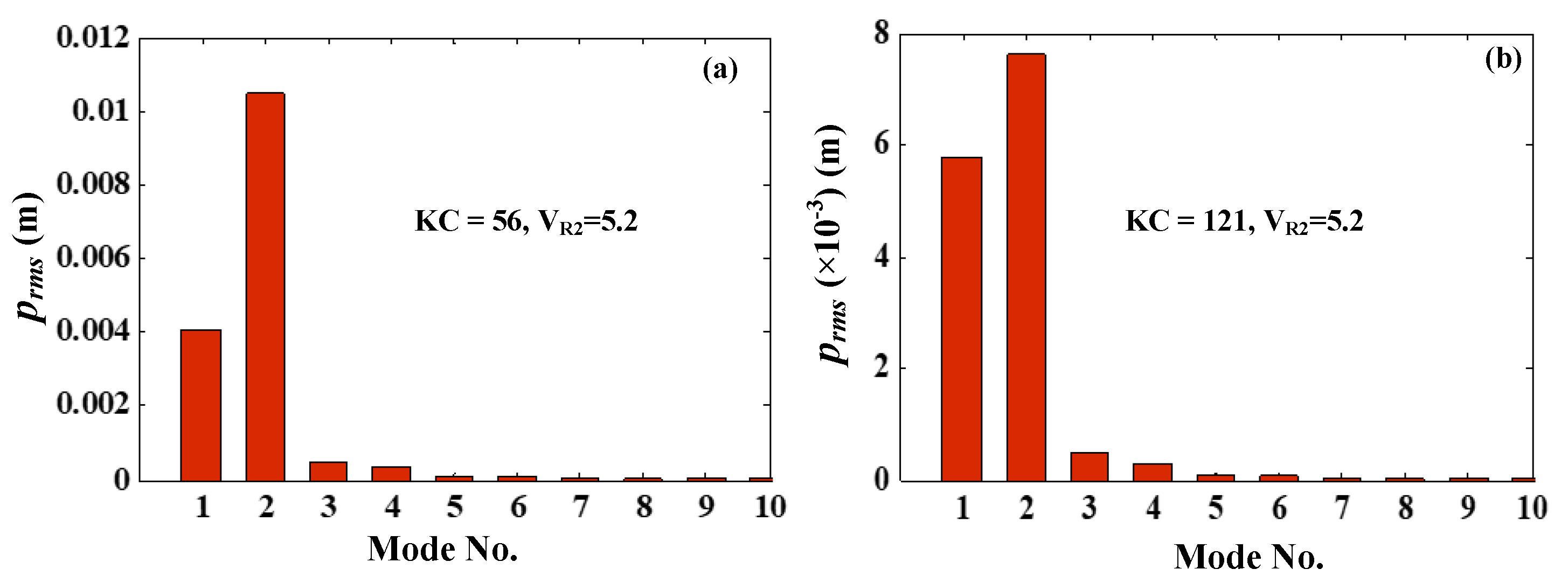
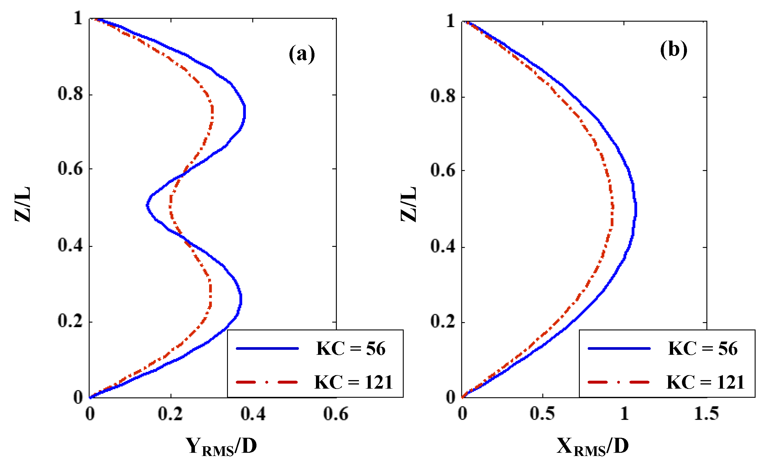
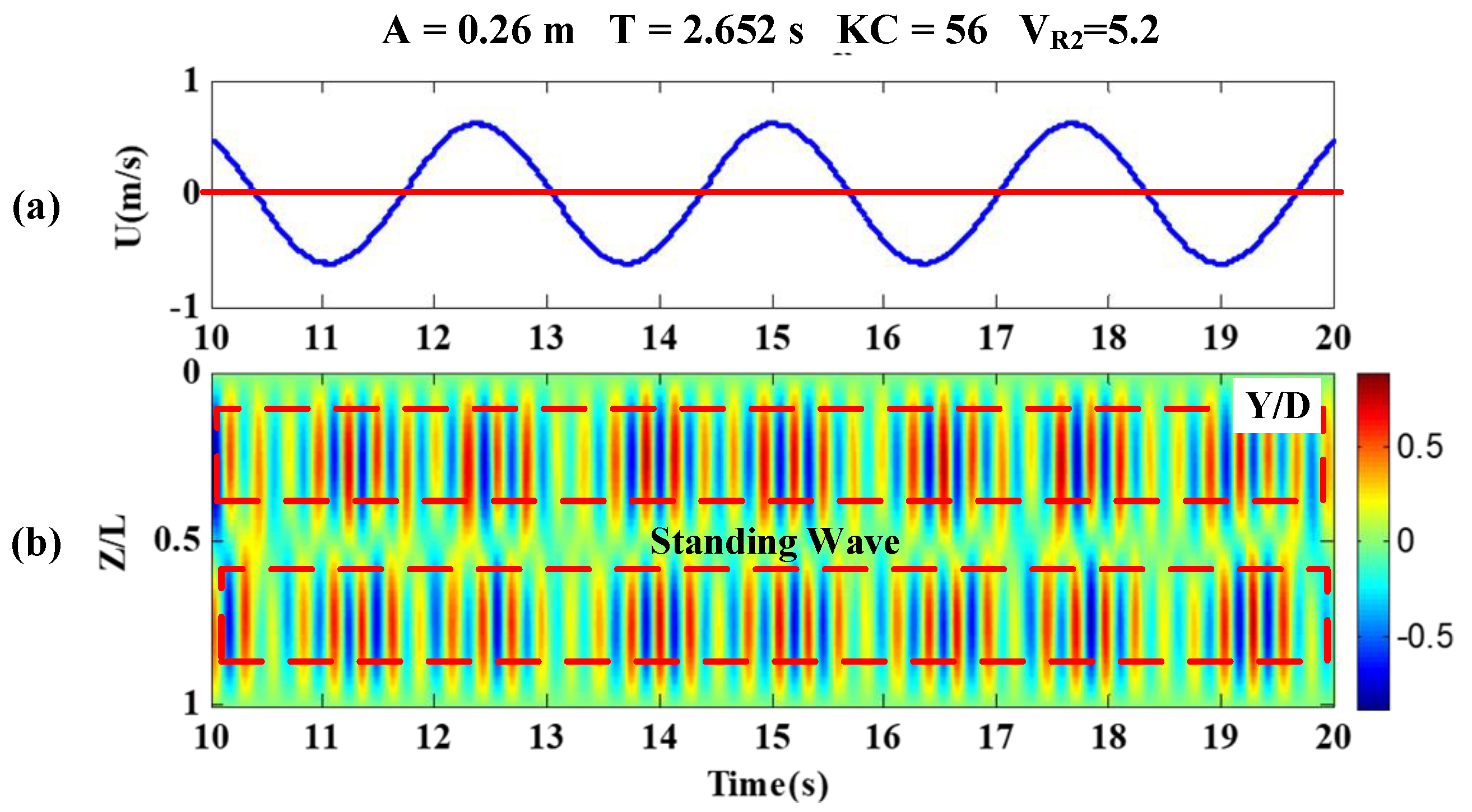
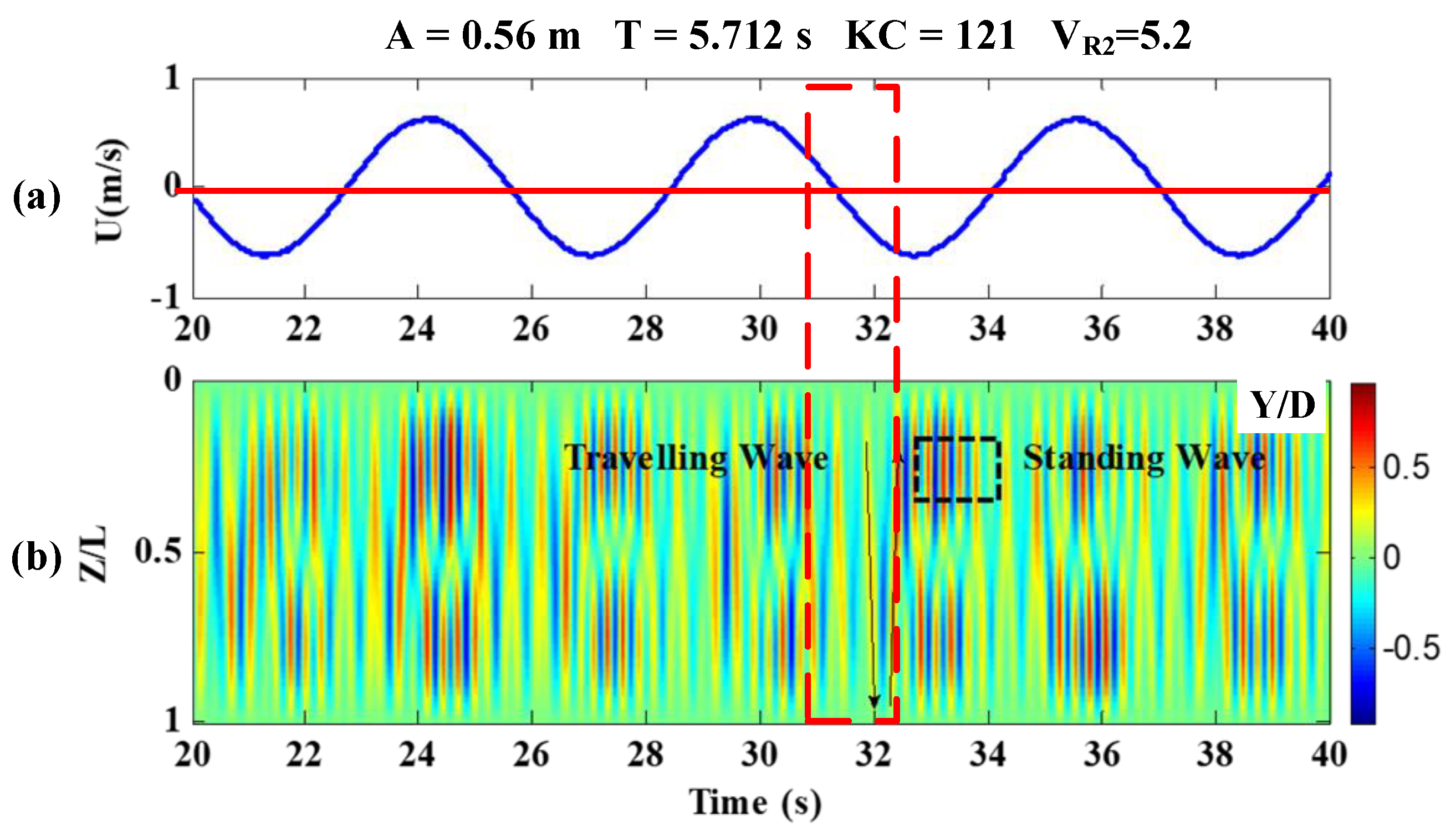
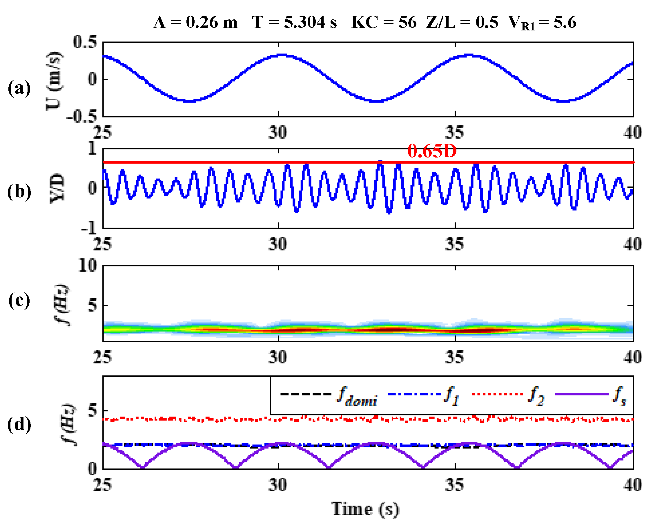
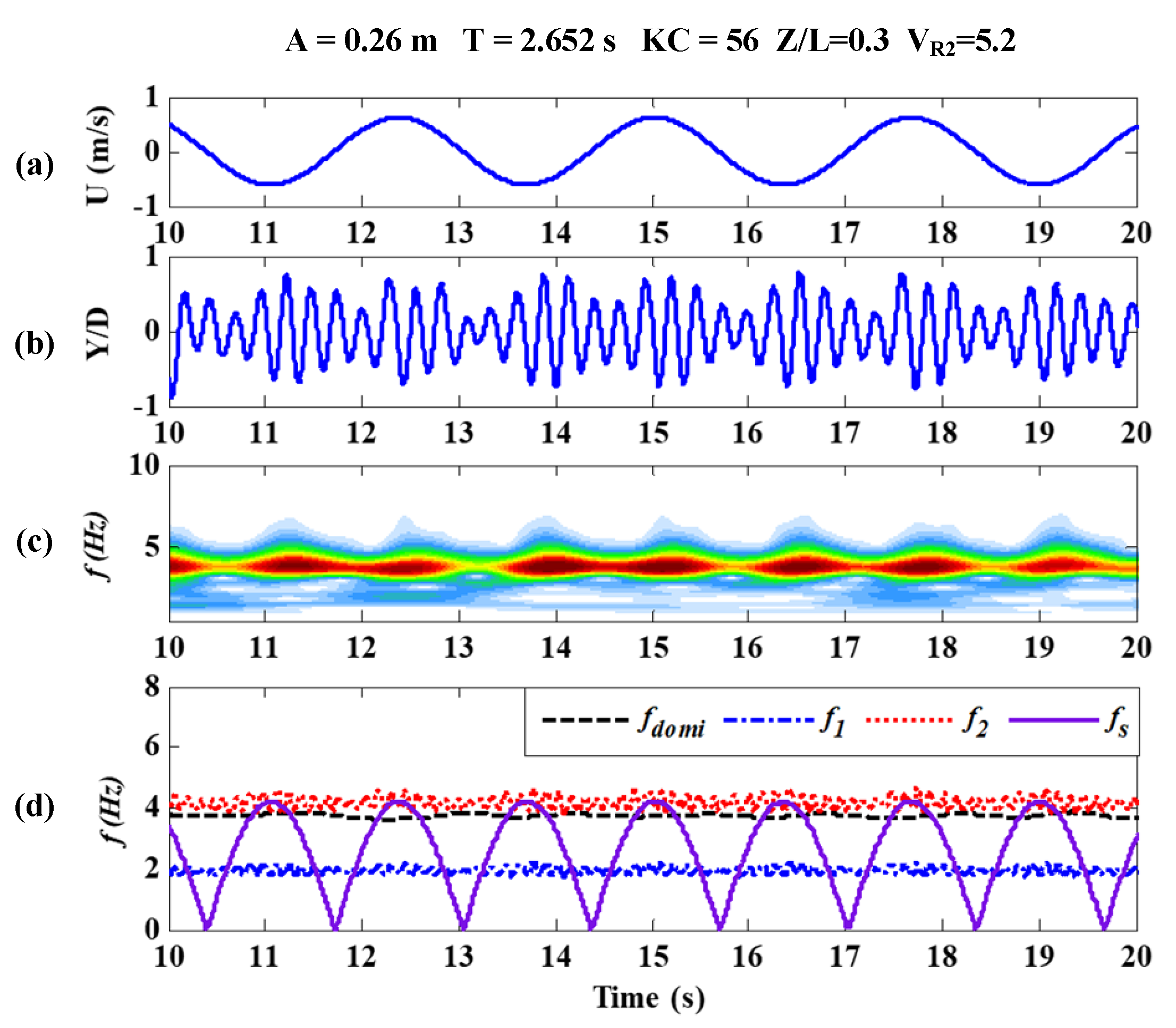
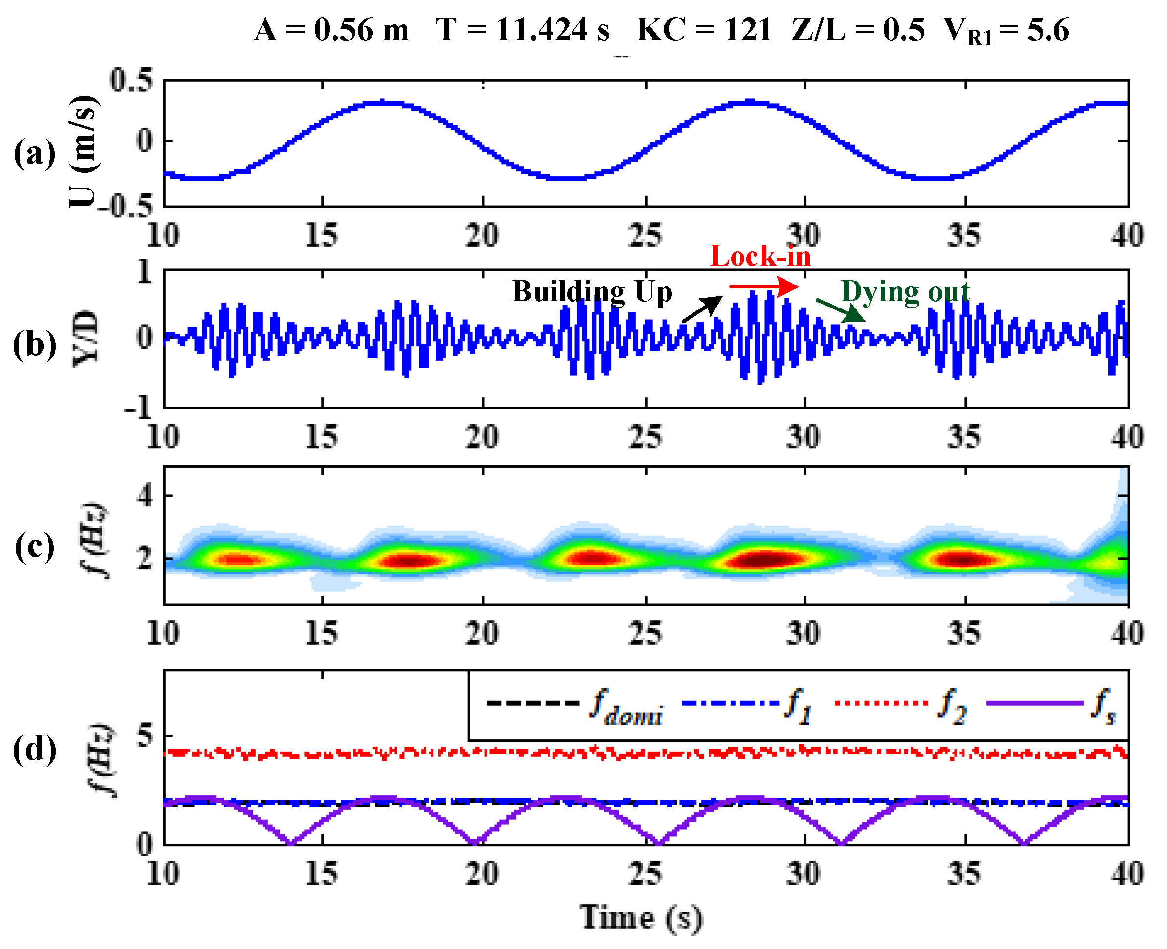
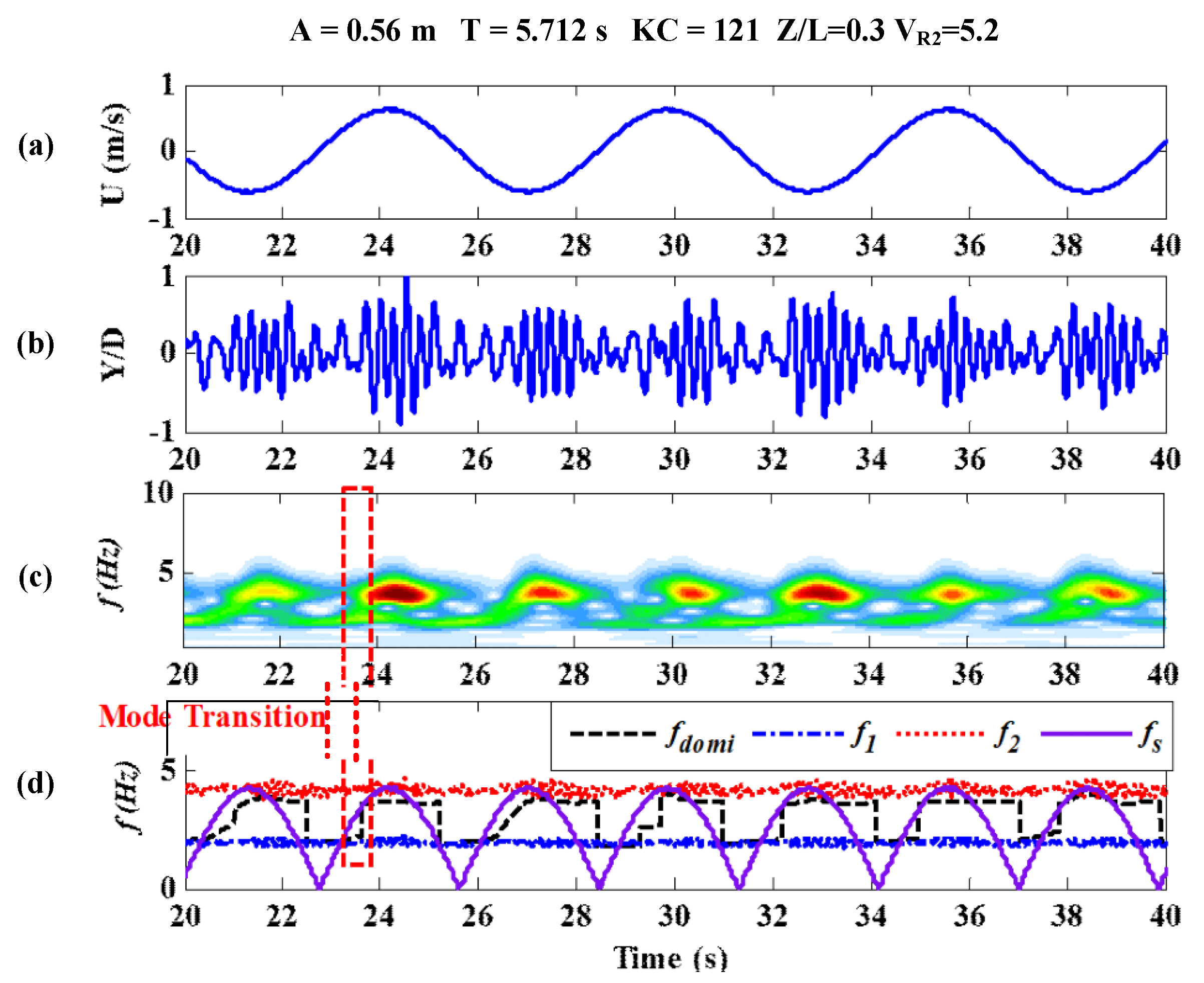
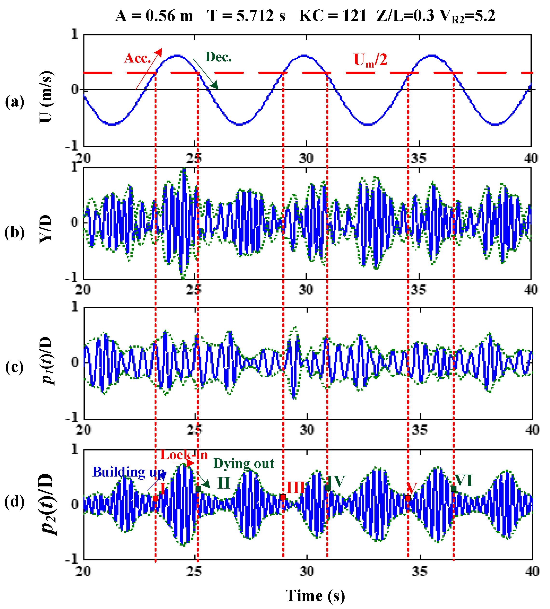
• Under the higher mode, a travelling wave is observed in the mode transition regions for larger KC numbers. An alternate mode lock-in occurs in the case of larger KC numbers, but does not occur for smaller KC ones. A distinctive feature for smaller KC number is that the VIV response of the flexible pipe always locks in the dominant mode.
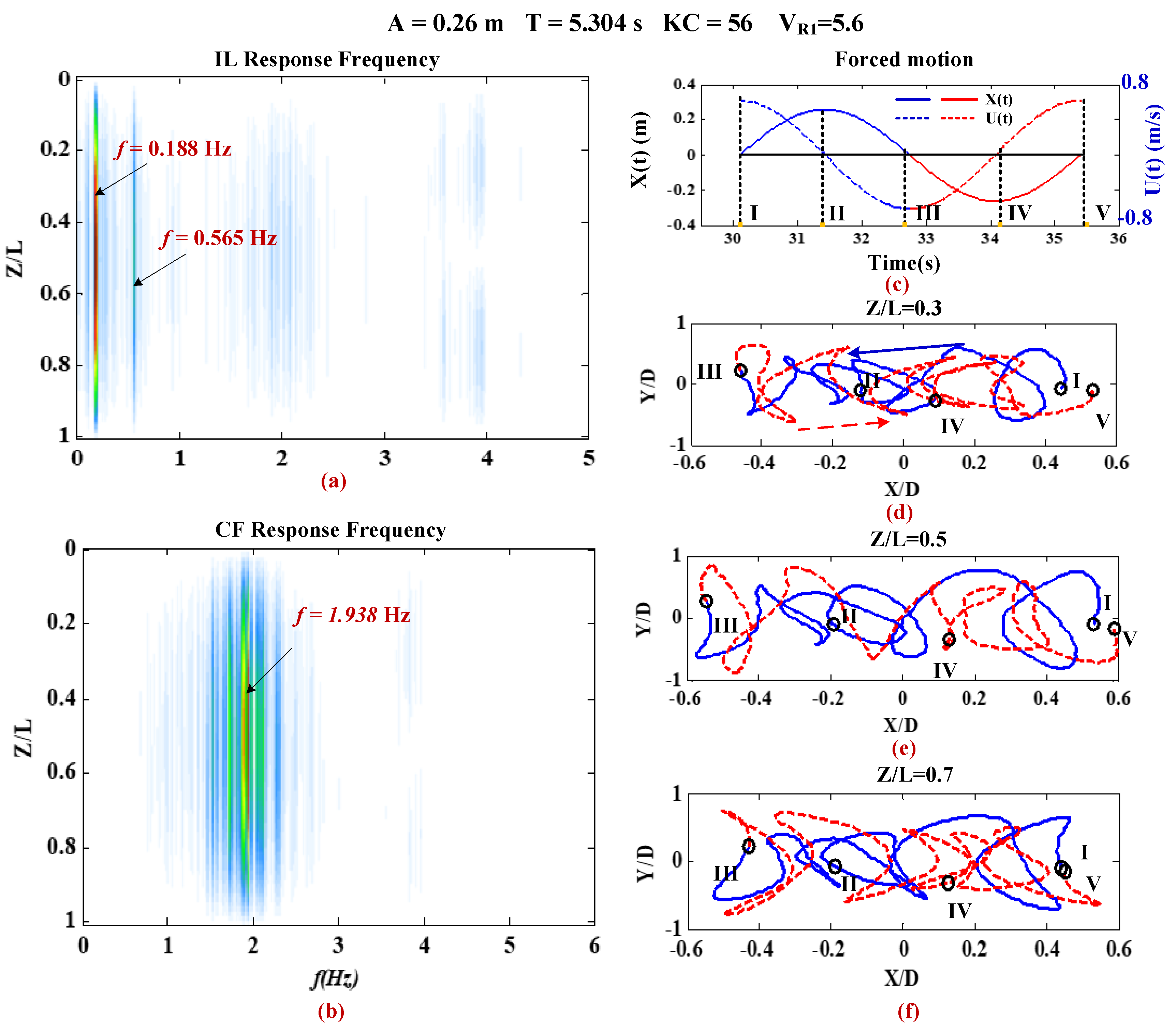
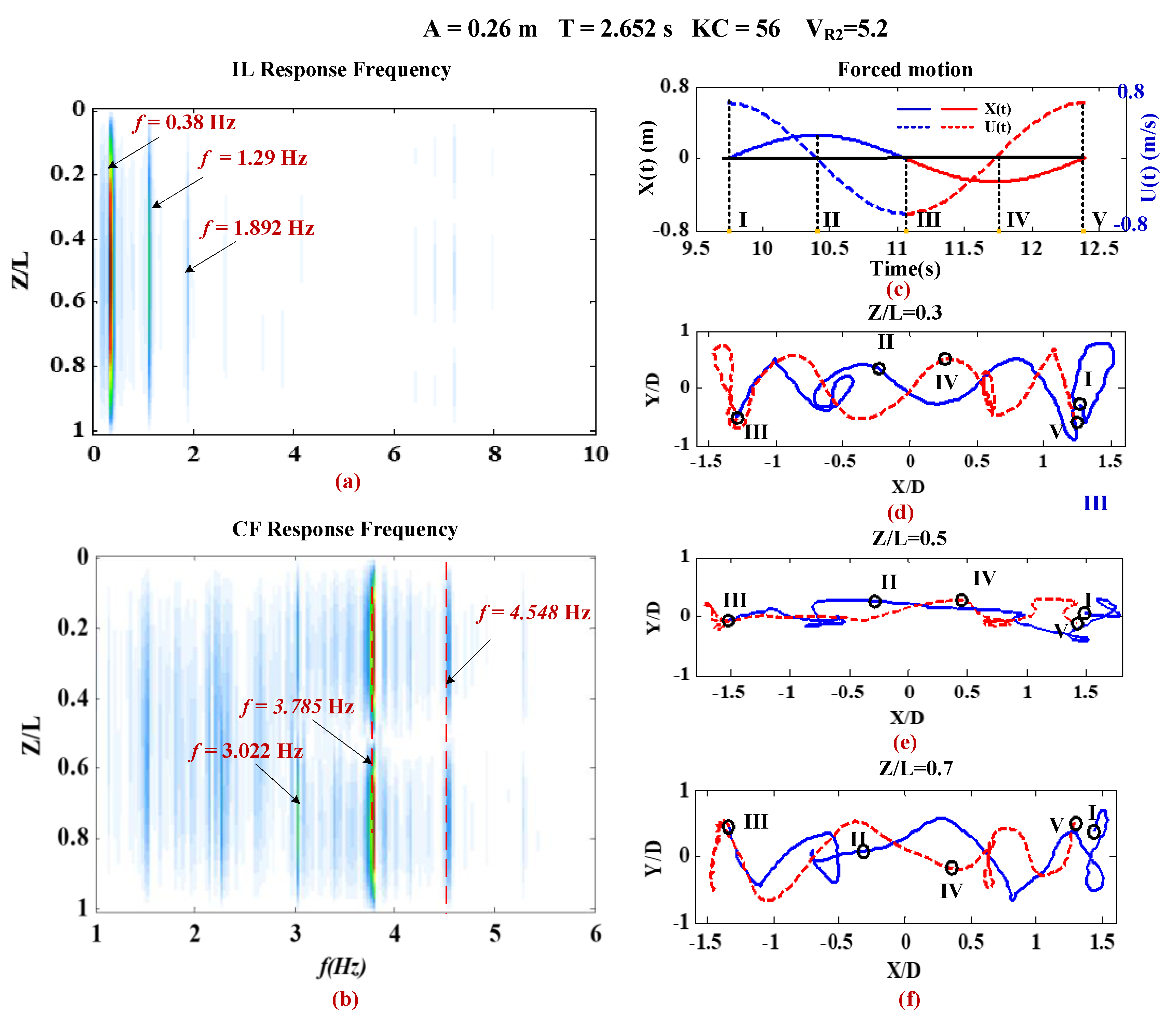
• The features of response motion trajectory under higher modes are different from those under only the first mode excited, especially for larger KC numbers. The walking “8” and “o” shapes of the motion trajectory are observed under only the first mode excited and disappear under the higher mode. The discrepancies of trajectory along the flexible pipe and in different time phases indicate that the hydrodynamic coefficient may exhibit spatial and temporal features.
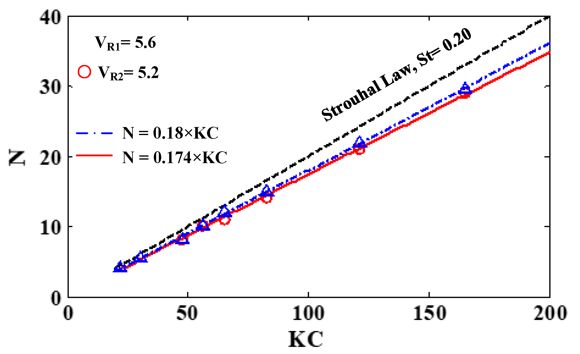
• The dominant frequency of the VIV is always kept triple that of the oscillatory flow frequency in the IL direction and maintains the Strouhal law in the CF direction. Under a V_R of approximately 5.5, the St number is equal to 0.18 and is not affected by the excited mode number.

Generally speaking, these findings will improve the basic understanding of VMI-VIV phenomena and provide a good reference for developing a VIV prediction method of a flexible pipe in an oscillatory flow.

References

1. Blevins, R.D.; Saunders, H. Flow-Induced Vibration; Elsevier: Amsterdam, The Netherlands, 1977. [Google Scholar]
2. Schewe, G. On the force fluctuations acting on a circular cylinder in crossflow from subcritical up to transcritical Reynolds numbers. J. Fluid Mech. 1983, 133, 265–285. [Google Scholar] [CrossRef]
3. Williamson, C.H.K. Defining a universal and continuous Strouhal–Reynolds number relationship for the laminar vortex shedding of a circular cylinder. Phys. Fluids 1988, 31, 2742. [Google Scholar] [CrossRef]
4. Hallam, M.G. Dynamics of Marine Structures: Methods of Calculating the Dynanic Response of Fixed Structures Sub; Ciria underwater engineering group: London, UK, 1977. [Google Scholar]
5. Achenbach, E.; Heinecke, E. On vortex shedding from smooth and rough cylinders in the range of reynolds number multiplied by 103 to multiplied by 106. J. Fluid Mech. 1981, 109, 239–251. [Google Scholar] [CrossRef]
6. Williamson, C.H.K. Sinusoidal flow relative to circular cylinders. J. Fluid Mech. 2006, 155, 141–174. [Google Scholar] [CrossRef]
7. Williamson, C.H.K.; Govardhan, R. Vortex-induced vibrations. Annu. Rev. Fluid Mech. 2004, 36, 413–455. [Google Scholar] [CrossRef] [Green Version]
8. Williamson, C.H.K.; Govardhan, R. A brief review of recent results in vortex-induced vibrations. J. Wind. Eng. Ind. Aerodyn. 2008, 96, 713–735. [Google Scholar] [CrossRef]
9. Govardhan, R.; Williamson, C.H.K. Modes of vortex formation and frequency response of a freely vibrating cylinder. J. Fluid Mech. 2000, 420, 85–130. [Google Scholar] [CrossRef]
10. Sarpkaya, T. A critical review of the intrinsic nature of vortex-induced vibrations. J. Fluids Struct. 2004, 19, 389–447. [Google Scholar] [CrossRef]
11. Bearman, P.W. Vortex shedding from oscillating bluff bodies. Annu. Rev. Fluid Mech. 1984, 16, 195–222. [Google Scholar] [CrossRef]
12. Feng, C.C. The Measurement of Vortex Induced Effects in Flow past Stationary and Oscillating Circular and D-Section Cylinder. Master’s Thesis, University of Britich Columbia, Vanccuver, BC, Canada, 1963. [Google Scholar]
13. Griffin, O.M.; Ramberg, S.E. Some recent studies of vortex shedding with application to marine tubulars and risers. J. Energy Resour. Technol. 1982, 104, 2–13. [Google Scholar] [CrossRef]
14. Parkinson, G. Phenomena and modelling of flow-induced vibrations of bluff bodies. Prog. Aerosp. Sci. 1989, 26, 169–224. [Google Scholar] [CrossRef]
15. Lie, H.; Kaasen, K.E. Modal analysis of measurements from a large-scale VIV model test of a riser in linearly sheared flow. J. Fluids Struct. 2006, 22, 557–575. [Google Scholar] [CrossRef]
16. Fu, S.; Ren, T.; Li, R.; Wang, X. Experimental Investigation on VIV of the Flexible Model under Full Scale Re Number. In Proceedings of the ASME 2011 30th International Conference on Ocean, Offshore and Arctic Engineering, Rotterdam, The Netherlands, 19–24 June 2011; pp. 43–50. [Google Scholar]
17. Ren, H.; Xu, Y.; Zhang, M.; Fu, S.; Meng, Y.; Huang, C. Distribution of drag coefficients along a flexible pipe with helical strakes in uniform flow. Ocean Eng. 2019, 184, 216–226. [Google Scholar] [CrossRef]
18. Vandiver, J.K. Drag coefficients of long flexible cylinders. In Proceedings of the 15th Annual Offshore Technology Conference, Houston, TX, USA, 1–4 May 1985. [Google Scholar]
19. Chaplin, J.R.; Bearman, P.W.; Huarte, F.J.H.; Pattenden, R.J. Laboratory measurements of vortex-induced vibrations of a vertical tension riser in a stepped current. J. Fluids Struct. 2005, 21, 3–24. [Google Scholar] [CrossRef]
20. Song, L.; Fu, S.; Dai, S.; Zhang, M.; Chen, Y. Distribution of drag force coefficient along a flexible riser undergoing VIV in sheared flow. Ocean Eng. 2016, 126, 1–11. [Google Scholar] [CrossRef]
21. Song, L.; Fu, S.; Li, M.; Gao, Y.; Ma, L. Tension and drag forces of flexible risers undergoing vortex-induced vibration. China Ocean Eng. 2017, 31, 1–10. [Google Scholar] [CrossRef]
22. Frank, W.R.; Tognarelli, M.A.; Slocum, S.T.; Campbell, R.B.; Balasubramanian, S. Flow-induced vibration of a long, flexible, straked cylinder in uniform and linearly sheared currents. In Offshore Technology Conference; Offshore Technology Conference: Houston, TX, USA, 2004; p. 8. [Google Scholar]
23. Trim, A.D.; Braaten, H.; Lie, H.; Tognarelli, M.A. Experimental investigation of vortex-induced vibration of long marine risers. J. Fluids Struct. 2005, 21, 335–361. [Google Scholar] [CrossRef]
24. Vandiver, J.K.; Li, L. SHEAR7 V4.4 Program Theoretical Manual; Massachusetts Institute of Technology: Cambridge, MA, USA, 2005. [Google Scholar]
25. Triantafyllou, M.; Triantafyllou, G.; Tein, Y.D.; Ambrose, B.D. Pragmatic Riser VIV Analysis. In Proceedings of the Offshore Technology Conference (OTC), Houston, TX, USA, 3–6 May 1999. [Google Scholar]
26. SINTEF Ocean. VIVANA 4.12.2 Theory Manual; Marintek: Trondheim, Norway, 2018. [Google Scholar]
27. Wang, J.; Fu, S.; Baarholm, R.; Jie, W.; Larsen, C.M. Out-of-plane vortex-induced vibration of a steel catenary riser caused by vessel motions. Ocean Eng. 2015, 109, 389–400. [Google Scholar] [CrossRef]
28. Wang, J.; Fu, S.; Larsen, C.M.; Baarholm, R.; Wu, J.; Lie, H. Dominant parameters for vortex-induced vibration of a steel catenary riser under vessel motion. Ocean Eng. 2017, 136, 260–271. [Google Scholar] [CrossRef] [Green Version]
29. Pesce, C.P.; Franzini, G.R.; Fujarra, A.L.C.; Gonçalves, R.T.; Salles, R.; Mendes, P. Further experimental investigations on vortex self-induced vibrations (vsiv) with a small-scale catenary riser model. In Proceedings of the ASME 2017 36th International Conference on Ocean, Offshore and Arctic Engineering, Rondheim, Norway, 25–30 June 2017. [Google Scholar]
30. Wang, J.; Fu, S.; Baarholm, R.; Jie, W.; Larsen, C.M. Fatigue damage of a steel catenary riser from vortex-induced vibration caused by vessel motions. Mar. Struct. 2014, 39, 131–156. [Google Scholar] [CrossRef]
31. Le Cunff, C.; Biolley, F.; Damy, G. Experimental and numerical study of heave-induced lateral motion (HILM). In Proceedings of the ASME 2005 24th International Conference on Offshore Mechanics and Arctic Engineering, Halkidiki, Greece, 12–17 June 2005; pp. 757–765. [Google Scholar]
32. Rateiro Pereira, F.; Gonçalves, R.T.; Pesce, C.P.; Fujarra, A.L.C.; Franzini, G.R.; Mendes, P. A model scale experimental investigation on vortex-self induced vibrations (vsiv) of catenary risers. In Proceedings of the ASME 2013 32nd International Conference on Ocean, Offshore and Arctic Engineering. Volume 7: CFD and VIV, Nantes, France, 9–14 June 2013. V007T08A029. [Google Scholar]
33. Wang, J.; Fu, S.; Wang, J.; Li, H.; Ong, M.C. Experimental investigation on vortex-induced vibration of a free-hanging riser under vessel motion and uniform current. J. Offshore Mech. Arct. Eng. 2017, 139. [Google Scholar] [CrossRef]
34. Wang, J.; Xiang, S.; Fu, S.; Cao, P.; Yang, J.; He, J. Experimental investigation on the dynamic responses of a free-hanging water intake riser under vessel motion. Mar. Struct. 2016, 50, 1–19. [Google Scholar] [CrossRef] [Green Version]
35. Fu, S.; Wang, J.; Baarholm, R.; Wu, J.; Larsen, C.M. Features of vortex-induced vibration in oscillatory flow. J. Offshore Mech. Arct. Eng. 2014, 136, 011801. [Google Scholar] [CrossRef]
36. Wang, J.; Fu, S.; Baarholm, R.; Wu, J.; Larsen, C.M. Fatigue damage induced by vortex-induced vibrations in oscillatory flow. Mar. Struct. 2015, 40, 73–91. [Google Scholar] [CrossRef]
37. Sumer, B.M.; Fredsøe, J. Transverse vibrations of an elastically mounted cylinder exposed to an oscillating flow. J. Offshore Mech. Arct. Eng. 1988, 110, 387–394. [Google Scholar] [CrossRef]
38. Ren, H.; Xu, Y.; Cheng, J.; Cao, P.; Zhang, M.; Fu, S.; Zhu, Z. Vortex-induced vibration of flexible pipe fitted with helical strakes in oscillatory flow. Ocean Eng. 2019, 189, 106274. [Google Scholar] [CrossRef]
39. Liu, C.; Fu, S.; Zhang, M.; Ren, H.; Xu, Y. Hydrodynamics of a flexible cylinder under modulated vortex-induced vibrations. J. Fluids Struct. 2020, 94, 102913. [Google Scholar] [CrossRef]
40. Fu, B.; Zou, L.; Wan, D. Numerical study of vortex-induced vibrations of a flexible cylinder in an oscillatory flow. J. Fluids Struct. 2018, 77, 170–181. [Google Scholar] [CrossRef]
41. Song, L.; Fu, S.; Cao, J.; Ma, L.; Wu, J. An investigation into the hydrodynamics of a flexible riser undergoing vortex-induced vibration. J. Fluids Struct. 2016, 63, 325–350. [Google Scholar] [CrossRef]
42. Mengmeng, Z.; Shixiao, F.; Leijian, S.; Jie, W.; Halvor, L.; Hanwen, H. Hydrodynamics of flexible pipe with staggered buoyancy elements undergoing vortex-induced vibrations. J. Offshore Mech. Arct. Eng. 2018, 140, 061805. [Google Scholar]
43. Liu, C.; Fu, S.; Zhang, M.; Ren, H. Time-varying hydrodynamics of a flexible riser under multi-frequency vortex-induced vibrations. J. Fluids Struct. 2018, 80, 217–244. [Google Scholar] [CrossRef]
Figure 1. Overview and sketch of the whole experimental setup: ((a). the overview photo; (b). the schematic drawing).
Jmse 08 00408 g001
Figure 2. The Fiber Bragg Grating (FBG) strain sensor instrumentation along the flexible pipe model.
Jmse 08 00408 g002
Figure 3. Root mean square values of the displacement modal weights in the cross flow (CF) direction for different KC numbers under VR2 = 5.2.
Jmse 08 00408 g003
Figure 4. Distribution of displacement response along the flexible pipe in the CF and in-line (IL) directions for different KC numbers under VR2 = 5.2: (a) The VIV displacement response in the CF direction; (b) The VIV displacement response in the IL direction.
Jmse 08 00408 g004
Figure 5. Time history of measured and calculated strain at different gauge points in both the CF and IL directions for KC = 56 and VR2 = 5.2.
Jmse 08 00408 g005
Figure 6. Time history of measured and calculated strain at different gauge points in both the CF and IL directions for KC = 121 and VR2 = 5.2.
Jmse 08 00408 g006
Figure 7. Distributions of the measured and calculated strains in the CF and IL directions for different KC numbers.
Jmse 08 00408 g007
Figure 8. Spatial and temporal distribution of the VIV response in the case of KC = 56 for VR2 = 5.2.
Jmse 08 00408 g008
Figure 9. The spatial and temporal distribution of the VIV response in the case of KC = 121 for VR2 = 5.2.
Jmse 08 00408 g009
Figure 10. The time history of the VIV response and time–frequency distribution at Z/L = 0.5 for VR1 = 5.6 and KC = 56: (a) The forced motion velocity; (b) The VIV displacement response; (c) The time–frequency distribution of the VIV response; (d) The time-varying frequencies.
Jmse 08 00408 g010
Figure 11. The time history of the VIV response and time–frequency distribution at Z/L = 0.3 for VR2 = 5.2 and KC = 56: (a) The forced motion velocity; (b) The VIV displacement response; (c) The time–frequency distribution of the VIV response; (d) The time-varying frequencies.
Jmse 08 00408 g011
Figure 12. The time history of the VIV response and time–frequency distribution at Z/L = 0.5 for VR1 = 5.6 and KC = 121: (a) The forced motion velocity; (b) The VIV displacement response; (c) The time–frequency distribution of the VIV response; (d) The time-varying frequencies.
Jmse 08 00408 g012
Figure 13. The time history of the VIV response and time–frequency distribution at Z/L = 0.3 for VR2 = 5.2 and KC = 121: (a)The forced motion velocity; (b) The VIV displacement response; (c) The time–frequency distribution of VIV response; (d) The time-varying frequencies.
Jmse 08 00408 g013
Figure 14. The time history of the VIV response at Z/L = 0.3 and the response of the first and second modal spaces for VR2 = 5.2 and KC = 121: (a) The forced motion velocity; (b) The VIV displacement response; (c) The time history of first modal weight; (d) The time history of second modal weight.
Jmse 08 00408 g014
Figure 15. The spatial distribution of response frequency and displacement trajectories at different positions when KC = 56 and VR1 = 5.6.
Jmse 08 00408 g015
Figure 16. The spatial distribution of response frequency and displacement trajectories at different positions when KC = 56 and VR2 = 5.2.
Jmse 08 00408 g016
Figure 17. The spatial distribution of response frequency and displacement trajectories at different positions when KC = 121 and VR1 = 5.6.
Jmse 08 00408 g017
Figure 18. The spatial distribution of response frequency and displacement trajectories at different positions when KC = 121 and VR2 = 5.2.
Jmse 08 00408 g018
Figure 19. The maximum root mean square VIV displacement responses versus KC numbers under different dominated modes.
Jmse 08 00408 g019
Figure 20. The summarized relationship between vortex-shedding pairs and KC numbers under different dominant modes.
Jmse 08 00408 g020