
Abstract
Beryllium is being adopted for plasma facing walls in fusion reactors. This has led to the observation of emissions from the A 2Π state of beryllium hydride. Use of these emissions to monitor Be erosion requires electron impact excitation rates. Cross sections for electron impact vibrational excitation within the X 2Σ+ state and vibrationally resolved electronic excitation to the A 2Π state are reported for BeH, BeD and BeT. Electron collisions are studied at a range of internuclear separations using the UK molecular R-matrix (UKRmol+) codes. Electronic excitation is studied both within the Franck–Condon approximation and by explicit averaging of the T-matrix elements. It is found that (a) inclusion of the effect of higher partial waves using the Born approximation leads to significant increases in the cross sections and (b) the Franck–Condon approximation underestimates the importance of collisions for which the vibrational state changes during electronic excitation.
Export citation and abstract BibTeX RIS

Original content from this work may be used under the terms of the Creative Commons Attribution 4.0 licence. Any further distribution of this work must maintain attribution to the author(s) and the title of the work, journal citation and DOI.
1. Introduction
The current proposal for the ITER fusion reactor is that various plasma facing walls will be made of beryllium (Kupriyanov et al 2015). In anticipation of this, the Joint European Torus (JET) (Gibson 1979, Schumacher 1983) is already testing an internal reactor wall called the ITER-like wall (ILW) parts of which are made of Be (Brezinsek et al 2015). Under these circumstances it is important to monitor the erosion of Be from the walls and emission spectra of beryllium hydride in various isotopic forms have already been observed in fusion plasma experiments (Darby-Lewis et al 2018, Duxbury et al 1998). Linking Be erosion with these emission spectra requires a theoretical understanding of the processes involved.
To model and understand emissions from BeH (BeD, BeT) requires a variety of data. First the molecule is excited in the plasma to its A 2Π state, presumably by electron collisions. Second the molecule emits from levels of the A 2Π state to ones in the ground X 2Σ+ state. Both these processes need to be fully understood. In a paper henceforth referred to as I, Darby-Lewis et al (2017) computed electron impact excitation cross sections for beryllium hydride at a single geometry corresponding to the BeH equilibrium internuclear separation. These calculations used the R-matrix method (Tennyson 2010) and were the first published which used the new UKRmol+ code (Mašín et al 2020). In general the results obtained were comparable to those obtained previously by Celiberto et al (2013) who also used the R-matrix method but in the earlier UKRmol implementation (Carr et al 2012). However, there were two important differences between the calculations; Celiberto et al (2013) used Franck–Condon (FC) factors to simulate vibrational effects in the electronic excitation process and Darby-Lewis et al (2017) used a Born correction for their dipole-allowed electronic excitation cross sections. This correction is significant for the key X 2Σ+–A 2Π excitation.
In a recent paper, designated II below, Darby-Lewis et al (2018) developed a full spectroscopic model for BeH, BeD and BeT. This model explicitly included Born–Oppenheimer breakdown (BOB) terms to isotopologue-dependent potential energy curves for the three species. This model provided an excellent fit to observed plasma emission spectra for both BeH and BeD, giving effective rotational and vibrational temperatures in the 3000–5000 K range.
To complete the inputs for a BeH/BeD/BeT radiative collisional model it is necessary to fully consider the electron impact vibrational excitation processes in the three isotopologues. This is the purpose of the current paper. Within the adiabatic nuclei approximation there are a number of ways of performing vibrationally-resolved electron impact excitation calculations. The simplest procedure, already mentioned above, involves scaling a single fixed nuclei calculation with FC factors. However, besides any non-FC effects ignored by this procedure, the FC method cannot give information on electron impact vibrational excitation within a single electronic state. Vibrational excitation cross sections or rates are needed for the radiative collisional model. In this work we therefore develop a method based on the use of vibrational wavefunctions to vibrationally average over a grid of fixed nuclei T-matrices. This procedure is significantly more computationally expensive as it requires the electron collision calculations to be performed at a grid of geometries. However, in return one recovers both any non-FC effects in the electronic excitation process and electron impact vibrational excitation cross sections. Our electronic excitation results are compared with ones computed using the FC approximation. We note that neither of these methods deals correctly with resonances formed by temporary capture of the electron in a quasibound anion state; there are special procedures available for treating resonance-driven vibrationally resolved processes (Laporta et al 2012, Laporta et al 2015). However, as discussed below, BeH has some rather narrow resonances in the electronic excitation region, see I. These resonances may provide a route to dissociative electron attachment but, due to their narrowness which means they only interact with electrons in a rather narrow energy range, are unlikely to make a major contribution to the rate of electron impact vibrational or vibronic excitation.
Vibrationally resolved cross-sections have been obtained previously using R-matrix calculations (Danby and Tennyson 1991, Rabadán et al 1998, Stibbe and Tennyson 1997, Teillet-Billy et al 1999). Indeed there have been recent calculations on both BeH (Celiberto et al 2013), discussed above, and the BeH+ cation (Laporta et al 2017, Niyonzima et al 2018). However, as part of the present study, a new vibrationally averaging program was developed. This program and how the data generated are discussed in the following section. Section 3 presents our results and a comparison between full adiabatic nuclei calculations and ones using FCs. Conclusions and ideas for future work are given in section 4.
2. Theory
Use of the adiabatic nuclei approximation can be thought of as vibrationally averaging the geometry-dependent scattering results. Here this is done by averaging over T-matrix elements, a method that has been used previously for ground state vibrational excitation calculations in the UKRmol codes (Rabadán and Tennyson 1999). Here we consider vibronic (de)excitation from any vibronic state to any other. Figure 1 gives a schematic representation of our procedure.
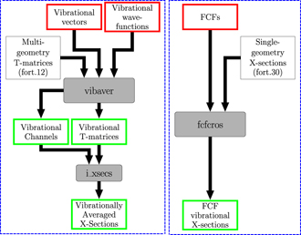
Figure 1. Flow diagram showing the two paths taken to vibrational resolution. Program modules vibaver, i_xsecs and fcfcros are shown in rounded boxes with grey backgrounds and data files are in sharp cornered boxes with white backgrounds. Output data files in green are scattering quantities, and in red are files from nuclear motion code Duo (Yurchenko et al 2016). The left blue dashed box shows vibrational resolution by the vibrational averaging of multi-geometry T-matrices, the right dashed box shows the use of Franck–Condon factors and single geometry scattering calculations. The fortran file names, fort.12 and fort.30, correspond to the defaults used by the UKRmol(+) outer region code (Carr et al 2012).
Download figure:
Standard image High-resolution imageThe fixed geometry R-matrix calculations provide a set of internuclear distance, R, and scattering energy, E, dependent T-matrix elements, Ti'',i'(E, R), where i'' and i' are channel labels. One can then compute vibrationally resolved T-matrix elements, Ti'',v'',i',v'(E), using the expression

where |ϕe'',v''(R)⟩ and |ϕe',v'(R)⟩ are vibronic wavefunctions associated with vibrational state v in electronic state e. The following two subsections give details of how the vibronic wavefunctions and fixed-nuclei T-matrices were computed.
With this procedure it is necessary to make assumptions about the total scattering energy when linking results from different geometries. This is an issue because the definition of the total scattering energy used in the scattering calculation is not geometry independent as it depends on the initial target state energy. The usual definition of the scattering energy is given as

where the total energy E is the scattering energy at which calculations are performed, El and Eu are the energies of the upper and lower states, and Ek,u and Ek,l are the electron kinetic energy linked with these upper and lower states. However, in multi-geometry calculations El and Eu vary with geometry, and thus the definition of the total scattering energy, E, also varies with geometry if, as implied by equation (1), the electron kinetic energy is taken to be geometry-independent when performing the vibrational averaging. Here we assume that Ek,l and Ek,u are geometry independent. The result of this assumption is given by the rearrangement of equation (2)

where the quantity ΔEul represents the difference in the initial and final kinetic energies which in a vibrationally averaging calculation comes to represent the difference in energy between the upper and lower vibrational states. In our model, ΔEul is the definitively geometry independent quantity. For the resultant equality assumed in equation (3) to be true the geometry dependence of the upper and lower states must cancel each other out, i.e. the potential energy curve (PEC)s must be parallel. Provided this assumption is approximately true, the concatenation of the multi-geometry results along with a constant scattering energy is valid. This is equivalent to the assumption made by Trevisan and Tennyson (2002) who studied electron impact dissociation of H2. They commented that the bond-length dependent energy Eout +  (R) is not precisely the incoming electron energy Ein, but that equating them is necessary to give a well-defined energy for the continuum function of the nuclei. In practice the curves used here are almost parallel, as can be see from the almost diagonal Franck–Condon factors computed below.
Even simpler for achieving vibronic resolution from electronic scattering results is to use the weighted averaging approach implied by the Franck–Condon (FC) approximation, where the electronic inelastic results are split into an initial vibrational state in the initial electronic level and final vibrational state in the final electronic level. The value of the weights is given by the overlap of the initial and final vibrational wavefunctions,
Of course, within a given electronic state all FC factors are zero except those between the same vibrational state meaning that the approximation only allows for vibrationally elastic collisions within a given electronic state. The FC factors can be applied directly to the fixed-geometry cross sections,

where σe'',e' is the vibronically resolved cross section obtained from the cross sections computed at a single geometry, R = Rf, and here Rf was taken as the equilibrium internuclear separation of Re = 1.3426 Å. The FC approximation makes the same assumptions about energy dependence with nuclear motion as full averaging. This method requires only a single R-matrix calculation and was used in the previous R-matrix study on BeH by Celiberto et al (2013).
2.1. Electron scattering calculations
The R-matrix method calculations were performed with the new UKRmol+ code (Mašín et al 2020) using MOLPRO (Werner et al 2012) to generate target orbitals. The calculations presented in I were repeated on a grid of geometries. These calculations used a frozen core—full configuration interaction model where the Be(1s) electrons were frozen and the other two electrons are allowed to occupy all orbitals given by the aug-cc-pVTZ basis set. A mixed Gaussian/B-spline basis set was used to represent the electronic continuum with partial waves ℓ ⩽ 6 and an R-matrix box of 35 a0. A total of 21 electronic states were considered in the outer region but only the lowest two electronic states (X Σ+ and A 2Π) concern us here. This model was extensively tested in I where further details of the calculation can be found.
We note that BeH has a permanent dipole moment and that the electronic transtion considererd here is dipole allowed. Truncation of the partial wave expansion (at ℓ = 6) does not allow for a full treatment of the long-range dipole. In I we used a Born correction (or top-up) applied directly to the cross sections as proposed by Norcross and Padial (1982) and discussed in the context of the UKRmol codes by Kaur et al (2008). For the FC calculations we simply used these Born-corrected cross sections. However, the vibrational averaging procedure produces non-Born-corrected T-matrices; in this case we separately corrected the cross sections using the appropriate Born correction for each vibrational transition.
For elastic and excitation cross sections the Born correction was applied directly to the cross sections. However, de-excitation cross sections, sometimes described as super-elastic cross sections, were computed using the principle of detailed balance:

where σl→u and σu→l are cross-sections from lower to upper and upper to lower states respectively, gl, gu are statistical weights for the lower and upper states, Ek,l Ek,u are electron kinetic energies which are related to the total energy as given in equation (2). This assumption ensures that our cross section set is self-constent.
2.2. Nuclear motion calculations
We consider two electronic states namely the X 2Σ+ ground state and the first excited state, A 2Π, with the corresponding potential energy curves (PECs) represented analytically using a Morse long-range (MLR) potential (Le Roy and Henderson 2007) and an extended Morse oscillator (EMO) potential (Lee et al 1999), respectively. In addition the model included curves which represent spin–orbit (LS) coupling both within the A 2Π state and between the X to A states. Calculations were performed using Hund's case (a); see Tennyson et al (2016a) for a review of this approach. All curves were taken from II where (a) they were tuned to the available observed spectroscopic data for BeH, BeD and BeT due to Shayesteh et al (2003) and Le Roy et al (2006), and (b) explicit allowance was made for Born–Oppenheimer breakdown (BOB), using the formulation of Le Roy (2017), in the fit leading to slightly different curves for each isotopologue. The resulting spectroscopic model was used to give comprehensive rovibronic line lists for the three isotopologues which can be obtained from the ExoMol data base (Tennyson et al 2016b).
In order to produce a full vibrationally resolved model of the R-matrix data we need these data for a range of geometries. So the single geometry calculation from I above is repeated, varying the internuclear separation in the calculation, which is done on the input to MOLPRO. The target and scattering models selected in the single geometry case are used in all the multi geometry calculations. The validity of the target model was checked prior to its confirmation in the single geometry case. Evidence for this is shown in the comparison of the PECs from the chosen target model to those from the literature (Pitarch-Ruiz et al 2008) and the fitted PECs from II, see figure 2.
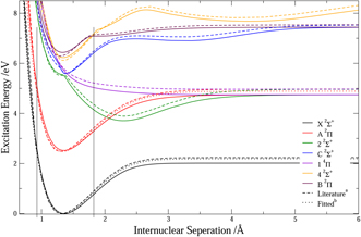
Figure 2. PEC comparison of the aug-ccpVDZ FC–FCI target model (solid lines) with those of Pitarch-Ruiz et al (2008) (dashed lines), and the fitted PECs from II (Darby-Lewis et al 2018) (dotted lines). The zero energy is taken as the minimum of the X 2Σ+ ground state for each calculation. The vertical black lines show the region in which the multi-geometry electron scattering calculations were used in the vibrational averaging model.
Download figure:
Standard image High-resolution imageVibronic wavefunctions were generated using the curves described above and the variational nuclear motion program Duo (Yurchenko et al 2016). Here only the lowest angular momentum states (in this case  ) were considered for each electronic state. Duo was also used to generate FC factors from the vibronic wavefunctions.
While the BOB-corrected curves for BeH, BeD and BeT are very similar, there are significant differences in the level spacing and the corresponding vibronic wavefunctions between the three isotopologues. This is due to mass effects which lead to closer energy spacing and reduced zero point energies as BeH becomes BeT.
3. Fixed geometry results
UKRmol+ calculations were performed at about 100 points in the range R = 0.1–9.0 Å. Even allowing for use of MPI (message passing interface) for key parts of the calculation (Al-Refaie and Tennyson 2017), these runs took 30 000 h of CPU time to complete on UCL's Legion/Myriad/Grace computer clusters. The multi geometry results show smoothly varying cross-sections with geometry, see figure 3. For the present studies, however, only the 11 geometries lying in the range 1.0 ⩽ R ⩽ 1.9 Å were actually used in the vibrationally averaging procedure. This restricted range covers the FC region and avoids complications with curve crossings which occur at both short and longer internuclear separations. These curve crossings occur at higher energies and at geometries where the overlap with the low-lying ground state vibrational states is negligible so their exclusion should not materially affect the results.

Figure 3. X–A cross sections, σ, as a function of the internuclear separation, R, and scattering energy, E. The main resonance can be seen moving to lower energy with increasing internuclear separation.
Download figure:
Standard image High-resolution imageFigure 3 displays the ground state (GS), X 2Σ+, to the first excited state, A 2Π, electronic excitation cross section as a function of geometry and scattering energy. This figure shows that the position of resonance feature(s), seen as spike(s), moves to a higher energy as the internuclear separation decreases. They proved quite difficult to fit with the standard Breit–Wigner form (Tennyson and Noble 1984) but table 1 gives the position of the main feature as a function of geometry. The non-smooth behaviour of the resonance feature can complicate the vibrational averaging calculations but, as their averaged contribution to the vibrationally-resolved cross sections is small, we chose to simply ignore it. We note that pseudo-resonanaces are a feature of calculations performed at higher scattering energies such as the ones above the energies of the highest target energies included in the model. In our present study, these occur at energies which are probably too high to matter for ITER but their effect can be seen in some figures below.
Table 1. The 3Π resonance position as a function of geometry, this resonance being visible in the X–A cross-section in figure 3. For the equilibrium geometry, marked witha, the resonance position was fitted, at other geometries the position is estimated.
| R (Å) | Position (eV) |
|---|---|
| 1.0 | 6.55 |
| 1.1 | 6.3 |
| 1.2 | 5.95 |
| 1.3 | 5.6 |
| 1.3426 | 5.487a |
| 1.4 | 5.2 |
| 1.5 | 4.75 |
| 1.6 | 4.3 |
| 1.7 | 3.9 |
| 1.8 | 3.45 |
| 1.9 | 3.05 |
The R-matrix scattering calculation was carried out up to a total scattering energy of 7.5 eV. This energy represents the initial electron kinetic energy of the impacting electron and the corresponding total energy of the system is dependent on the geometry-dependent energy of the target molecule. Due to the highly parallel nature of these two PECs, see figure 2, the vertical excitation energy is almost constant at ≈2.5 eV over the region of interest. This means that the threshold, the starting scattering energy for the electronic excitation cross-section, is almost constant at this value.
For the calculation of rates, the energy range of the cross-section was extended by extrapolation using a total Born cross-section. The extrapolated portion of the cross-section is scaled to the magnitude of the R-matrix + Born top-up cross-section at 7.5 eV to ensure continuity. The extrapolated cross sections allow for the high energy tail of the Maxwell–Boltzmann to be accounted for. Vibrationally-resolved calculations considered states v ⩽ 9, although for clarity the figures below usually show excitation starting from v = 0 and excitation to only a few upper vibrational states. In the various cross-section figures in this section BeH, BeD, and BeT are represented in solid, dashed and dotted lines respectively.
4. Vibrational excitation
Total vibrational excitation cross sections can only be computed using the vibrationally-averaged multi-geometry T-matrices calculated above. Figure 4 shows cross-sections for the transitions from the initial v = 0 vibrational ground to states with v = 1–3 within the X 2Σ+ ground electronic state. Within the Franck–Condon model these cross sections are all elastic, i.e. Δv = 0. It can be seen that the vibrational excitation cross sections are not small with excitation to all states with v = 1–3 showing large cross sections near their threshold for vibrational excitation and Δv = 1 cross sections remaining large at all energies. The structures, which become increasingly apparent with increasing electron impact energies, are probably artifacts of our calculation method. These are averaged over in the construction of rates which is probably the correct approach to dealing with them.
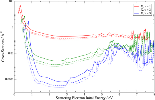
Figure 4. Vibrational excitation cross-sections within the X 2Σ+ ground electronic state for the full vibrational averaging, multi-geometry model from the v = 0 to states v = 1 → 3. With BeH in solid, BeD in dashed, and BeT in dotted lines as shown in the legend.
Download figure:
Standard image High-resolution image4.1. Vibrationally-resolved electronic excitation
Figure 5 shows our results for the vibrationally-resolved X 2Σ+ to A 2Π electronic excitations computed using our vibrationally resolved T-matrices. It can be seen that the electronic excitation process is dominated by the Δv = 0 excitation step which is the expected result arising from the near parallel X and A state curves. However, transitions with Δv > 0 are not negligible. These transitions show significant structure due to resonances and probably also some numerical artifacts in our calculations. These should generally be disregarded; they have little influence on the rates.
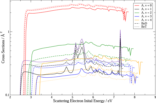
Figure 5. Vibronic cross-sections for the full vibrational averaging, multi-geometry model for the initial state X 2Σ+, v = 0 and final state A 2Π, v = 0 → 4 with BeH (solid lines), BeD (dashed lines), and BeT (dotted lines) as shown in the legend.
Download figure:
Standard image High-resolution imageFigure 6 compares our vibrationally-resolved electronic excitation cross sections computed with full vibrational averaging with those obtained using the Franck–Condon approximation. There are marked differences between the vibrational averaging and the FC methods in the off-diagonal transitions (v = 0 to v > 0). It would appear that the FC approximation significantly underestimates the possibility of changes in vibrational quantum number on electronic excitation in this case. We also note that FC results appear to show greater variation between the isotopologues. However this is mostly due to the Born correction being applied and the fact that it makes a more significant relative contribution to the smaller cross-sections. This is because while the FC cross sections are generally smaller than for the vibrationally-averaging model, the Born top-up being applied is almost the same in both models as it depends mostly on the dipoles from the Duo calculation.

Figure 6. Born corrected vibronic cross-sections comparison with initial state X 2Σ+, v = 0 and final states A 2Π, v = 1 → 3 for BeH/D/T as shown in the legend. Since the explicitly vibrationally averaged (vibaver) cross sections are uniformly larger than the quasi-FCF ones a black dividing line has been placed in the figure to guide the eye. The vibrational averaging model cross-sections are those which lie above the black dividing line at higher energies, while those below it the higher energies are the results of the quasi-FCF calculation.
Download figure:
Standard image High-resolution imageThis similarity between the single-geometry FC and multi-geometry vibrationally averaged cross sections after application of the Born correction is shown most strongly in the vibronically elastic (Δv = 0) components where there are large dipoles. This makes the Born correction in these cases more significant to the cross-sections than the R-matrix results themselves. Vibronically elastic Born corrected results for BeH using the full multi-geometry model (there is insignificant difference in these elastic components for the single-geometry model) are shown in figure 7. The equivalent results for BeT are given in figure 8 to show the two extremes of the elastic cross-sections, with the BeD results falling predictably in between these two sets. The first thing to point out in these results is that the cross-section of the elastic X 2Σ+ vibrational state curves increases with increasing vibrational quanta, the scattering being more likely for the higher vibrational states. In contrast, in the A 2Π vibrational states this situation is reversed and the scattering is more likely for lower vibrational quanta. A second point is the difference between BeT and BeH, where though the X states intensities do not change significantly the BeH A state cross-sections show a larger increase for higher vibrational quanta. As these cross-sections are dominated by the Born correction, these effects are mostly the result of the vibrational dipoles from the Duo calculations. The cross-sections here are orders of magnitude greater than in the equilibrium geometry case due to the fact that the vibrational dipoles are much greater than the equilibrium geometry dipoles. This results from the electronic transition dipole crossing through zero close to the equilibrium point and this effect also leads to the Δv = 1 cross-sections being greater than the cross-sections Δv = 0 as has been seen above. This a consequence of the fact that the electronic transition dipole crosses through zero close to equilibrium making the equilibrium dipole small compared to the vibrationally averaged dipole.

Figure 7. Elastic cross-section BeH states X 2Σ+, v = 0 → 9 (lower set of curves) and states A 2Π, v = 0 → 9 (upper set of curves).
Download figure:
Standard image High-resolution image
Figure 8. Elastic cross-section BeT states X 2Σ+, v = 0 → 9 (lower set of curves) and states A 2Π, v = 0 → 9 (upper set of curves).
Download figure:
Standard image High-resolution image
Comparing our results with those of Celiberto et al (2013) there are two significant differences. First their rates are functional forms fitted to the magnitude of the R-matrix cross-sections and as such they suffer from the neglect of the Born corrections. Second their use of FC factors leads to the cross sections with Δv ≠ 0 being underestimated.
5. Conclusions
We have produced vibrationally resolved electron impact cross sections for both electronically elastic and inelastic processes in BeH, BeD and BeT. Our cross sections are significantly larger (approximately twice) those published previously. The Franck–Condon approximation cannot provide pure vibrational excitation cross sections but we also find that it underestimates the vibrational changes upon electronic excitation. These cross sections, alongside the spectroscopic model constructed previously (Darby-Lewis et al 2018), provide the necessary input for constructing a complete beryllium hydride collisional-radiative model. The data computed in this paper is available from the International Atomic Energy Authority (IAEA) atomic and molecular database Aladdin at https://amdis.iaea.org/ALADDIN/.
Acknowledgments
We thank the Engineering and Physical Sciences Research Council (EPSRC) for studentship (EP/M507970/1) and the Culham Centre for Fusion Energy (CCFE) for funding. The author acknowledgment the use of the UCL Legion, Myriad and Grace High Throughput/Performance Computing Facilities and associated support services in completion of this work.