


1 Introduction
The loss of ice from Antarctica is one of the main contributors to global sea-level rise (Church and White, Reference Church and White2011). It has recently started to accelerate (Nerem and others, Reference Nerem2018; Shepherd and others, Reference Shepherd2018), and is projected to increase in the next century (Ritz and others, Reference Ritz2015; DeConto and Pollard, Reference DeConto and Pollard2016). The observed increased mass loss is predominantly a response to intensified submarine melting and an increase in the rate of iceberg calving from the ice shelves (Rignot and others, Reference Rignot, Jacobs, Mouginot and Scheuchl2013; Shepherd and others, Reference Shepherd2018). On a continent-wide scale, these two processes are estimated to account for approximately the same amount of mass loss, with the relative influence of each process varying across different ice-shelf systems (Rignot and others, Reference Rignot, Jacobs, Mouginot and Scheuchl2013). Both processes have far-reaching effects, since the associated release of cold and fresh meltwater affects the water column and sea-ice formation (e.g. Hellmer, Reference Hellmer2004), both near the ice sheets and farther afield due to offshore transport by icebergs (Bigg, Reference Bigg2015). Depending on where they occur, both basal melting and iceberg calving could have implications for the stability of large parts of the ice sheet (e.g. Fürst and others, Reference Fürst2016; Reese and others, Reference Reese, Gudmundsson, Levermann and Winkelmann2018).
Since calving is an important mass-loss process for ice sheets and is currently not well constrained in ice-sheet models, it has received significant recent attention; a number of studies have aimed to establish empirical or semi-empirical calving laws to predict future calving events. Large-scale calving is the final step of a longer, cyclical process that typically begins with the formation of a crevasse at the surface or base of an ice shelf (e.g. van der Veen, Reference van der Veen1998; Fricker and others, Reference Fricker, Young, Allison and Coleman2002). Crevasse formation is mainly a function of the state of stress in the ice and occurs when the stresses surpass the yield stress of the ice (e.g. Alley and others, Reference Alley2008; Benn and Åström, Reference Benn and Åström2018). The crevasse can eventually extend over the whole ice thickness and, after horizontal propagation or intersection with another rift close to the ice front, will lead to the calving of an iceberg, the size of which depends on the rift locations. There are three main approaches to parameterize calving laws: (i) relate an assumed yield stress of ice to simulated longitudinal stresses (e.g. Morlighem and others, Reference Morlighem2016); (ii) consider crack initiation and propagation more explicitly (e.g. Benn and others, Reference Benn, Hulton and Mottram2007; Åström and others, Reference Åström2013; Bassis and Jacobs, Reference Bassis and Jacobs2013; Benn and others, Reference Benn2017); and (iii) use insights from continuum damage mechanics or fracture mechanics to formulate calving relations (e.g. Pralong and others, Reference Pralong, Funk and Lüthi2003; Borstad and others, Reference Borstad2012; Krug and others, Reference Krug, Weiss, Gagliardini and Durand2014, Reference Krug, Durand, Gagliardini and Weiss2015). See Benn and Åström (Reference Benn and Åström2018) for a recent review of glacier and ice-shelf calving.
Ice-sheet models to date have focused on the viscous deformation of ice, typically accounting for the creep of ice by applying a version of Glen's flow law (Glen, Reference Glen1955). The relative impact of elastic and viscous stress–strain relations on calving have not been studied in detail. However, previous studies have suggested that glacial ice can deform elastically in some cases, particularly on shorter timescales, such as the hourly to sub-daily timescales associated with tidal forcing (e.g. Vaughan, Reference Vaughan1995; Sayag and Worster, Reference Sayag and Worster2011, Reference Sayag and Worster2013). More recently, Wagner and others (Reference Wagner2014, Reference Wagner, James, Murray and Vella2016) suggested that the elastic theory could explain deformations in response to suddenly applied hydrostatic bending forces that usually occur over a short period of time before a major calving event, when the collapse of the ice cliff above the waterline leads to sudden perturbations of the hydrostatic equilibrium at the ice front. In addition, James and others (Reference James, Murray, Selmes, Scharrer and O'Leary2014) showed that the deformation and calving cycle of Helheim Glacier in Greenland during summer occurs over periods of a few weeks. Trevers and others (Reference Trevers, Payne, Cornford and Moon2019) analyzed the effect of similar hydrostatic imbalances in a viscous framework. However, this timescale may be too short to reflect purely viscous creep, which broadly dominates on timescales of at least a few months (Sayag and Worster, Reference Sayag and Worster2013), suggesting that elastic effects can be important for this type of buoyancy-driven calving.
In this paper, we investigate the relative roles of elastic and viscous deformations that result from underwater ice protrusions at the ice front in the calving process (Fig. 1). Such protrusions have previously been observed at tidewater glaciers (Wagner and others, Reference Wagner, James, Murray and Vella2016, Reference Wagner2019) and icebergs in temperate waters (Scambos and others, Reference Scambos, Sergienko, Sargent, MacAyeal and Fastook2005; Wagner and others, Reference Wagner2014). In these cases, the presence of warmer water and enhanced mixing near the ocean surface leads to higher melt rates close to the waterline, which, in turn, create an overhanging ice cliff above the ocean surface. Such cliffs quickly succumb to gravitational stresses and their collapse leaves behind a growing underwater protrusion. The submerged protrusion, or "ice foot", induces buoyancy forces that trigger an upward bending of the ice front. The resulting shape of the ice surface (perpendicular to the ice edge) has been referred to as a ‘rampart-moat’ profile (Scambos and others, Reference Scambos, Sergienko, Sargent, MacAyeal and Fastook2005) and features an elevated ice front (rampart) seaward of a depression below the isostatic equilibrium height of the ice surface (moat). For a sufficiently formed rampart-moat profile, the associated tensile stresses may be sufficiently high to trigger calving, a process that has been referred to as the ‘footloose’ mechanism (Wagner and others, Reference Wagner2014).
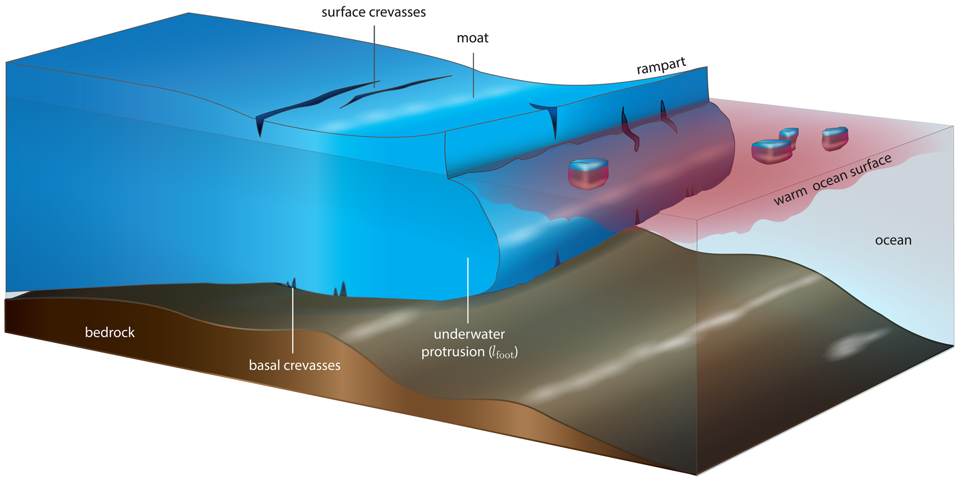
Fig. 1. Illustration of an ice shelf featuring an underwater protrusion. The protrusion is the result of increased melting at the waterline due to warm surface waters and wave erosion. The net-buoyant protrusion results in a bending force (of length lfoot) that causes the front of the ice shelf to rise up, thus forming a rampart-moat surface profile, where the ice front is higher than the hydrostatic equilibrium point (rampart) and counterbalanced by a depression below hydrostatic equilibrium (moat) farther inland (Scambos and others, Reference Scambos, Sergienko, Sargent, MacAyeal and Fastook2005). The rampart-moat profile is exaggerated for better illustration of the feature, and simulations carried out here use an idealized geometry.
Recent observations of the Ross Ice Shelf, collected with laser altimetry as part of the ROSETTA-Ice airborne surveys (2015–2017; Tinto and others, Reference Tinto2019) have detected pronounced rampart-moat profiles along a substantial fraction of the ice front (Fig. 2). While current survey techniques are not able to directly observe underwater feet at such large ice shelves, the striking profile illustrated in Figure 2 is suggestive of the presence of a submerged foot and serves as a main motivator for the present study.

Fig. 2. Laser altimetry profile collected during the ROSETTA-Ice airborne survey (2015–2017; Tinto and others, Reference Tinto2019). (a)–(b) location of the profile on Ross Ice Shelf front; (c) height above sea level along the profile for the 1500m closest to Ross Ice Shelf front, which exhibits a rampart-moat surface profile. Raw data (blue dots) have been corrected for tides and mean dynamic topography and referenced to the EIGEN-6C4 geoid. Black line is a smoothed version of the profile constructed using a Gaussian filter.
The footloose mechanism has emerged as a plausible explanation for the occurrence of the rampart-moat profile; however, it is not well understood whether the deformations associated with the footloose mechanism are predominantly elastic or viscous. Here, we briefly review the mechanical theory supporting each framework, and discuss both the viscous and elastic frameworks and their finite element numerical implementation (Section 2). We investigate the impact of the size of an underwater protrusion on the state of stress and strain for both theories (Section 3) and discuss the effects of parameters specific to each theory (Section 4).
2 Methods
2.1 Frameworks and models
A complete constitutive relation for ice should encompass elastic deformation, creep or viscous deformation, plastic deformation and fracturing. Following the initiation of a stress, isotropic polycrystalline ice first experiences an elastic deformation where the internal strain increases linearly with stress. This stage is followed by different phases of creep where the stress depends on the strain rate rather than the strain itself. Eventually, the ice reaches plasticity or brittle deformation where the stress surpasses the yield stress of ice (Cuffey and Paterson, Reference Cuffey and Paterson2010). In this paper, we focus on describing and comparing the elastic and viscous deformations that usually occur prior to plastic deformation or fracturing.
The numerical approach used to solve the viscous creep of ice is available in the Elmer finite element software developed at the Center for Science in Finland (CSC-IT; http://www.csc.fi/elmer/) and its glaciological extension Elmer/Ice. Elmer/Ice is an open-source, thermo-mechanically coupled 3-D ice-flow model (Gagliardini and others, Reference Gagliardini2013). The code is based on a 3-D numerical integration of the Stokes equations (Appendix 1).
A linear elastic framework (Appendix A.2.1) is also available in Elmer but is not fully integrated with the Elmer/Ice branch. Here, we therefore modeled the elastic response of the ice shelf to ocean forcing by adapting the classical deformation of 2-D linear elastic bodies. We validate this model by comparing it to the 1-D elastic beam theory of Wagner and others (Reference Wagner2014) and then contrast the elastic results with those of the viscous framework (the 1-D elastic beam theory is summarized in Appendix A.2.2). We note that a comprehensive treatment of this subject will eventually require a fully viscoelastic constitutive relation (e.g. Christmann and others, Reference Christmann, Müller and Humbert2019). However, we believe that significant physical insight can be gained from considering the viscous and elastic end-member scenarios as done here.
2.2 Numerical setup
Elmer/Ice was designed and written to simulate realistic 3-D geometries for ice-sheet modeling. However, due to the high resolution required to correctly represent the ice-front geometry (~2 m at the front), and to allow for intuitive insight into the complex underlying physical processes, we limit this study to an idealized 2-D flowline case. Our domain is the region near the ice-shelf front, extending 10 km inland (upstream) of the ice front. This distance has been tested to ensure that solutions are independent of the boundary conditions at the inland end of the ice shelf. We use a finite-element mesh containing 133 845 to 139 186 nodes (264 162 to 274 748 elements), depending on the size of the foot, composed of linear triangles at two resolutions: fine (2 m) over the first 1.5 km and on the underwater foot, and coarse (10 m) in regions far from the front. The elastic framework uses linear elements while the viscous framework uses linear elements stabilized using a residual-free-bubbles formulation (Baiocchi and others, Reference Baiocchi, Brezzi and Franca1993). The initial ice thickness (h) is constant at h = 200 m, while the idealized 2-D foot geometry – before deformation – consists of a rectangle of varying length (l foot) with a top surface located 10 m below sea level (Fig. 1). Densities are set to ρi = 850 kg m−3 for the ice shelf (Keys and others, Reference Keys, Jacobs and Barnett1990), assuming a constant density over the entire ice column, and ρw = 1028 kg m−3 for water. We note that the column-averaged ice density is slightly lower than that of pure ice, to roughly account for the presence of a surface firn layer. We also tested the impact of an increase in column-averaged density by considering the case for the entire column being pure ice (ρi = 917 kg m−3). To investigate how the states of stress and strain vary in the viscous and elastic frameworks, we apply a range of different perturbations at the ice front, which correspond to varying the foot length l foot between 0 and 100 m. The scenario where l foot = 10 m represents a relatively small perturbation (similar to that observed by Wagner and others, Reference Wagner2014, for an ice island in Baffin Bay), while l foot = 100 m can be regarded as an upper-limit scenario, considering the frontal elevation it would trigger with respect to available observations (e.g. Scambos and others, Reference Scambos, Sergienko, Sargent, MacAyeal and Fastook2005). In the numerical setup, the ice shelf is initially floating with a surface height above sea level equivalent to the isostatic equilibrium point without an ice foot and is then suddenly subjected to buoyant forces from an ice foot.
In the viscous framework, the ice temperature is fixed to T = −15°C when testing the effect of the different foot lengths. However, strain rates are non-linearly dependent on stresses and can be affected by ice fluidity and therefore ice temperature (as shown in Eqns (A4) and (A5)). To investigate this temperature dependence, we conduct 20 simulations with temperature varying from T = −20 to 0°C and holding l foot constant (at 50 m). These simulations broadly cover the range of observed temperatures for ice shelves (Holland and Jenkins, Reference Holland and Jenkins1999) and act as a testbed for the sensitivity of stresses and deflections of the ice to changes in temperature. In the elastic framework, by contrast, the linear stress–strain relation depends on the Young's modulus E and the Poisson's ratio ν of ice. We conduct simulations with both a 1-D elastic beam and a 2-D ice-shelf model, using a standard Poisson's ratio for ice of ν = 0.3. In addition, we test two different Young's moduli: E = 1 GPa and E = 10 MPa. While the first falls in the range of standard Young's modulus values used for pure ice (1–10 GPa), the second value is significantly lower and invoked to account for flaws in the ice that lower its bending stiffness. This suppression of the Young's modulus is discussed further in Section 4.3.
3 Results
For each foot length, l foot, we run simulations to equilibrium and compare the maximum frontal elevation, the distance from the front to the location of maximum stress and, in the viscous case, the time required to approach the maximum frontal elevation (Table 1).
Table 1. Summary of the results obtained with different l foot for the viscous model, the elastic numerical 2-D model and the elastic analytical 1-D model

The three rows correspond to (from top to bottom): The time (in years) required to reach the maximum frontal elevation (in the viscous case), the maximum frontal elevation (in meters), and the distance from the front to the location of maximum stress at the ice base (x*, in meters). For short feet, the maximum stress can be located at the ice surface (rather than its base) and its position is indicated with a triangle (▾). Elastic responses are instantaneous; therefore, we do not report times for the elastic cases.
3.1 Viscous rheology
Following other studies (e.g. Benn and others, Reference Benn2017; Trevers and others, Reference Trevers, Payne, Cornford and Moon2019), we calculate the effective principal stress (EPS), which accounts for the effect of hydrostatic water pressure and its ability to widen crevasses. EPS is defined as

where σij are the different components of the stress tensor and p w is the water pressure. Note that, while the EPS is probably most useful to predict if a stress will trigger a calving event or not, some of our results are presented in term of deviatoric stress (τ) to facilitate the comparison between the 2-D models and the 1-D elastic beam model. Figure 3 shows the EPS distribution using the viscous framework for a case without a foot and three different values of l foot (10, 50 and 100 m) and a constant ice temperature T = −15°C. The stresses in Figure 3 are computed (i) after a short period of relaxation following the ice-foot perturbation, t = 0.001 a (~9 h, corresponding to the first time step of the simulation, Figs 3a–c) and (ii) after the complete formation of the rampart-moat profile (Figs 3d–f).

Fig. 3. Early-stage (t = 0.001 a) snapshots of the spatial distribution of EPS for the viscous case, for the first 1000 m upstream of the ice front, for various lengths of underwater foot: (a) 0 m, (b) 10 m, (c) 50 m and (d) 100 m. (e)–(h) Snapshots of the spatial distribution of EPS, once the rampart-moat is fully formed.
The presence of the foot induces an upward bending moment that triggers tensile stresses at the ice base and compressive stresses in the upper part of the shelf, with a magnitude that increases as l foot increases. The areas of compression and extension are separated by a stress-free zone typically called the neutral surface. For a short foot (e.g. l foot = 10 m), the neutral surface features additional complexity that arises from the competition between a downward bending moment due to the imbalance of ice and water pressures at the front (Reeh, Reference Reeh1968) and an upward bending moment due to the buoyancy of the foot itself. For a longer foot (i.e. l foot ≥ 25 m), the buoyancy forces largely exceed those associated with the downward bending moment and only the upward flexural signal remains visible, similar to the deformations of tabular icebergs observed by Scambos and others (Reference Scambos, Sergienko, Sargent, MacAyeal and Fastook2005).
The ice shelf deforms over time and the rampart-moat profile becomes more pronounced until it reaches hydrostatic equilibrium (Fig. 4a). The time to reach this equilibrium ranges from a few months to a few years, depending on l foot. As a general rule, the longer the foot the faster equilibrium is reached, with most of the deformation developing in the first few months in all cases. The relatively long adjustment time (8 a) for the case with no foot (l foot = 0 m) comes from the aforementioned imbalance between hydrostatic and glaciostatic pressure at the ice front, which generates a downward moment at the front that can take time to reach a new equilibrium. For comparison, Reeh (Reference Reeh1968), using viscous beam theory, reports a time ranging from 0.26 to 5.2 a for a 200 m thick ice shelf (without a foot) and for temperatures between 0 and − 12°C. The maximum frontal elevation also increases with l foot, reaching 12.6 m after 4 years for l foot = 50 m and 19.3 m after just 1 year for l foot = 100 m. The shortest ice foot, l foot = 10 m, results in a maximum elevation of ~0.75 m, which is achieved in about 0.2 a (Figs 5a–c; Table 1 for more results).

Fig. 4. Temporal evolution of various parameters for the viscous case and for three different foot lengths. (a) The maximum frontal elevation at the ice front (x = 0 m); (b) the maximum deviatoric tensile stress at the ice base $\tau ^\ast$ ; and (c) the position of the maximum tensile stress $x^\ast$
 .
.
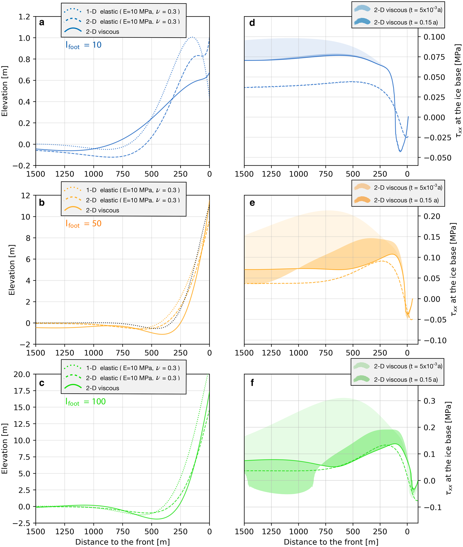
Fig. 5. Left: rampart-moat geometry predicted by viscous and elastic (E = 10 MPa and ν = 0.3) models, for various lengths of underwater foot for the 1500 m closest to the ice front: (a) l foot = 10 m; (b) l foot = 50 m; and (c) l foot = 100 m. The 1-D analytical elastic rampart-moat solution for the parameters E = 2 MPa and l foot = 40 m, discussed in Section 4.2, is plotted in black in panel (b). Right: longitudinal deviatoric stress at the ice base for the viscous and 2-D elastic frameworks, for each value of l foot. The shading represents the envelope of the stresses for the viscous framework from the beginning of the simulation (light shades) and from 0.15 a (dark shades) to the final stress (continuous lines). The 2-D elastic stresses are shown as dashed lines.
The maximum longitudinal deviatoric stress, $\tau ^\ast = \tau _{{\rm max}\comma xx}$ , relaxes over time as the rampart-moat profile forms and reaches a minimum when hydrostatic equilibrium is attained (Fig. 4b). The non-linear evolution of the stress is directly linked to the non-linear evolution of the strain rate, which can be quantified by how fast the front rises. This results in a maximum stress which drops correspondingly quickly, with the rate being highest in the first months of the viscous relaxation.
The decrease in maximum stress over time is indicative of a more general relaxation of stresses in the ice shelf and therefore at the ice base (Figs 5d–f), with the magnitude of $\tau ^\ast$ significantly reduced when t = 0.15 a (the approximate timescale at which the viscous response of ice may outweigh the elastic response of ice; Sayag and Worster, Reference Sayag and Worster2013), and further reduced when the front reaches its maximum elevation (i.e. when hydrostatic equilibrium is reached, t = 0.2 −8 a).
The decrease in stress over time is further accompanied by a shift in the location of maximum stress, $x^\ast = x\lpar \tau ^\ast \rpar$ , closer to the front of the ice shelf (Fig. 4c). At t = 0.005 a, $x^\ast = 1073$
 , 715 and 572 m, for l foot = 10, 50 and 100 m, respectively; compared to $x^\ast = 530$
 , 131 and 107 m by the time hydrostatic equilibrium is reached (Table I). Note that the distance $x^\ast$
 is also directly linked to l foot, with $x^\ast$
 decreasing as l foot increases.
A sensitivity analysis of the viscous model to the ice temperature shows a direct dependence of the time required by ice to adapt to the buoyancy forces and to reach a new hydrostatic equilibrium, monotonically decreasing as the temperature increases (Fig. 6a). Indeed, from Eqns (A2) and (A4), we find that strain rates decrease when the fluidity A (thick gray line in Fig. 6a) decreases, meaning that ice responds more slowly to external stresses when it is colder, as expected. We find that the time needed by the ice shelf to fully accommodate the stresses triggered by the hydrostatic perturbation of the foot ranges (non-linearly) from 2.5 months for T = 0°C to more than 7 years for T = −20°C. This is in agreement with previous work by Sayag and Worster (Reference Sayag and Worster2013), who estimated that the viscous bending timescale of ice sheets broadly ranges between 2–3 months and 20 years.

Fig. 6. (a) Relaxation time required to reach the maximum frontal elevation for 20 viscous simulations with ice temperature values ranging from − 20 to 0°C, for l foot = 50 m. Each blue dot represents a simulation corresponding to a temperature value on the x-axis. The thick gray curve represents the inverse of the fluidity A-1, calculated from Eqn (A5) with Q = 60 kJ mol−1 if T < −10°C and Q = 115 kJ mol−1 if T > −10°C (Cuffey and Paterson, Reference Cuffey and Paterson2010). (b) Final rampart-moat shape for the 20 simulations with temperature ranging from − 20 to 0°C (blue); analytical elastic solutions for the same foot length and Young's modulus E 1−D = 10 MPa predicting a similar front elevation (dotted blue line), and for l foot = 40 m and E 1−D = 2 MPa inferred to best fit the viscous rampart-moat shape (dotted red line). (c) Maximum Cauchy stress at the ice base for the 20 viscous simulations. In both (b) and (c), the 20 viscous rampart-moat profiles and viscous stress distributions are shown but almost perfectly coinciding.
The new hydrostatic equilibrium surface profile exhibits the same final geometry (i.e. rampart-moat shape) regardless of the temperature. That is to say the strain and stress distributions resulting from the new hydrostatic equilibrium are independent of ice fluidity (Figs 6b–c). This contrasts with the strain-rate dependence discussed above.
3.2 Elastic rheology
The elastic simulations were initialized with the same geometries as in the viscous case. Simulations with both a 1-D elastic beam and a 2-D ice-shelf model were conducted. For both models, using a standard elastic modulus value of E = 1 GPa leads to significantly smaller deformations than in the viscous case (Table 1). For example, with l foot = 50 m, most 1-D and 2-D elastic cases report rampart elevations that are three to four times smaller than the viscous case. Only early-stage viscous deformations exhibit similarly small rampart-moat profiles (Fig. 7). A significant decrease in the bending stiffness of ice is required to reach a similar rampart elevation for the two rheologies. Here, we lower the bending stiffness by reducing the Young's modulus of the ice.
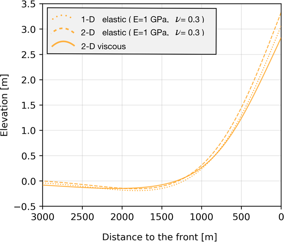
Fig. 7. Example of elastic and early-stage viscous (t = 0.005 a) rampart-moat for E = 1 GPa, ν = 0.3 and l foot = 50 m.
Taking the viscous simulations as reference points and lowering the Young's modulus of the 1-D elastic model to E 1−D = 10 MPa produces similar frontal elevations for the two rheologies for a wide range of foot lengths. These similarities are supported by the 2-D elastic simulations, for which the Lamé parameters in Eqns (A9) and (A11) were calculated using Young's modulus E 2−D = 10 MPa and Poisson's ratio ν = 0.3 (Figs 5a–c and 9a). Indeed, 1-D and 2-D elastic rampart elevation geometries are generally consistent, although we note a tendency of the 2-D elastic model to simulate slightly higher and steeper ramparts than the 1-D model for short l foot, while the opposite occurs for longer l foot. This height difference, however, remains below 20% for l foot = 25 −75 m.
The higher ramparts in the 1-D case, for longer feet, can be partially explained by the fact that the analytical solution does not account for the bending of the foot itself; therefore, it tends to overstate the bending of the entire ice shelf, an effect that is exacerbated as l foot increases. Indeed, here we present only the 1-D scenario where l foot is assumed to be small compared to the typical deformation length scale of a floating ice shelf, i.e. the deformation of the foot itself is negligible. This ‘buoyancy length’ is typically given as l w ≡ (B/ρwg) 1/4, where B ≡ f(E, h, ν) is the bending stiffness of the ice and g the acceleration due to gravity (e.g. Vaughan, Reference Vaughan1995). This allows for a physically intuitive solution (Appendix A.2.2). The full analytic solution with a bending foot can be found in the Supplementary Information of Wagner and others (Reference Wagner2014).
The stress distribution for the 2-D elastic finite element model for different underwater ice feet reveals an instantaneous upward bending bringing the ice shelf to hydrostatic equilibrium (Fig. 8); this is in contrast with the delayed bending in the viscous model. Similarly to the results from the 2-D viscous model, the maximum stress position of the elastic model,....moves closer to the front with increasing foot length (Fig. 9b). This shift of the stress is predominantly a consequence of the relative impact of the water pressure at the ice front, rather than of the length of the foot itself. Indeed, the effect of the foot itself can be isolated in the 1-D elastic-beam framework, for which it can be shown that  $x^\ast _{\rm min} = \lpar \pi /2\ \sqrt {2}\rpar l_{\rm w} \approx 186$ m (for ν = 0.3) from the front, with no l foot dependence (Wagner and others, Reference Wagner2014). While h is fixed here, we tested the impact of varying the Poisson's ratio with values ν ∈ [0.2, 0.4] and found that this affects $x^\ast$
 by less than 5%. This is in agreement with the results of Christmann and others (Reference Christmann, Plate, Müller and Humbert2016), who found little effect of a variable Poisson's ratio on the magnitude and position of the maximum tensile stress when using a visco-elastic framework. For the elastic model, therefore, $x^\ast$
 is predominantly a function of the Young's modulus, while for the viscous model it is predominantly a function of l foot. The seaward shift of $x^\ast$
 for the elastic case is due to the increasing magnitude of the upward bending stress with l foot relative to the background downward stress triggered by the ocean pressure at the front. This gives
  $x^\ast \rightarrow x^\ast _{\rm min}$ in the limit of long l foot.

Fig. 8. Elastic (for E 2−D = 10 MPa and ν = 0.3) effective principal stress for an underwater foot of length (a) 0 m, (b) 10 m, (c) 50 m and (d) 100 m. These elastic solutions exhibit the full deformation produced by the buoyancy stress. Only the portion of the ice shelf within 1000 m of the front is shown.
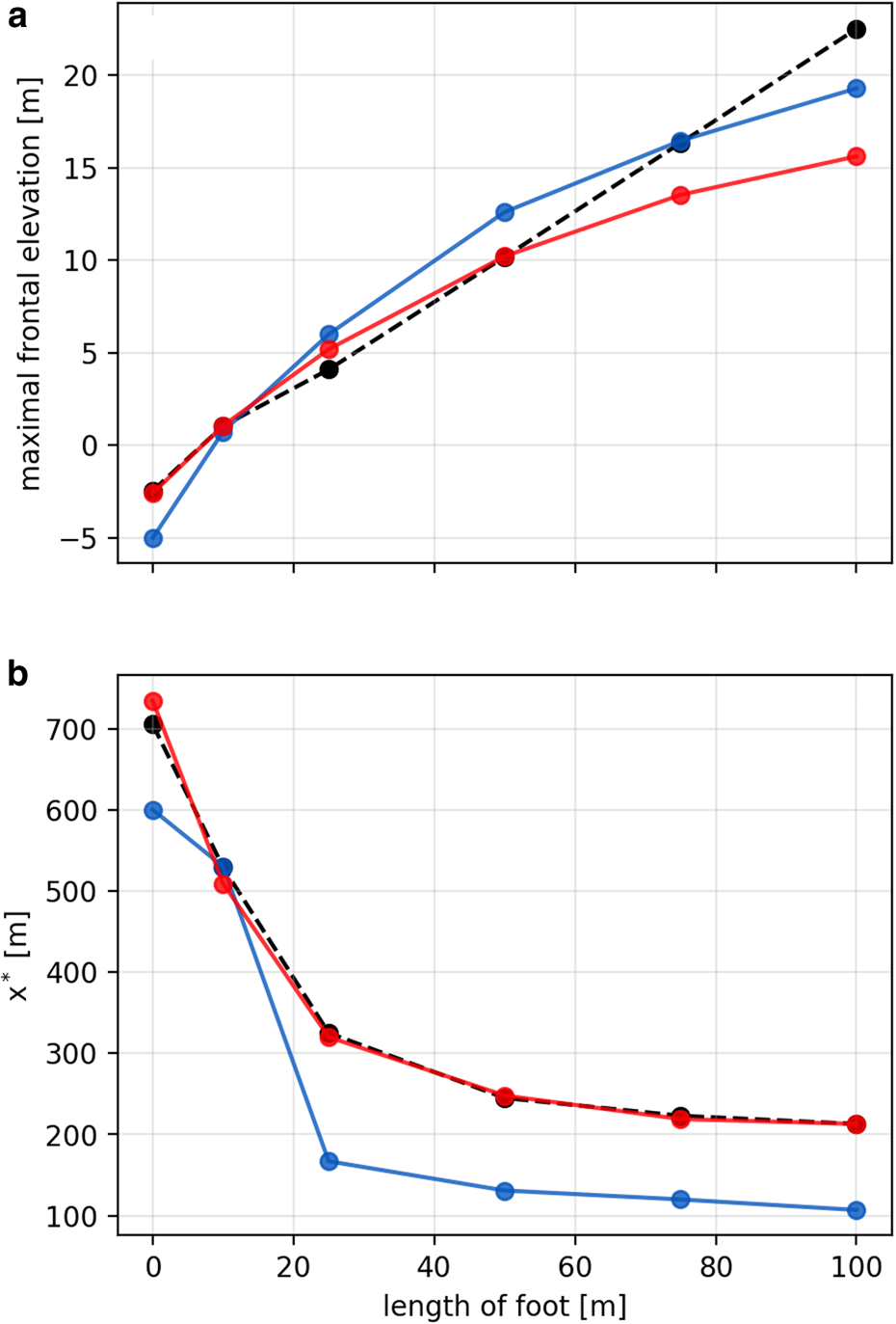
Fig. 9. Comparison between (a) the frontal elevation and (b) the maximum basal stress position x*, with x = 0 representing the ice front, obtained with the viscous (blue), 1-D elastic (for E 1−D = 10 MPa and ν = 0.3; dashed-black) and 2-D elastic (for E 2−D = 10 MPa and ν = 0.3; red) frameworks. The exact numerical values corresponding to the dots are presented in Table 1.
4 Discussion
4.1 The importance of ice rheology
The viscous and elastic frameworks presented here both predict a series of oscillations alternating between areas of extension and compression along the ice-shelf surface due to out-of-plane forcing at the ice edge. The amplitude of oscillation decreases with increasing distance from the front (e.g. Reeh, Reference Reeh1968; Hetenyi, Reference Hetenyi1971; Wagner and others, Reference Wagner2014). Beyond these similarities, the numerical experiments discussed in this study highlight fundamental differences between the two frameworks.
The final rampart-moat geometry formed through viscous deformation is independent of the ice temperature, and thus the ice fluidity. However, the rate of the viscous deformation is regulated by the fluidity of the ice, with the time required for the rampart-moat profile to fully form decreasing as the fluidity increases. That is to say, only the rates of strain and stress change are fluidity dependent, not strain and stress themselves. In contrast, for the elastic rheology, the rampart-moat final geometry forms instantaneously and depends directly on the stiffness of the ice and thus the magnitude of the Young's modulus.
The time-evolving geometry resulting from the viscous framework is associated with a general stress drop in the ice shelf as well as a shift of position of the maximum tensile stress toward the ice front. This is in agreement with the results of Christmann and others (Reference Christmann, Plate, Müller and Humbert2016), who assessed the effect of water pressure on a vertical calving front (i.e. without an underwater foot) and the resulting distribution of stress in an ice shelf. The process is non-linear with a rapid initial decrease in stress and an associated shift of the maximum tensile stress toward the ice front which slows down over time. The length of the foot also affects the rate of deformation of the ice shelf. As a general rule, the longer the underwater foot, the faster the deformation occurs. The exception is for short underwater feet (l foot ~ 10 m), for which the downward-bending effect of the imbalance between ice and water pressure at the ice front is comparable to the net-buoyant forcing created by the foot.
The elastic case is also affected by the downward moment triggered by the water pressure at the ice front, resulting in a negative rampart (i.e. berm) for short underwater feet. The combination of the berm and rampart effects also tends to shift the maximum stress upstream and reduces its magnitude. This effect is particularly notable for short feet, increasing the maximum stress position, x*, by more than 50% for l foot = 25 m with respect to x*min. For l foot = 100 m, by contrast, x* is shifted by only 15% relative to x*min.
As explained in Section 2, the results presented in Section 3 are for an ice density of 850 kg m−3; this is closer to the column-averaged density we observe at ice fronts than the density of pure ice (917 kg m−3), which is usually used in ice-sheet models. Increasing the density from 850 to 917 kg m−3 reduces the rampart-moat elevation as well as the maximal bending stress in both the elastic and viscous frameworks. This is explained by the reduction in the buoyancy of the foot due to the increase in ice density with respect to the density of the water. In the viscous case, the increase in density delays the moment when the rampart-moat reaches its maximum. The position $x^\ast$ also shifts slightly more to the front, contrasting with the elastic case for which an increase in ice density slightly shifts $x^\ast$
 inland.
4.2 Iceberg calving
Our results do not exhibit tensile stresses large enough to surpass the yield stress of pure ice, σy = 1 MPa (e.g. Cuffey and Paterson, Reference Cuffey and Paterson2010). However, the actual yield stress of a crevassed ice shelf can be significantly smaller than this value. According to field observations reported in Vaughan (Reference Vaughan1993) the tensile stress for fracture varies between 0.09 and 0.32 MPa. Similarly, van der Veen (Reference van der Veen1998) considers the value σy = 0.1 MPa sufficient to break already-damaged ice. These values fall in the range of stresses observed in the simulations described above.
We assume that the maximum tensile stress at the base (or surface) of the ice shelf will initiate the opening of an existing crack and eventually lead to calving. If this assumption is correct, the position of the maximum stress can be regarded as the leading parameter to determine the size of calving events. There are two complementary modeling approaches that can take advantage of this statement to forecast the size of a calving event.
Our first approach is to consider the difference in the position of maximum stress, $x^\ast$ , resulting from an elastic framework relative to that of a viscous framework for a fixed forcing, i.e. the same length of underwater foot, l foot. We have shown that in the viscous framework, the maximum stress, $\sigma ^\ast$
 (or its deviatoric part, $\tau ^\ast$
 ), decreases over time and its position, $x^\ast$
 , shifts toward the front. Running a model with a fixed foot geometry would therefore lead to an immediate calving event even before a rampart-moat profile could form. This limitation is due to the foot being imposed suddenly in the model, instead of growing over time. In reality, a gradually growing foot would lead to a buildup of stress over time until it reaches a maximum, σmax, slightly lower than σy but close enough to exceed it at the next small extension of the underwater protrusion. From this point of view, the viscous and elastic models predict calving events of different characteristic sizes. However, this first approach requires that we know the size of the underwater foot. While such information can be collected using underwater sonars (e.g. Wagner and others, Reference Wagner2014, Reference Wagner2019; Sutherland and others, Reference Sutherland2019), it cannot be collected with current airborne and satellite observations (e.g. Scambos and others, Reference Scambos, Sergienko, Sargent, MacAyeal and Fastook2005).
A second approach to predict the size of calving events is to consider an observed rampart-moat surface elevation profile and solve for the length of the foot required to produce this profile in both the viscous and elastic models. Taking the viscous profiles as the reference, we choose a pair of E and l foot values that produces a close agreement between the viscous and elastic rampart-moat profiles. The elastic rampart-moat profiles obtained with E = 10 MPa exhibit surface curvatures that are always smaller than those in the viscous model. We obtain a better correspondence between elastic and viscous profiles when both the Young's modulus and the foot length are decreased. For example, decreasing the Young's modulus to E = 2 MPa and the foot length to l foot = 40 m results in an elastic profile closely aligned with the rampart-moat profile produced by the viscous model with l foot = 50 m (Fig. 5b). In the same way, retaining E at 2 MPa, we find that an elastic profile with l foot = 55 m also best matches a viscous beam with l foot = 75 m, while an elastic profile with l foot = 70 m best matches the viscous model with l foot = 100 m. Overall, for this value of E, the elastic model requires that the foot be about 20–30% shorter than the foot predicted by the viscous model. Similar results are obtained using the 1-D beam model (with E 1−D = 2 MPa). In conclusion, if an observed rampart-moat profile is the result of an elastic deformation it is likely due to a shorter underwater foot and therefore this profile was likely formed over a shorter time than if the deformation was viscous. That is to say, for a given rampart shape, since a shorter underwater foot takes less time to form, and given that stresses are sufficiently high to trigger calving, we expect that these events occur at a higher rate in the elastic framework than in the viscous one.
4.3 Elasticity of ice
The Young's modulus of ice used in our elastic framework is substantially lower than typically referenced in the literature. In various laboratory experiments, the Young's modulus has been found to range from 1 to 10 GPa. Such values have been shown to be too high to reproduce observed rampart-moat profiles (Scambos and others, Reference Scambos, Sergienko, Sargent, MacAyeal and Fastook2005; Wagner and others, Reference Wagner2014). There are several reasons why the Young's modulus could be lower at the ice front: (i) temperature near melting point; (ii) infiltration of seawater at the firn–ice transition; and (iii) crevassing. We consider each of these below.
(i) Temperature near melting point: the 1–10 GPa range was determined for pure ice at low temperatures and under static loading. The elastic modulus has been shown to decrease when strain-rate effects or increases in ice temperature are accounted for, giving rise to the notion of an ‘effective’ Young's modulus (Cuffey and Paterson, Reference Cuffey and Paterson2010). For example, Sinha (Reference Sinha1978) argued that, even for short loading times, E decreases by 20% when the ice is warmed from − 50 to 0°C, and longer loading times can lead to a decrease in E exceeding 50% in their experimental setup. It is thus plausible that ice temperatures close to the melting point, combined with long loading periods (i.e. those associated with slowly forming underwater feet), contribute to a lowering of the effective Young's modulus. This assumption is consistent with findings from Vaughan (Reference Vaughan1995), who demonstrated from a variety of tidal deformation studies that the effective elastic modulus of ice in the vicinity of the grounding line was close to 0.88 ± 0.35 GPa. In another study, Schmeltz and others (Reference Schmeltz, Rignot and MacAyeal2002) have shown that Young's modulus values between 0.8 and 3.5 GPa were needed to correctly simulate temporal changes in tidal flexure of glaciers in both Greenland and Antarctica.
(ii) Infiltration of seawater at the firn–ice transition: the firn–ice transition at the front of some ice shelves is located below the sea surface. In such conditions, seawater can infiltrate the exposed porous firn (e.g. Morse and Waddington, Reference Morse and Waddington1994; Cook and others, Reference Cook, Galton-Fenzi, Ligtenberg and Coleman2018) and increase the fluidity or softness of ice (Duval, Reference Duval1977; Lliboutry and Duval, Reference Lliboutry and Duval1985), to which an effective E may reasonably be related. However, while these explanations could together or separately explain a notable decrease in E, they are unlikely to cause the decrease of two or three orders of magnitude that is required for the fitted elastic solutions above to be physically viable.
(iii) Crevassing: field observations suggest that such low effective Young's moduli are perhaps most likely related to substantial crevassing in the ice shelf. For example, Scambos and others (Reference Scambos, Sergienko, Sargent, MacAyeal and Fastook2005) improved the agreement between observed vertical deflections at the edges of icebergs that had calved from Ronne Ice Shelf and an elastic plate model by significantly lowering the ice thickness. Therefore, a low effective E may be linked to a decreased effective thickness h eff = h − h c, where h c represents a crevassed layer of ice unable to support any bending stress. In this case, the analytical model could be solved using an effective bending stiffness $B_{\rm eff} \equiv Eh_{\rm eff}^3/12\lpar 1-\nu ^2\rpar$
 . This highlights that a given decrease in h eff (i.e. an increase in the maximum crevasse depth) has the same impact on B as a much larger change in E (due to the cubic dependence of B on h), which would explain the small E values needed to fit realistic rampart-moat profiles.

To test this third mechanism, we simulate the effect of elastic buoyancy stresses on an ice shelf with the idealized arrangement of 10 m widecrevasses distributed every 50 m along the ice base. Here, the crevasse depth is taken to extend over 25% of the total ice thickness. We find that such a crevassed ice shelf exhibits a B eff similar to the bending stiffness of a 1-D ice shelf with its thickness set to equal that of h eff in the 2-D case (Fig. 10). The results show that both 1-D and crevassed 2-D models have similar rampart-moat geometries and stress distributions, with the maximum stress position of the two models only differing by ~15%. We only notice a substantially higher tensile stress for the 2-D crevassed ice shelf, but this is mainly linked to the concentration of stress at the tip of the crevasses due to the very low radius of curvature in this area (van der Veen, Reference van der Veen1999).

Fig. 10. (a) Rampart-moat elevation for the 1-D (dotted line) and 2-D (dashed line), (b) deviatoric longitudinal stress at the ice base (τxx; the shaded area represents the 2-D elastic stress, with high spatial variations between crevasse tips and the ice-shelf base, while the dashed line represents a smoothed version of the same stress profile) and (c) effective principal stress (EPS; with a threefold exaggeration of the vertical axis), for E = 1 GPa with a crevassed ice base spanning 25% of the ice thickness (h = 200m), ν = 0.3 and l foot = 50 m. The 2-D case simulates a real crevassed layer while the 1-D case simulates a correspondingly reduced bending stiffness B eff (see text).
The low Young's moduli used in our numerical simulations, while partially supported by the arguments above, are also likely a manifestation of the partially visco-plastic response of the rampart-moat, which limits how well viscous and elastic rampart-moat profiles can match observed shapes for typical Young's moduli, as highlighted by Scambos and others (Reference Scambos, Sergienko, Sargent, MacAyeal and Fastook2005). While fitting an observed rampart-moat elevation with both models will always be possible, the shape and the steepness of the rampart-moat (i.e. the distance between the maximum elevation of the rampart and the position of the minimum of the moat, like it can be measured in Fig. 2) can inform us about the nature and the stage of the deformation. However, in some cases, the use of the 1-D beam elastic model can accurately predict a calving event (Wagner and others, Reference Wagner2014), which makes the elastic 2-D model or its 1-D analytical solution a valuable tool for forecasting a calving event in the context of a rampart-moat.
5 Conclusions and outlook
Motivated by the importance of iceberg calving in ice-sheet mass loss, and by the persistent challenge of finding calving models that reliably forecast the evolution of ice sheets, we have examined the differences between viscous and elastic deformations at the hand of a particular calving process: the footloose mechanism, which is triggered by the formation of an underwater foot at the ice front. We investigated how the ice front responds to stresses from an underwater ice foot using both elastic and viscous frameworks. The two frameworks accommodate these stresses by deforming the ice until it reaches hydrostatic equilibrium, in both cases resulting in a rampart-moat surface profile close to the ice front.
We find that, for a given size of the underwater protrusion (or foot length), the elastic model predicts a maximum stress position that is farther away from the front than the viscous model. This suggests that an ice shelf for which the hydrostatic response to such forcing is predominantly elastic will undergo larger calving events than an ice shelf that is responding through viscous creep. Furthermore, we find that the elastic model reaches a given rampart-moat profile (i.e. a given magnitude of frontal deflection, or given maximum curvature) for a shorter foot than does the viscous model. Because the increase in the size of an underwater foot is mainly determined by the melt rates close to the water surface, this suggests that the time it takes to reach an underwater protrusion triggering the same rampart-moat or strain is shorter for an ice shelf that responds as an elastic solid, compared to one that responds as a viscous fluid. Therefore, in this idealized setup, using an elastic framework for calving will lead to higher calving rates than using a viscous one.
Our results can be extended to any marine-terminating glacier or iceberg that is subject to super-buoyancy mechanisms and rapid deformation. As a pre-calving stress–strain study, our findings are not intended to supply a new way to predict and investigate calving, but rather to highlight the possibly important role that elastic responses may play for certain types of calving events.
While further emphasizing important differences between ice shelves undergoing elastic versus viscous deformations, our findings do not determine which type of response is dominant for most calving events of this type. However, the differences in how the two frameworks achieve calving stresses suggest some areas where further observations may shed light on the dominant rheology: (i) rampart-moat surface profiles, (ii) calving event sizes (measured perpendicular to the ice edge) and (iii) calving frequencies.
In reality, individual calving events will be triggered by a combination of instantaneous, elastic and slow, creeping responses to external forcing. Therefore, looking ahead, comprehensive ice-sheet and calving models would ideally incorporate a visco-elastic account of ice deformation, allowing for both viscosity and elasticity in the ice. This presents a formidable modeling challenge; in the meantime, it will be insightful to further disentangle the relative roles that viscous and elastic responses may play in the calving process.
Acknowledgments
We thank the scientific editor Sergio H Faria, an anonymous reviewer and Julia Christmann for very helpful and insightful reviews. We also thank Matt Trevers for valuable comments and discussions on the original version of the manuscript. This work used the Extreme Science and Engineering Discovery Environment (XSEDE), which is supported by National Science Foundation grant number TG-DPP170004 and TG-DPP190003. The work is part of the National Science Foundation project ROSETTA-Ice, NSF PLR 144353. TJWW was supported by NSF OPP award 1744835.
APPENDIX A. Bending models
For continuously deforming solids and fluids, the equation of state can be written as:

where ρi is the density of ice, $\ddot {{\bi d}}$ the second time derivative of the displacement, $\nabla \cdot$
 is the divergence operator, σ is the Cauchy stress, and g is the gravity. The difference between the two coexisting states for ice, a viscous fluid and an elastic solid, derives from differences in their stress–strain constitutive relations. We describe these two frameworks below.
A.1. Viscous model
The fluid-like framework of ice is typically given in the form of an isotropic power law known as Glen's flow law (Glen, Reference Glen1955), written as

where τ is the deviatoric stress tensor (linked to the Cauchy stress by the equation σ = τ − p I, with p the isotropic pressure and I the identity matrix), η is the effective viscosity, and ${\dot {\bi \varepsilon }}$ is the strain-rate tensor, defined as

Here, the components of the time derivative of the displacement vector ${\dot {\bi d}}$ , $\dot {d}_i$
 , are equal to u i, the components of the velocity vector u. The effective viscosity, η, in Eqn (A2) is given by:

where E A is an enhancement factor, ${{\bi I}_{\dot {{\bi \varepsilon }}}}_2 = \sqrt {{\dot {{\bi \varepsilon }}}_{\bi ij}{\dot {{\bi \varepsilon }}}_{\bi ij}/2}$ is the second invariant of the strain-rate tensor and n is the Glen exponent, with an empirically determined value between 1 and 5 (Weertman, Reference Weertman1983; Gillet-Chaulet and others, Reference Gillet-Chaulet, Hindmarsh, Corr, King and Jenkins2011). An average value of n = 3 is usually used in ice-sheet models and is also used in this study. A is the fluidity, which depends on the temperature following Arrhenius’ law:

with A 0 = 1.258× 10¹³ MPa−3 a−1 (for T < 263 K) and A 0 = 6.046× 1028 MPa−3 a−1 (for T > 263 K) a reference fluidity or prefactor, Q the activation energy, R the gas constant, and T the temperature (in K). Following Cuffey and Paterson (Reference Cuffey and Paterson2010), we set the activation energy to Q = 60 kJ mol−1 for T < 263 K and Q = 115 kJ mol−1 for T > 263 K.
The code is based on a 3-D numerical integration of the Stokes equations – reduced to two dimensions in our case (plane strain) – and computes the ice flow by solving Eqn (A1) – neglecting the inertial term $\rho _{{\rm i}} \ddot {{\bi d}}$ – subject to the principle of mass conservation, ${\bi \nabla } \cdot {\bi u} = 0$
 .
.
For transient simulations, the advection equation of the ice-shelf surfaces is solved to respond to the geometry changes (Gagliardini and others, Reference Gagliardini2013). We apply a Dirichlet boundary condition on the velocity at the ice inflow boundary:

where n is the normal to the surface. Where the ice-shelf surface is in contact with the ocean, we apply a water pressure p w and where the ice-shelf surface is in contact with the atmosphere, we apply a no-pressure condition:

where ρw is the water density, z sl = 0 is the constant sea level and z the altitude where p(z, t) is applied at a time t, resulting in the following Neumann condition applied on the ice–ocean interface:

A.2. Elastic model
A.2.1. Numerical implementation
The linear elastic framework of isotropic ice, undergoing small deformations and assuming stresses below the yield stress of ice, instantaneously links stresses and strains following Hooke's law:

where

and λ and μ are the first and second Lamé parameters, given by:

Here, E is the Young's modulus and ν the Poisson's ratio of ice. The deviatoric stress can then be calculated following

where tr(σ) is the trace of the Cauchy stress.
The elastic displacement of the ice shelf due to ocean forcing can be computed by solving Eqn (A1) subject to Eqns (A9)–(A11). This can be done by working with a structural linear elastic beam, assuming that the external forces act on a 1-D elastic beam. Unsurprisingly, the results are in close agreement with analytical solutions of a conventional 1-D elastic beam (Appendix A.2.2). However, the applicability of this thin-beam approach is limited when considering bending deformations that occur over horizontal scales of a few hundred meters, which is comparable to the thickness of an ice shelf (rather than over horizontal scales that are much longer than the ice-shelf thickness). Therefore, here we use a 2-D (i.e. a flowline section) elastic ice-shelf geometry.
The ocean-pressure loading at the ice base is represented as a nodal force normal to the ice–ocean interface and depends on the ocean pressure at the interface, which evolves as the ice shelf is deflected vertically. This results in the same kind of boundary condition as in the viscous case, given in Eqn (A8). In addition, for low values of Young's modulus, we impose a pre-stress on the ice shelf to avoid excessive compression of the ice shelf and to ensure that the dominant mode of deformation is out-of-plane. We do this by finding a longitudinal pre-stress σps that satisfies the following constraint for the average longitudinal displacement of the beam centerline (i.e. at y = z s − h/2, with zs the surface of the ice shelf and h the ice thickness):

with σps approaching zero for high values of Young's modulus. This can be interpreted as a numerical analog to the analytical method of solving the 1-D equations with a Lagrange multiplier to ensure inextensibility of the beam (Gelfand and others, Reference Gelfand, Fomin and Silverman2000). The numerical implementation of this dynamic process is described in Appendix A.3. Finally, we note that for the inflow condition, in contrast to the viscous case, the elastic case does not rely on any flow computation, and the upstream position of the ice shelf is simply fixed as an embedded beam, following a Dirichlet boundary condition:

A.2.2. Analytical solution
For a floating 1-D elastic beam in steady state (i.e. $\rho _{{\rm i}} \ddot {{\bi d}} = 0$ ), the system described by Eqns (A1) and (A9)–(A11) can be written as (Mansfield, Reference Mansfield2005; Vella and Wettlaufer, Reference Vella and Wettlaufer2008):

where B ≡ E h 3/12(1 − ν2) is the bending stiffness of the beam, w(x) is the height of the beam centerline above the water surface (which corresponds to dz(x) up to a constant). Here, x gives the horizontal distance along the beam, with x = 0 representing the position of the ice front and x > 0 increasing as we move farther inland. Assuming an underwater foot of length l foot and neglecting the bending of the foot itself, Q = Fδ(0) is the load per unit length arising from the foot at the end of the beam (x = 0), with F = F buoyancy − F gravity = l footgh and δ(0), the Dirac delta function acting at x = 0. Under this loading, the solution to Eqn (A15) is (Wagner and others, Reference Wagner2014)

where $H = \rho _{\rm i}\lpar \rho _{\rm w}-\rho _{\rm i}\rpar /\rho _{\rm w}^2 \lpar h/l_{\rm w}\rpar$ is a scaled, dimensionless thickness of the ice shelf that emerges naturally from the calculation and l w ≡ (B/gρw) 1/4 is the ‘buoyancy length’, which reflects the balance of the beam's stiffness and the loading of hydrostatic pressure.
The effect of the pressure at the ice front can also be calculated following a similar principle. Details of the solution can be found in Wagner and others (Reference Wagner2014). Combining Eqn (A16) and the solution of the pressure effect ensures that the effects of the underwater protrusion and the water pressure at the ice front are accounted for simultaneously.
A.3. Numerical stability of the elastic problem
The evolution of the pressure at the ice–ocean interface as the ice shelf is bent out of the water requires a dynamical analysis of the system. We do so by solving the time-dependent Eqn (A1) and by invoking a virtual time, which allows us to take into account the evolution of water pressure as the beam is deflected (i.e. as the mesh deforms elastically). As a result, the perfectly flat ice shelf, with an already-existing foot, initially starts with an unbalanced configuration. In reality, this foot would grow incrementally and the beam would adjust elastically and progressively to this growth, always staying close to the static (quasi-static) equilibrium.
In this conceptual dynamical system, at the beginning of the simulation (t 0), the ice shelf is perfectly flat, and the normal force corresponding to the water pressure is balanced by the weight of the ice, except at the foot, which is completely submerged and therefore net buoyant. When this system is relaxed, the ice shelf elastically rises up (t 1) and the water pressure drops down. Without damping, and due to the conservation of energy of the system, the ice shelf then sinks down (t2) to a position even deeper in the water column than at the beginning of the simulation. This increases the pressure at the ice–ocean interface, pushing the ice even higher out of the water (t 3) and the process continues, giving rise to an unstable system (Fig. 11a). The stabilization of this system requires the introduction of a viscous damping effect that mutes the oscillations. The element node damping forces are related to the element node velocities by a damping coefficient k damp. An appropriate choice of the damping coefficient ensures that the oscillations stabilize toward a steady-state ice-shelf geometry characteristic of its Lamé parameters (Fig. 11b). A weak coefficient would lead to a system that stabilizes very slowly (under-damping) while an overly strong coefficient would lead to a system with no oscillation and that deforms very slowly (over-damping). With such inappropriate damping coefficients, both systems would therefore be unable to reach a steady-state in a reasonable computing time. We also tested and verified the independence of the solution to reasonable Δt, k damp.

Fig. 11. Conceptual model of an elastic ice-shelf evolution with and without damping.
In addition, we tested the convergence of the numerical linear elastic problem, in the limit of the elastic beam theory, by assessing the convergence of the 2-D numerical solution to the 1-D analytical solution. We conducted simulations of elastic deformation for h = 15, 25, 50, 100, 200, 300 and 500 m in the case of l foot = 0 m, i.e. no foot at the ice front. The results show that the berm (negative) elevations in the 1-D and 2-D models tend to converge when h decreases (Fig. 12a), i.e. as the 2-D shelf tends to satisfy the hypothesis of a 1-D beam. The positions of the maximal stress, $x^\ast$ , at the ice base also converge when the ice thickness decreases (Fig. 12b), although the difference between the 1-D and 2-D models remain small (~1% of difference for h = 15 m against ~6% for h = 500 m). These small differences observed in $x^\ast$
 are also consistent with Figure 9, which shows that $x^\ast$
 remains very similar in both the 1-D and 2-D elastic models for the different values of l foot.

Fig. 12. Comparison between the (a) frontal berm elevation and (b) maximal stress position, $x^\ast$ , at the ice base predicted by the 1-D elastic analytical model (for E 1−D = 10 MPa and ν = 0.3; black) and the 2-D elastic model (E 2−D = 10 MPa and ν = 0.3; red), for different values of ice thickness h and l foot = 0 m.


 Open access