Superstabilization of Descriptor Continuous-Time Linear Systems via State-Feedback Using Drazin Inverse Matrix Method


Faculty of Electrical Engineering, Bialystok University of Technology, Wiejska 45D Street, 15-351 Bialystok, Poland
Symmetry 2020, 12(6), 940; https://doi.org/10.3390/sym12060940
Submission received: 5 May 2020
/
Revised: 25 May 2020
/
Accepted: 30 May 2020
/
Published: 3 June 2020
Abstract
:In this paper the descriptor continuous-time linear systems with the regular matrix pencil are investigated using Drazin inverse matrix method. Necessary and sufficient conditions for the stability and superstability of this class of dynamical systems are established. The procedure for computation of the state-feedback gain matrix such that the closed-loop system is superstable is given. The effectiveness of the presented approach is demonstrated on numerical examples.
1. Introduction
Many of the dynamical systems require mathematical model represented by a combined set of differential and algebraic equations. The latter usually refer to constraints imposed on the system in a natural way, resulting from physical laws (e.g., the law of conservation of energy) or defined by the designer (e.g., constrainted motion of the object related to its area of work).
The considered class of systems has different nomenclature in the literature. They are usually called descriptor systems [1], singular systems [2], generalized state-space systems [3] or differential-algebraic equations (DAEs) [4]. In this paper we will use the term “descriptor systems”.
The history of descriptor systems dates back to the 19th century. In 1868 Weierstrass laid the foundations for this theory considering elementary divisors of regular matrix pencils [5], which was then generalized by Kronecker in 1890 for singular pencils [6]. These problems were also investigated by Gantmacher in his monograph in 1959 [7].
A matrix pencil is a set of matrices of the form , where is a parameter and A, B are matrices of the same size. Regularity of the matrix pencil guarantees the existence and uniqueness of the solution to the state equation of the considered class of dynamical systems [1,8]. The pencil is said to be regular if A, B are square matrices and .
The descriptor systems theory flourished in the second half of the 20th century. In 1958 Drazin introduced a generalized inverse of a square matrix [9], which was used in 1976 by Campbell et al. to derive the solution to the state equation of the descriptor continuous-time linear system [10]. Other forms of the solution were obtained by: Rose in 1978 using the Laurent series expansion [11], Yip and Sincovec in 1981 using the Weierstrass–Kronecker canonical form [12]. In subsequent years, lots of papers on analysis and design of descriptor systems were written.
There are many applications of the descriptor systems theory such as analysis of electrical, mechanical and multibody systems as well as modelling of problems in robotics, fluid mechanics, chemical engineering, economy and demography, see, e.g., [1,13,14,15,16,17,18]. Some of complex systems require hybrid models, which are not only based on ordinary differential equations (ODEs) [19].
An overview of state of the art in descriptor systems theory is given in [1,2,8]. Stability of this class of dynamical systems was investigated in [1,8,20,21]. Descriptor closed-loop systems were also studied: with state-feedback [1,8,22], with output-feedback [1,8,23] and with dynamical feedback [1,8,24,25,26]. However, all these works focused mainly on the problems of the pole assignment and regularization of descriptor systems.
Local and global stability criteria for a population model with two age classes were considered in [27]. A special class of stable systems are superstable systems with more restricted dynamics requirements, i.e., with the norm of the state vector decreasing monotonically to zero [28,29,30].
In this paper superstabilization of descriptor continuous-time linear systems via state-feedback using Drazin inverse matrix method will be investigated. The paper is organized as follows. In Section 2, basic definitions and theorems concerning descriptor systems and the Drazin inverse are recalled. The stability and superstability of this class of dynamical systems are discussed in Section 3. In Section 4, descriptor continuous-time linear systems with state-feedback are examined and the procedure for computation of the gain matrix such that the closed-loop system is superstable is presented. Numerical examples and concluding remarks are given in Section 5 and Section 6, respectively.
The following notation will be used: —the set of real numbers, —the set of real matrices and , —the set of complex numbers, —the identity matrix.
2. Preliminaries
In this paper we will consider the continuous-time linear state-space model in the form
where is the state vector, is the input vector and , . The characteristic feature of descriptor systems is that , i.e., the matrix E is not invertible. We distinguish two subclasses of the considered class of systems:
- descriptor systems with the regular matrix pencil , i.e.,
- descriptor systems with the singular matrix pencil , i.e.,
There are several techniques for analyzing the system (1) with (2), e.g., the Laurent series expansion method [11], the Weierstrass–Kronecker decomposition method [12] and the Drazin inverse matrix method [10]. In this paper, we will focus on the last one.
Note that this transformation can be done only for descriptor systems with the regular matrix pencil . Observe that Equations (1) and (4) have the same solution .
Definition 2
The Drazin inverse, like the standard matrix inverse, always exists and it is unique [8,10]. From (7)–(9) it follows that if , then . Some methods for computation of the Drazin inverse are given in [8,31,32].
Lemma 1
Also, the matrices , and can be written in the form
where , is nonsingular, is nilpotent, i.e., for some μ, , and , , .
Let be the set of admissible inputs and be the set of consistent initial conditions for which Equation (1) has a solution for .
Theorem 1
From (14) for we obtain consistent initial conditions for the system
where is an arbitrary vector.
3. Stability and Superstability of Descriptor Continuous-Time Linear Systems
In this section the stability and superstability of descriptor continuous-time linear systems will be discussed. Necessary and sufficient conditions for these properties will be given using Drazin inverse matrix method.
3.1. Stability
In the following considerations it is assumed that , i.e., the descriptor continuous-time linear system (1) has exactly one equilibrium point [8].
Definition 3.
The descriptor continuous-time linear system (1) is called asymptotically stable if
for all consistent initial conditions and .
In contrast to standard dynamical systems (i.e., with ), where we can study their stability based on the eigenvalues of the matrix A, in descriptor systems we analyze the eigenvalues of the matrix pair .
Definition 4.
The characteristic equation of the matrix pair has the form
where and is the characteristic polynomial of the matrix pair .
Theorem 2
Taking into account that Equations (1) and (4) have the same solution , we expect that both models also have the same set of eigenvalues.
Definition 5.
The characteristic equation of the matrix pair is given by
where and is the characteristic polynomial of the matrix pair .
Lemma 2.
The characteristic polynomials of the matrix pairs and are related by
Proof.
The characteristic polynomial of the pair has the form
which is equivalent to (20). □
Note that the characteristic equations of the matrix pairs and have the same form. Therefore, both pairs have the same set of eigenvalues and Theorem 2 can be used for the roots of Equation (19).
The following approach can also be used to test the stability of the descriptor continuous-time linear system (1).
Lemma 3.
The matrix has eigenvalues of the pair (or ) and additionally zero eigenvalues, i.e., its characteristic equation has the form
where is the characteristic polynomial of the matrix .
Proof.
Using (13) we have
since . It is easy to see that and .
Using again (13) we can write
since .
Theorem 3.
Proof.
The proof follows directly from Lemma 3. □
Based on the above considerations we have the following Theorem.
3.2. Superstability
The asymptotic stability of a dynamical system ensures that its free response decreases to zero for , however its value may increase significantly in the initial part of the state vector trajectory. In superstable systems the norm of the state vector decreases monotonically to zero for , which prevents such undesirable effects [28,29,30].
The following norms will be used:
- ∞-norm of a vector
- ∞-norm of a matrix
Definition 6
Quantity is called the superstability degree of the matrix A. If the matrix is superstable, then it is also stable, however the reverse implication does not hold.
Lemma 4
Now let us consider the descriptor continuous-time linear system (1). The solution to Equation (4) (or equivalently (1)) for has the form
Lemma 5.
The matrices and , where is arbitrary, satisfy the equality
Proof.
The matrix can be written in the form
since . □
Using Lemma 5 Equation (34) can be rewritten in the form
where is an arbitrary matrix.
Taking into account (14) and (15) for it is easy to see that if , then . Therefore, from (37) we have
If the matrix is superstable (i.e., it satisfies the condition (31)), then by Lemma 4 we have . From the inequality (38) we obtain
and the norm of the state vector decreases monotonically to zero. Therefore, the following theorem has been proved.
Theorem 6.
The matrix G shall be chosen so that the superstability degree of the matrix takes value higher than zero, i.e., the term eliminates from the matrix unimportant entries that are further canceled through multiplication by .
4. Descriptor Continuous-Time Linear Systems with State-Feedback
In this section descriptor continuous-time linear systems with state-feedback will be examined. The procedure for computation of the gain matrix such that the closed-loop system is superstable will be presented.
First we shall show that Equation (4) can be decomposed into two equations as follows.
Lemma 6.
Let
It is easy to check that the first two components of (14) are the solution to Equation (42) and the third component of (14) is the solution to Equation (43).
4.1. Problem Formulation
Let us consider the system (1) with the state-feedback
where is the new input vector, , are defined by (40) and .
To simplify the notation we introduce
The problem can be stated as follows. Given , , , find K such that the closed-loop system is superstable.
4.2. Problem Solution
Lemma 7.
It is possible to choose the matrix K such that , or , .
The solution to Equation (61) can be obtained using the approach given in [8] and it has the form
where and are the k-th time derivatives of and . Taking into account that
from (64) we have
4.2.1. Stability of the Closed-Loop System
Lemma 8.
Proof.
The proof follows immediately from (66) for , i.e.,
Therefore, if then also . □
Hence, the stability of the closed-loop system (60), (61) depends only on Equation (60), i.e., on the matrix . Thus, we can use the considerations presented in Section 3.1.
Theorem 7.
The descriptor continuous-time linear sysstem (1) with the state-feedback (52) such that is asymptotically stable if and only if one of the following equivalent conditions are met:
- roots of the characteristic equation satisfy the condition (18);
- the matrix has stable eigenvalues and zero eigenvalues.
4.2.2. Superstability of the Closed-Loop System
Theorem 8.
The descriptor continuous-time linear sysstem (1) with the state-feedback (52) such that is superstable if and only if there exists a matrix such that:
- the matrix satisfies the condition (31);
- the inequalityis satisfied.
Proof.
The first condition can be proven in a similar way as Theorem 6, so we will focus on the proof of the second condition. Assume . Using (41), (63) and (67) we have
Let
and
Taking into account (13) and using (71) for (i.e., ) we obtain
where , , . It is easy to check that
since by Lemma 5 it follows that and from (72), (75) we have , . Using (13) and (72)–(76) we obtain
and
Let . The norm of (78) can be expressed by
Thus, for we have . In general case for any matrix T we obtain the condition (68). Note that the matrix G does not change the solution and its choice is arbitrary. The term is used to eliminate unnecessary elements that may occur in the matrix . □
5. Numerical Examples
In this section the effectiveness of the presented approach will be demonstrated on two numerical examples. The first one shows how to test the superstability of the descriptor continuous-time linear system (1) using Theorem 6. The second one shows the procedure for the state-feedback synthesis such that the superstability of the closed-loop system (60), (61) is guaranteed (Theorem 8).
Example 1.
Check the superstability of the descriptor continuous-time linear system (1) with and
It is easy to verify that the matrix pencil is regular, i.e.,
From (5) for we have
The matrix defined by (84) does not satisfy the condition (31). However, using (84) and
we obtain
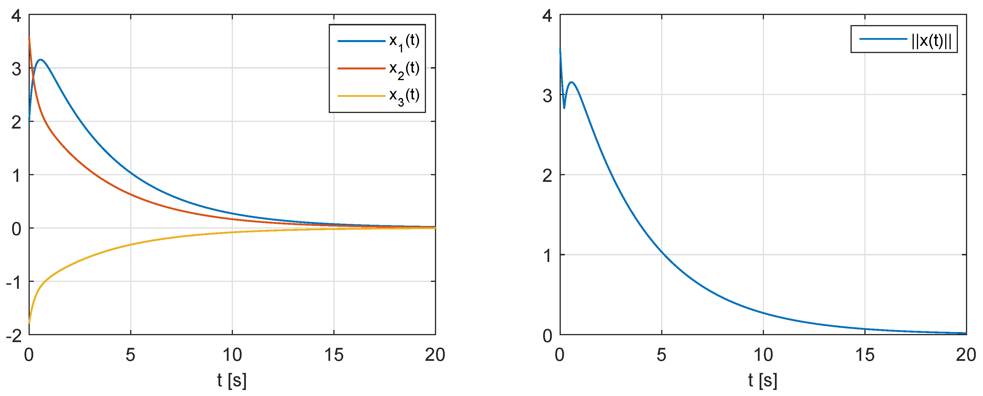
which satisfies (31). Therefore, by Theorem 6 the considered system is superstable. In Figure 1 we present time plots of the state variables and the norm of the state vector for . We can see that the norm of the state vector decreases monotonically for and the system is superstable. Similar result can be obtained for any .
Example 2.
Consider the descriptor continuous-time linear system (1) with
The matrix pencil is regular since
From (5) for we have
Computation of the Drazin inverse of the matrix yields
It is easy to check that there does not exist a matrix such that satisfies (31). Therefore, by Theorem 6 the considered system is not superstable. Now let us consider the state-feedback
where
and
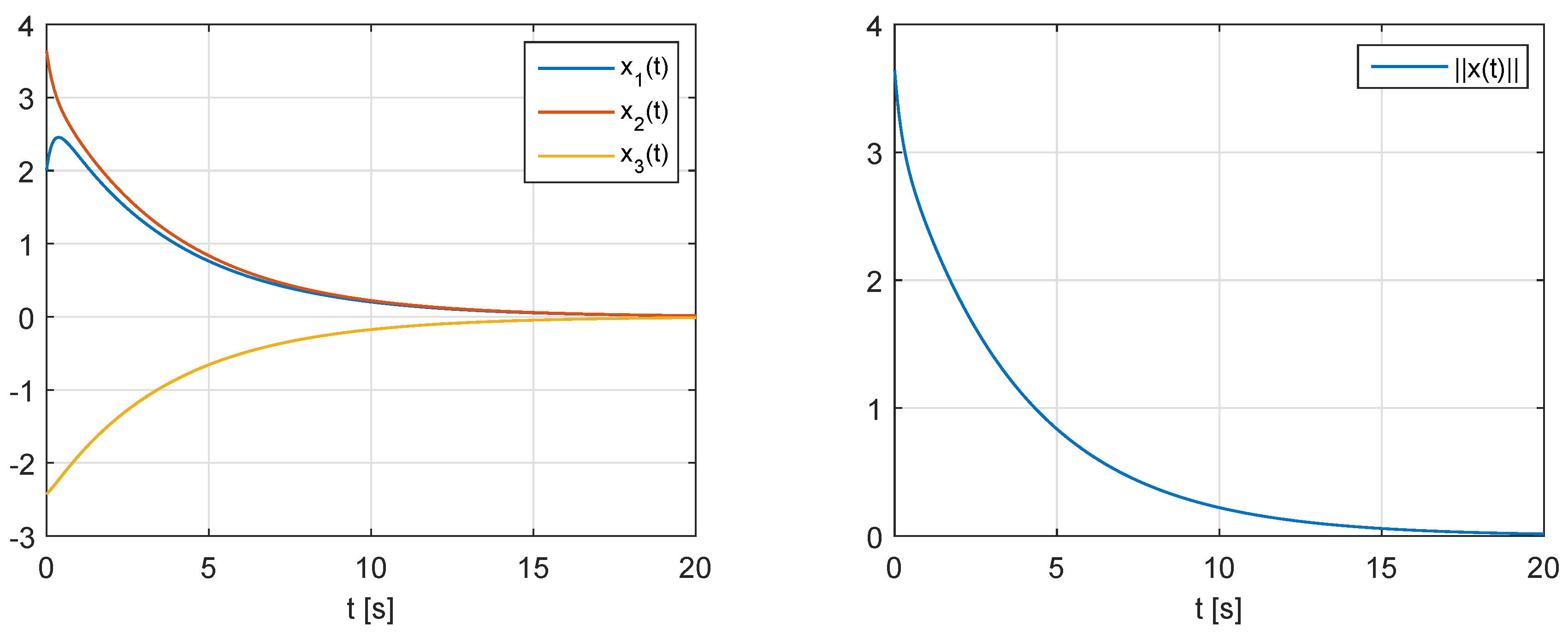
The matrix (98) satisfies (31) and . Therefore, by Theorem 8 the descriptor continuous-time linear system (1), (87) with the state-feedback (92), (95) is superstable. In Figure 2 we present time plots of the state variables and the norm of the state vector for the open-loop system with . We can see that the norm of the state vector does not decrease monotonically for .
In Figure 3 we present time plots of the state variables and the norm of the state vector for the closed-loop system with . Note that the set of consistent initial conditions for the system with the state-feedback is different, i.e., from (69) for and we have for some . After applying the feedback, we can see that the norm of the state vector decrease monotonically for . Similar result can be obtained for any consistent initial conditions .
6. Concluding Remarks
In this paper the descriptor continuous-time linear systems with regular matrix pencil have been investigated using Drazin inverse matrix method and the procedure of state-feedback synthesis such that the closed-loop system is superstable has been proposed.
The presented approach differs from those discussed in the literature, which are mainly focused on the problems of the pole assignment and regularization of descriptor systems, i.e., properties that can be determined basing on the state Equation (1). The method given in the paper allows to design the state-feedback that affects pole-independent system properties such as positivity or superstability for which the standard approach is not applicable. Although a superstable system is also an asymptotically stable one and its poles must have negative real parts, the superstability itself does not depend on the exact location of poles, i.e., from two systems with the same set of stable poles one may be superstable and the other one may not.
The main contributions of this paper can be summarized as follows:
- An alternative method for testing the stability of descriptor continuous-time linear systems has been proposed (Theorems 3 and 4);
- Necessary and sufficient conditions for the superstability of this class of dynamical systems have been established (Theorem 6);
- The procedure for computation of the state-feedback gain matrix such that the closed-loop system is stable (Theorem 7) and superstable (Theorem 8) has been given.
The effectiveness of the presented approach has been demonstrated on numerical examples. The considerations can be extended to fractional-order descriptor continuous-time linear systems.
Funding
This research was funded by National Science Centre in Poland under work No. 2017/27/B/ST7/02443.
Conflicts of Interest
The author declares no conflict of interest.
References
- Guang-Ren, D. Analysis and Design of Descriptor Linear Systems; Springer: New York, NY, USA, 2010. [Google Scholar]
- Dai, L. Singular Control Systems. In Lecture Notes in Control and Information Sciences; Springer: Berlin, Germany, 1989. [Google Scholar]
- Verghese, G.C.; Lévy, B.C.; Kailath, T. A Generalized State-Space for Singular Systems. IEEE Trans. Autom. Control 1981, 26, 811–831. [Google Scholar] [CrossRef]
- Kunkel, P.; Mehrmann, V. Differential-Algebraic Equations. Analysis and Numerical Solution; EMS Publishing House: Zürich, Switzerland, 2006. [Google Scholar]
- Weierstrass, K. Zur Theorie der Bilinearen und Quadratischen Formen. Monatsh. Akad. Wiss. 1868, 311–338. [Google Scholar]
- Kronecker, L. Algebraische Reduktion der Scharen Bilinearer Formen. Sitzungsber. Akad. Wiss. 1890, 763–776. [Google Scholar]
- Gantmacher, F.R. The Theory of Matrices; Chelsea Publishing Company: New York, NY, USA, 1959. [Google Scholar]
- Kaczorek, T. Linear Control Systems. Vol. 1; Research Studies Press, J. Wiley: New York, NY, USA, 1992. [Google Scholar]
- Drazin, M.P. Pseudo-inverses in associative rings and semigroups. Am. Math. Mon. 1958, 65, 506–514. [Google Scholar] [CrossRef]
- Campbell, S.L.; Meyer, C.D.; Rose, N.J. Applications of the Drazin inverse to linear systems of differential equations with singular constant coefficients. SIAM J. Appl. Math. 1976, 31, 411–425. [Google Scholar] [CrossRef]
- Rose, N.J. The Laurent Expansion of a Generalized Resolvent with Some Applications. SIAM J. Math. Anal. 1978, 9, 751–758. [Google Scholar] [CrossRef]
- Yip, E.; Sincovec, R. Solvability, controllability and observability of continuous descriptor systems. IEEE Trans. Autom. Control 1981, 26, 702–707. [Google Scholar] [CrossRef]
- Blajer, W.; Kołodziejczyk, K. Control of under actuated mechanical systems with servo-constraints. Nonlinear Dyn. 2007, 50, 781–791. [Google Scholar] [CrossRef]
- Campbell, S.L. Singular Systems of Differential Equations. In Research Notes in Mathematics; Pitman Advanced Publishing Program: Boston, MA, USA, 1980. [Google Scholar]
- Daoutidis, P. DAEs in chemical engineering: A survey. In Surveys in Differential-Algebraic Equations I. Differential-Algebraic Equations Forum; Springer: Berlin, Germany, 2012. [Google Scholar]
- Kaczorek, T.; Rogowski, K. Fractional Linear Systems and Electrical Circuits. In Studies in Systems, Decision and Control; Springer: Cham, Germany, 2015. [Google Scholar]
- Lewis, F.L. A survey of linear singular systems. Circuits Syst. Signal Process. 1986, 5, 3–36. [Google Scholar] [CrossRef]
- Marszałek, W.; Trzaska, Z.W. DAE models of electrical power systems and their bifurcations around singularities. In Proceedings of the 43rd IEEE Conference on Decision and Control, Nassau, Bahamas, 14–17 December 2004; pp. 4833–4838. [Google Scholar] [CrossRef]
- Martínez-García, M.; Zhang, Y.; Gordon, T. Modeling Lane Keeping by a Hybrid Open-Closed-Loop Pulse Control Scheme. IEEE Trans. Ind. Inform. 2016, 12, 2256–2265. [Google Scholar] [CrossRef] [Green Version]
- Rami, M.A.; Napp, D. Characterization and Stability of Autonomous Positive Descriptor Systems. IEEE Trans. Autom. Control 2012, 57, 2668–2673. [Google Scholar] [CrossRef]
- Virnik, E. Stability analysis of positive descriptor systems. Linear Algebra Appl. 2008, 429, 2640–2659. [Google Scholar] [CrossRef] [Green Version]
- Shafai, B.; Li, C. Positive Stabilization of Singular Systems by Proportional Derivative State Feedback. In Proceedings of the IEEE Conference on Control Technology and Applications, Mauna Lani, HI, USA, 27–30 August 2017; pp. 1140–1146. [Google Scholar] [CrossRef]
- Runyi, Y.; Dianhui, W. Structural properties and poles assignability of LTI singular systems under output feedback. Automatica 2003, 39, 685–692. [Google Scholar] [CrossRef]
- Bunse-Gerstner, A.; Mehrmann, V.; Nichols, N.K. Regularization of descriptor systems by derivative and proportional state feedback. SIAM J. Matrix Anal. Appl. 1992, 13, 46–67. [Google Scholar] [CrossRef]
- Bunse-Gerstner, A.; Mehrmann, V.; Nichols, N.K. Regularization of descriptor systems by output feedback. IEEE Trans. Autom. Control 1994, 39, 1742–1748. [Google Scholar] [CrossRef]
- Chu, D.L.; Ho, D.W.C. Necessary and sufficient conditions for the output feedback regularization of descriptor systems. IEEE Trans. Autom. Control 1999, 44, 405–412. [Google Scholar] [CrossRef]
- Moaaz, O.; Chatzarakis, G.E.; Chalishajar, D.; Bazighifan, O. Dynamics of General Class of Difference Equations and Population Model with Two Age Classes. Mathematics 2020, 8, 516. [Google Scholar] [CrossRef] [Green Version]
- Kaczorek, T. Superstabilization of positive linear electrical circuit by state-feedbacks. Bull. Pol. Acad. Sci. Tech. 2017, 65, 703–708. [Google Scholar] [CrossRef] [Green Version]
- Polyak, B.T.; Shcherbakov, P.S. Superstable Linear Control Systems. I. Analysis. Autom. Remote Control 2002, 63, 1239–1254. [Google Scholar] [CrossRef]
- Talagaev, Y.V. Robust analysis and superstabilization of chaotic systems. In Proceedings of the IEEE Conference on Control Applications, Juan Les Antibes, France, 8–10 October 2014; pp. 1431–1436. [Google Scholar] [CrossRef]
- Kaczorek, T. Extension of Cayley-Hamilton theorem and a procedure for computation of the Drazin inverse matrices. In Proceedings of the 22nd International Conference on Methods and Models in Automation and Robotics (MMAR), Międzyzdroje, Poland, 28–31 August 2017; pp. 70–72. [Google Scholar] [CrossRef]
- Borawski, K. Analysis of the positivity of descriptor continuous-time linear systems by the use of Drazin inverse matrix method. In Automation 2018: Advances in Automation, Robotics and Measurement Techniques; Szewczyk, R., Zieliński, C., Kaliczyńska, M., Eds.; Springer: Cham, Germany, 2018; pp. 172–182. [Google Scholar] [CrossRef]
Figure 1.
State variables (left) and norm of the state vector (right) of the descriptor continuous-time linear system (1) with (80) for .

Figure 2.
State variables (left) and norm of the state vector (right) of the descriptor continuous-time linear system (1) with (87) for .


© 2020 by the author. Licensee MDPI, Basel, Switzerland. This article is an open access article distributed under the terms and conditions of the Creative Commons Attribution (CC BY) license (http://creativecommons.org/licenses/by/4.0/).
Share and Cite
MDPI and ACS Style
Borawski, K. Superstabilization of Descriptor Continuous-Time Linear Systems via State-Feedback Using Drazin Inverse Matrix Method. Symmetry 2020, 12, 940. https://doi.org/10.3390/sym12060940
AMA Style
Borawski K. Superstabilization of Descriptor Continuous-Time Linear Systems via State-Feedback Using Drazin Inverse Matrix Method. Symmetry. 2020; 12(6):940. https://doi.org/10.3390/sym12060940
Chicago/Turabian StyleBorawski, Kamil. 2020. "Superstabilization of Descriptor Continuous-Time Linear Systems via State-Feedback Using Drazin Inverse Matrix Method" Symmetry 12, no. 6: 940. https://doi.org/10.3390/sym12060940
Note that from the first issue of 2016, this journal uses article numbers instead of page numbers. See further details here.