Sliding Modes Control for Heat Transfer in Geodesic Domes
by
 ,
,
Frank Florez
1,*, 
Pedro Fernández de Cordoba
2 ,
,
John Taborda
3,
Miguel Polo
3,
Juan Carlos Castro-Palacio
2 and
María Jezabel Pérez-Quiles
2 1
Faculty of Engineering, Universidad Autónoma de Manizales, Manizales 170003, Colombia
2
Instituto Universitario de Matemática Pura y Aplicada, Universitat Politècnica de València, Camino de Vera s/n, 46022 Valencia, Spain
3
Faculty of Engineering, Universidad del Magdalena, Santa Marta 470003, Colombia
*
Author to whom correspondence should be addressed.
Mathematics 2020, 8(6), 902; https://doi.org/10.3390/math8060902
Submission received: 27 March 2020
/
Revised: 16 April 2020
/
Accepted: 18 April 2020
/
Published: 3 June 2020
(This article belongs to the Special Issue Modeling and Numerical Analysis of Energy and Environment)
Abstract
:The analysis and modeling of unconventional thermal zones is a first step for the inclusion of low-cost spaces and for the assessment of the environmental impact among areas of human use in warm climates. In this paper, the heat transfer in a geodesic dome located at the University of Magdalena (Colombia) is modeled and simulated. The simulator is calibrated against experimental measurements and used to study the effect of different loads which are regulated by a controller in sliding modes explicitly designed for this case. The closed-loop system is used together with ASHRAE Standard 55 to characterize comfort conditions within the dome and the effect on the overall thermal sensation with increasing the number of occupants.
1. Introduction
In the last few decades, the world population has continued growing exponentially. In only 15 years, it increased from 5300 to 7300 million inhabitants, according to the reports of the United Nations. Some models anticipate that in 2030 the world population will be 8500 million. Many countries signed international agreements such as the Kyoto Protocol and the Paris Agreement to fulfil the minimal requirements of the growing population. The crucial objectives are to fight against starvation, poverty, and to provide housing for all the population.
To contribute to the objective of guaranteeing a home for everyone, many researchers have studied different perspectives of human spaces with the focus on reducing the energetic impacts of the current buildings, and looking for new thermal solutions with low energetic consumption. A new strategy to reduce the energy consumption for refrigeration is the reuse of ancient techniques, such as green walls and roof domes among others. Using these structures, the internal temperature of buildings decreases substantially without using heating, ventilation, and air conditioning (HVAC) systems.
Domed roofs are widely used in Middle Eastern countries such as Iran and Turkey [1,2]. These kinds of buildings use the air flux and stratification phenomena to reduce the internal temperature. In works such as [3,4,5], the air flows and their impact on the thermal comfort of the occupants is analyzed and modeled proving that the wind direction plays a significant role in the thermal sensation [6].
Different kinds of domes have been studied to increase the benefits of the domed roofs. Results indicate that the domes receive 30% less of solar radiation than rectangular buildings of similar dimensions [3] and that, for the structure based on triangles, the geodesic domes are the most resistant option [7]. Currently, the geodesic domes are applied in some greenhouses in Canada (Montreal Biosphere) and museums in Geneve [8,9], but their use in Indonesia was especially remarkable after the Jogya earthquake in 2004. This natural disaster generated a tsunami that killed more than 126,000 people in Indonesia alone [10]. Additionally, many people lost their homes and through some programs like “Domes for the World” the victims get assistance by building 80 geodesic domes for residential use [11].
The dome structures are really worth since they can be built very fast and their cost is low. They are really efficient in catastrophic situations. For example, the impact of tornadoes on dome buildings has been widely studied [12]. However, there are many important aspects for further study, such as the thermal modelization of the geodesic domes or the impact of internal loads. This paper presents a mathematical model for a geodesic dome built with the lumped parameter technique. This method introduces new circuit schemes to model non-conventional thermal zones [13].
Thermal models are especially important to reduce the energy consumption, and to guarantee the thermal comfort of buildings in warm climates where the temperatures may be extremely high [14,15]. The use of HVAC systems is widely extended, but the analysis of thermal comfort makes the accurate identification of the real limits and requirements of the thermal zone possible. Another important issue in thermal comfort is the inclusion and selection of a controller for the HVAC system. Predictive control [16] and fuzzy control [17] are methods that have been widely used for this purpose, but it is still necessary to explore alternative controllers, such as sliding modes. This kind of comparative study would help to select the appropriate method in non-conventional thermal zones [18].
In summary, this article presents a mathematical model of a geodesic dome based on a circuit that uses the lumped parameter technique. The geodesic dome is built and monitored to study its thermal comfort requirements and used to adjust the mathematical model. Finally, sliding modes control are presented and tested by introducing cooling and heating internal loads. This paper is organized by sections. In Section 2, the building process of the geodesic dome is presented together with the mathematical model. In Section 3, an evaluation of the experimental data obtained in the dome is given. In Section 4, the adjusting process of the mathematical model and simulator is described. Section 5 introduces the closed-loop model which is analyzed and simulated with different loads. Section 6 presents the conclusions and advances future works.
2. Mathematical Model GDM
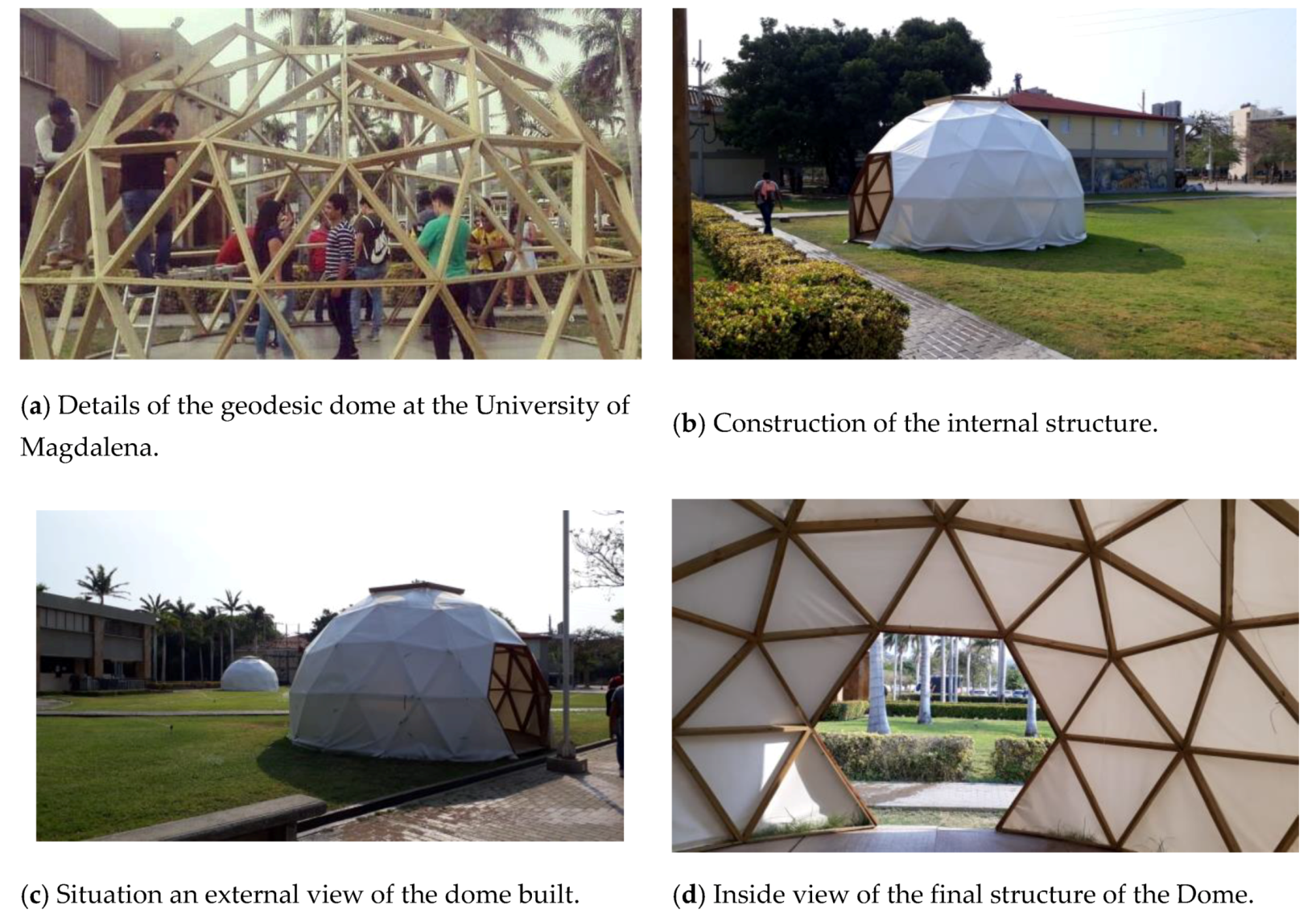
The thermal zones studied in this project are geodesic domes located in the Magdalena University in Santa Marta Colombia. The domes are built by students of the electronic engineering program. In Figure 1, the building process and the final location are shown.
The dome has a diameter of 6 m and a height of m, representing the of the total sphere. It is built with an immunized pinewood skeleton and a polyvinyl chloride (PVC) tarpaulin as an outer shell which has a surface area of m and a thickness of m. The internal structure is organized by triangles of 240 cm × 10 cm × 2.5 cm in 4 rows. In the first two rows, there are 27 triangles, the third was formed with 25 ones, and, in the fourth row, there are only 15 triangles. Additionally, there is a movable crown with five triangles.Thus, a total of 99 triangles for the internal structure are needed giving a surface area of m and a thickness of cm. In Table 1, some physical parameters of the materials are specified, as they are important for the mathematical modelization of the geodesic dome.
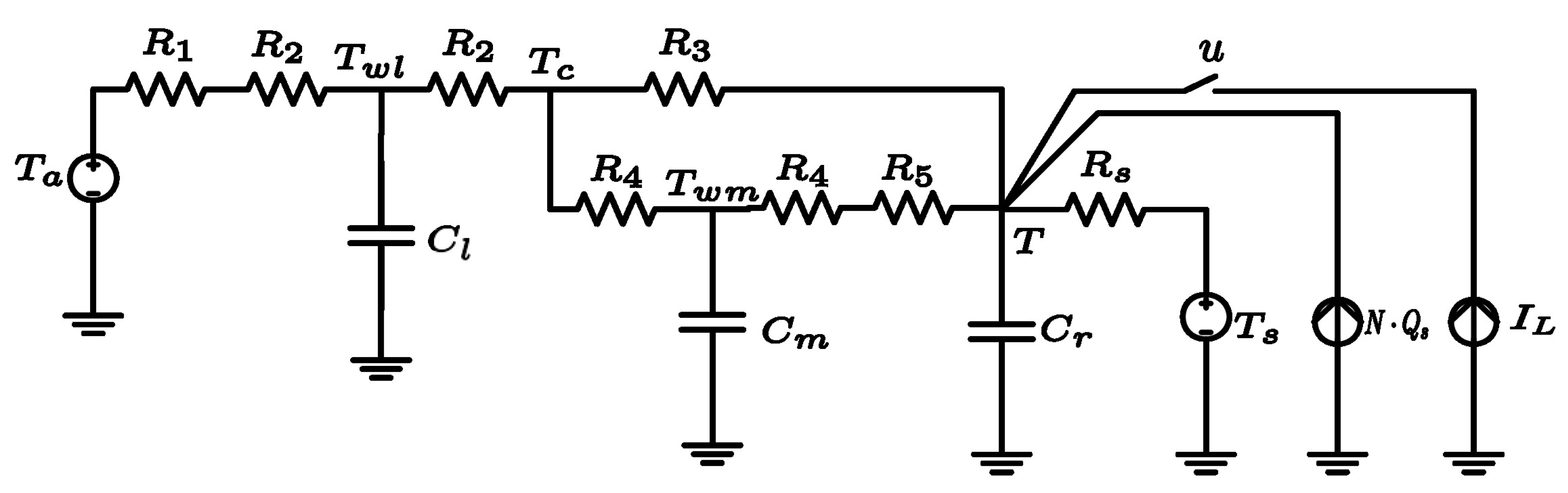
Figure 2 shows the electronic circuit specifically designed for the thermal analysis of the geodesic dome structure, where the resistors and represent the heat transfer between the canvas and the external and internal air, respectively. measures the thermal conduction in the canvas. and represent the heat transfer in the wood by conduction and towards the internal air, respectively. is related to the surface area of the floor and the heat transferred to the internal air. Similarly, , and symbolize the thermal capacity of the canvas, wood, and air to store heat. and are the temperatures of the external air and soil of the dome. Finally, is the temperature of the canvas, of the wood and T of the indoor air.
The magnitudes of the circuit resistors and capacitors are calculated in expressions (1) to (9). In these equations, L, A, and V correspond to the thickness, area and volume of the body, respectively. The parameters k, and are the conductivity, the specific heat and density and the subindices l, m and a symbolize the canvas, the wood and the air, respectively:
To facilitate the simulation and analysis of the dynamic system, the equations are presented with the structure where the vector contains the state variables. This set of equations is called the Geodesic Dome Model or GDM from now on. Finally, the matrices A and B are defined as
The constants to are defined in terms of the circuit resistances and the constant . The constants and include the effect of the ambient and soil temperature. can be modified by adding the term that represents the effect of a cooling internal load and the number of people inside the dome, that is, the occupants. Here, u is the state of the cooling load and the number of occupants:
The expressions
were obtained to determine the equilibrium points of each variable.
3. Register of Environmental Aspects in the Geodesic Dome
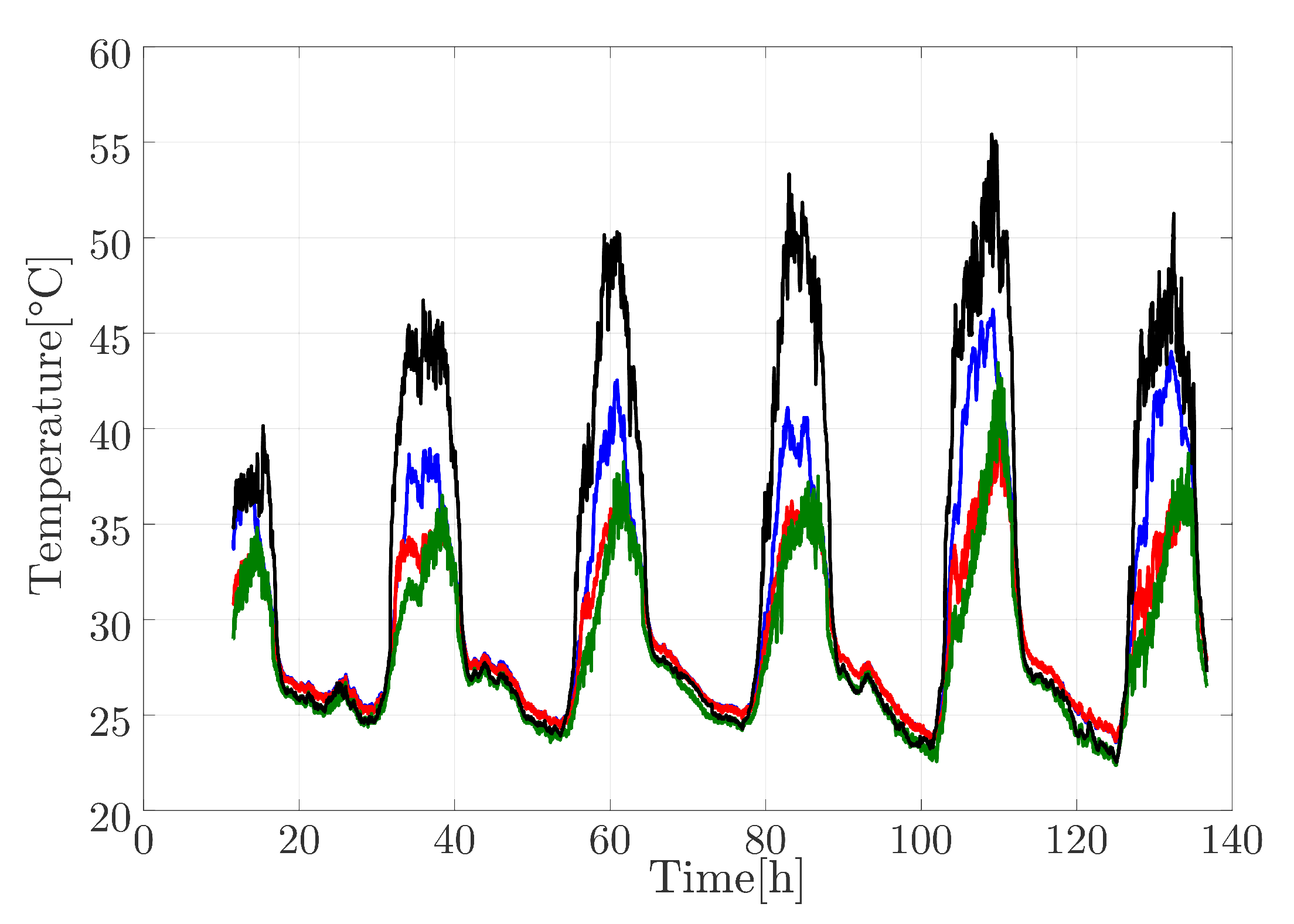
In order to validate our model, all different variables were experimentally measured and registered for five days, from 9 February to 14 February 2019. DS18b20 sensors located in different positions of the internal and external dome cover were used for this purpose and an additional outdoor sensor registered the external temperature. Another sensor in the center of the dome captured the internal temperature.
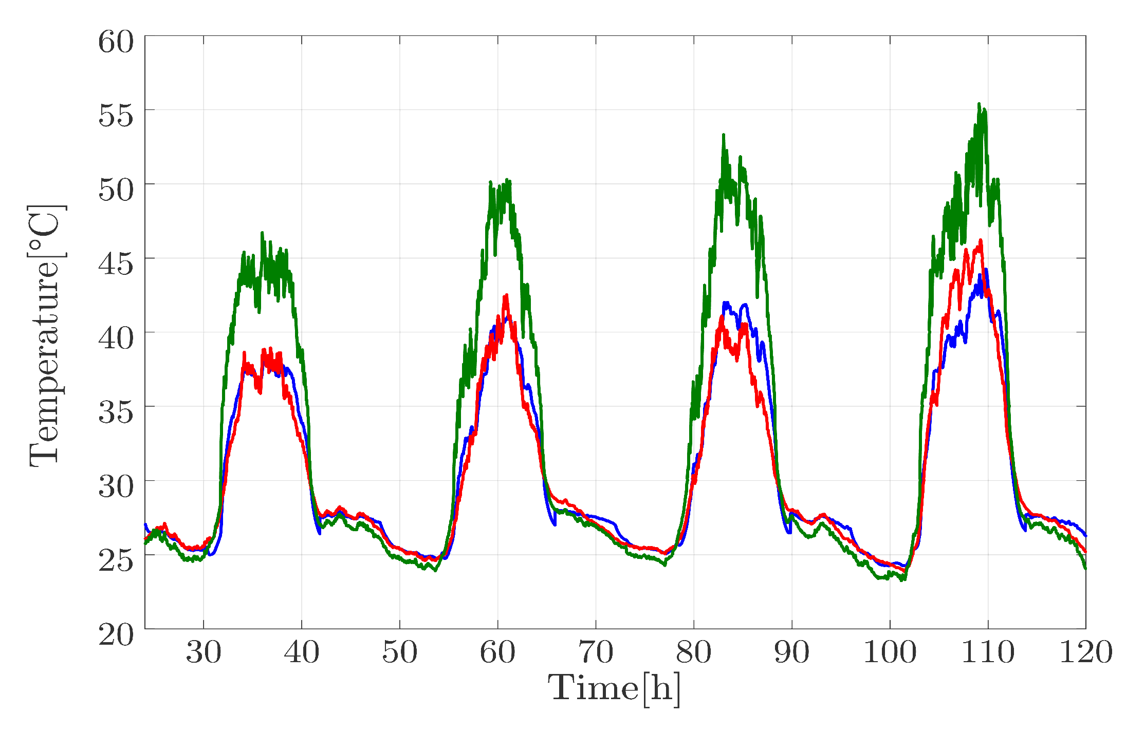
The experimental results are presented in Figure 3 where the blue line indicates the internal temperature, the black line the external temperature, and the red and green lines correspond to internal and external surface temperatures, respectively.
Figure 4 shows the measurements of internal and external surface temperatures, where the red line corresponds to the external sensor and the blue line to the internal one. In these graphs, we can observe that the sensors closest to the door show less difference between the internal and external temperatures probably because of infiltration phenomena.
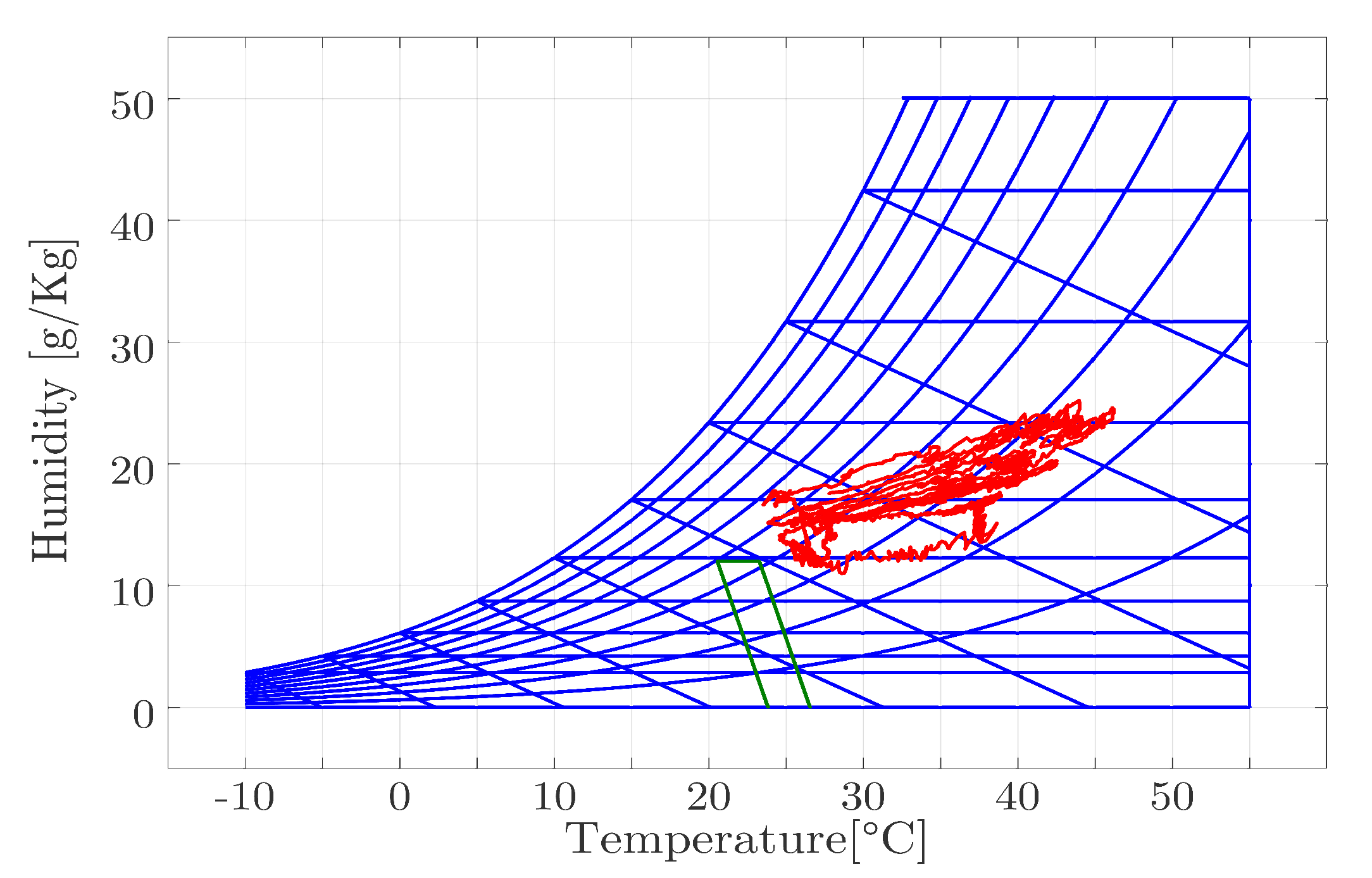
Furthermore, by using the experimental measures, it was possible to understand the cooling needs of the dome. Thermal zone comfort was defined and adjusted using ASHRAE standard 55. This standard considers the thermal insulation by clothing of the occupants, which, for the geographical region, is common for a short-sleeved shirt and pants. This produces an insulation . The temperature limits are adjusted to and . Any other parameters such as ambient humidity and atmospheric pressure are taken from the records of the city of Santa Marta. The comfort zone and the initial conditions in the dome are presented in Figure 5.
4. Simulation of a Geodesic Dome
The recorded experimental data allowed us to do a tuning process to identify the heat transfer coefficients for the structure and outer cover in the canvas. The internal and external coefficients for the wood and the internal coefficients and for the ground were calculated. The structure used to adjust the coefficients is presented in Algorithm 1. This technique requires a vector y with size n for all the heat transfer coefficients. The inputs of the algorithm are contained in two vectors: one for the geometrical and physical parameters of the zone and another one, x, associated to the operating limits for the heat transfer coefficients. The relationship between vectors x and y is expressed as . Internally, the algorithm calculates a period of simulation which in this case is defined by the solar light presence. It is necessary to consider the declination of Earth, , according to the number of days in the year and the coordinates of latitude L. In the final part of the algorithm, an optimization method named OptimToo is performed. This function allows us to evaluate a dynamic system and adjust a set of parameters to minimize an objective function. In this case, the dynamic system is the Geodesic dome model (GDM) and the objective function is the mean square error between the experimental data and the simulation result T. The selection of the optimization method was made after comparing the algorithms of reduction by nonlinear least squares (Lqsnonlin), direct search (PatternSearch), and genetic algorithms (GA). The direct search method was chosen because of its efficiency and speed.
| Algorithm 1: Tuning technique. |
 |
The fine-tuning algorithm was used to calculate the coefficients for diurnal and nocturnal periods. In Table 2, the final values are presented. For diurnal measures, the timing range is 6:20 a.m.–5:50 p.m. and for the nocturnal ones the rest of day.
Based on the model developed, and the coefficients obtained from the tuning algorithm, a simulation was run and the results are presented in Figure 6. In this figure, the red line corresponds to the experimental measurements of the internal temperature, the green line represents the ambient temperature, and the blue line is the model. In this case, the difference between the experimental results and the model was for around 100 h of simulation.
5. Controller Design in Sliding Modes
For the design of the controller, it is necessary to define the state variables of the system. In this case, they are the temperature error, the wood temperature, and the heat flux transferred through the canvas to the internal air
This dynamical system is closed using the equations presented in Section 2. As an example, for the equation of the temperature error, (23), computing the derivative with respect to time one has
Using the open loop definition given in Equation (10), one gets
From the definitions of , and ,
and from here
This last expression can be written as
where the constants are given by
Equations for and are obtained in a similar way. The final structure of the dynamical system is presented in Equation (30):
The constants used in the previous equation are given by
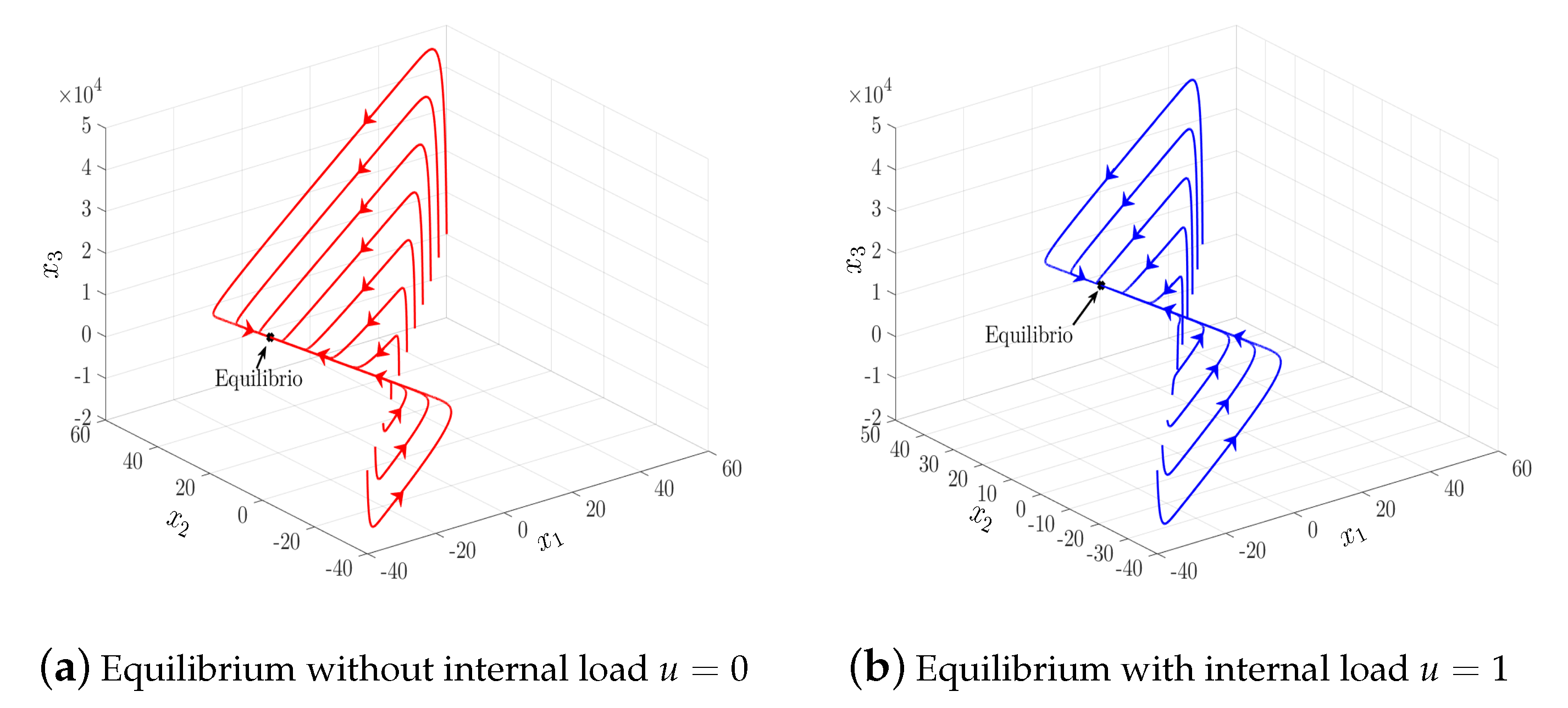
This expression allows us to find the system equilibrium according to the state of the loads. Initially, a heating load with a power of 130 W to represent 1 occupant is introduced and, in a similar way, an ideal cooling load with 12,000 BTU is also introduced. This intensity is typical in a portable HVAC equipment. Based on the dynamical system in closed-loop, it is possible to define equations to calculate the convergence points for each state variable. In Figure 7, the system convergence under constant conditions is verified. For and , the model is simulated with different initial conditions and in all cases the system reaches the steady state at the values predicted by the Equations (39)–(41):
The next step in the controller design is to define the sliding surface. The idea of this algorithm is to employ a certain sliding manifold (surface) as a reference path such that the trajectory of the controlled system is directed to the desired equilibrium point [19]. In Equations (42)–(44), the surface equation and its derivatives are presented. It is possible to build a relationship between the constants. Ideally, the system must be directed to position . At that point, the variable has to be zero. The wood temperature had a low impact on the internal temperature. It can be discarded taking and the incoming heat flux must be minimal. Then, the coefficient of the in Equation (44) is equal to zero by plugging in in Equation (45). Finally, was selected by manual tuning:
The final constants chosen are: , , . The system was simulated with the environmental data recorded and presented in Section 3. The bandwidth was chosen arbitrarily in . The atmospheric pressure is 1017 hPa and the mass constant for the occupants is . The humidity load given of the occupants is calculated with Equation (46):
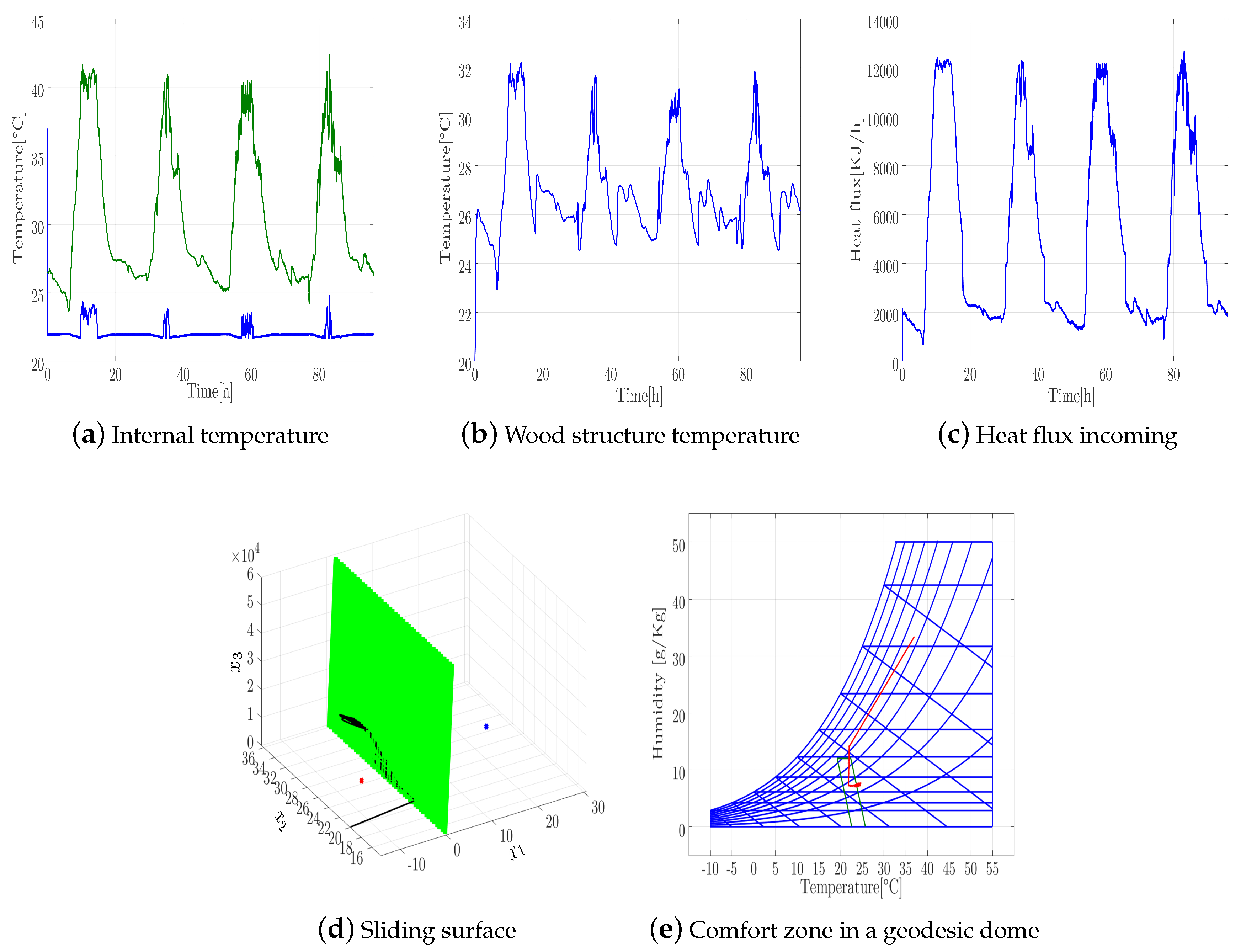
Figure 8 shows the evolution of the system. In Figure 8a, the internal temperature in the dome and the outside temperature are represented by using blue and green lines, respectively. It can be seen that the internal temperature quickly converges to the reference temperature set at , although, during the maximal environmental temperature, it is impossible to be maintained. Figure 8b,c show the evolution of the wood structure temperature and of the incoming flux respectively and, in both cases, the behavior is absolutely dependent on the environmental temperature. Figure 8d shows the sliding surface (green lines) and the points where the equilibrium is reached (blue and red). The black line stands for the surface temperature evolution, and finally Figure 8e shows the psychrometric chart with the comfort zone and the evolution of the humidity and the temperature in the dome. A psychrometric chart is a graphical representation of several thermodynamic properties of air. In this article, we have focused on the two most important ones in terms of comfort, temperature, and humidity. As expected, comfort conditions in the dome were not achieved during periods of maximum outdoor temperature.
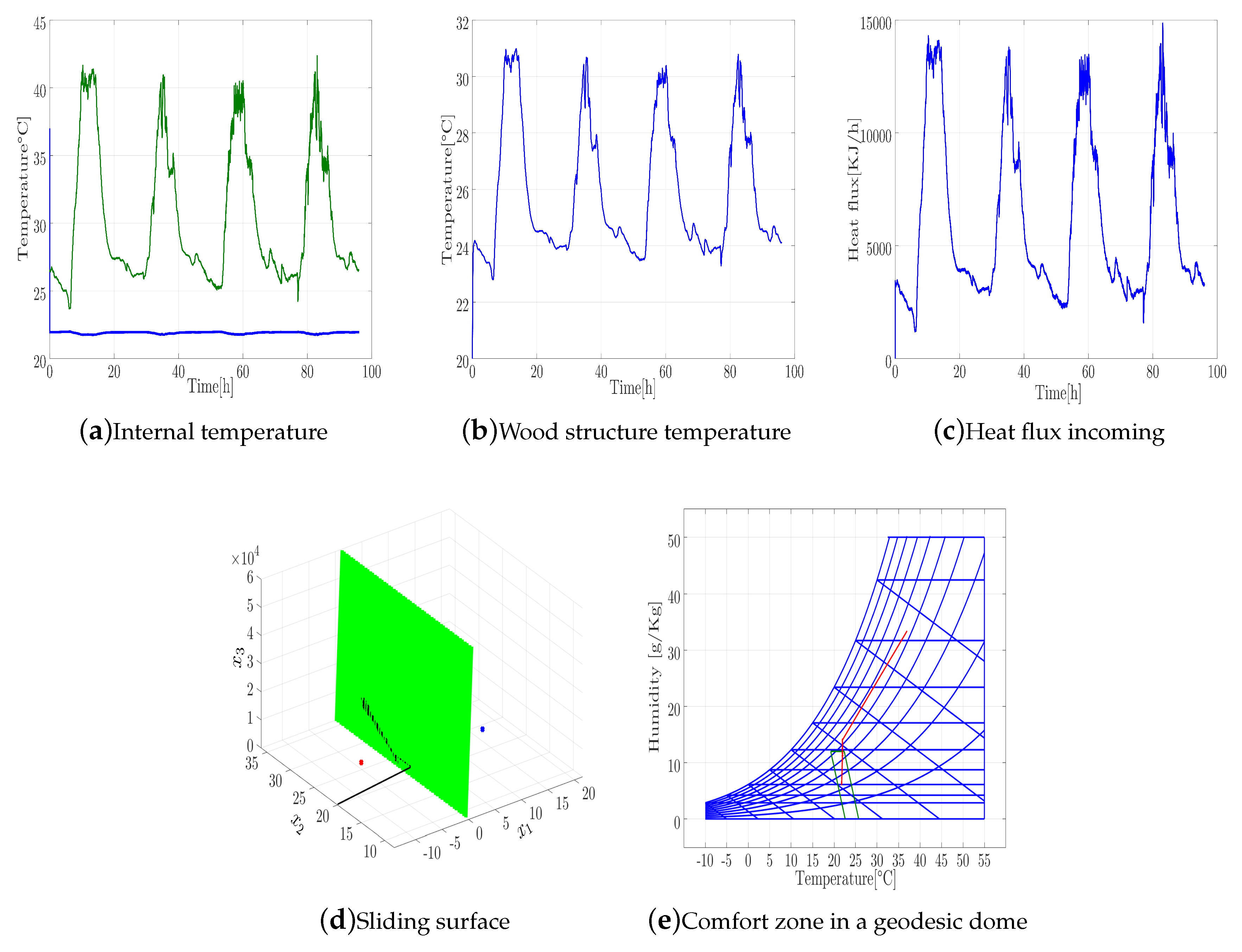
The ideal cooling load was increased to 16,000 KJ to guarantee the comfort zone even during the environmental maximal temperature period. Results are presented in Figure 9. In Figure 9a, the internal temperature of the dome is presented, and it can be seen that the reference of is maintained even during the maximum ambient temperature periods. Similarly, in Figure 9b,c, the temperature of the wood and of the heat flux are presented. Compared with the previous simulation, the wood temperature decreases and the heat flux increases because of the considerable difference of temperature between the exterior and the interior.
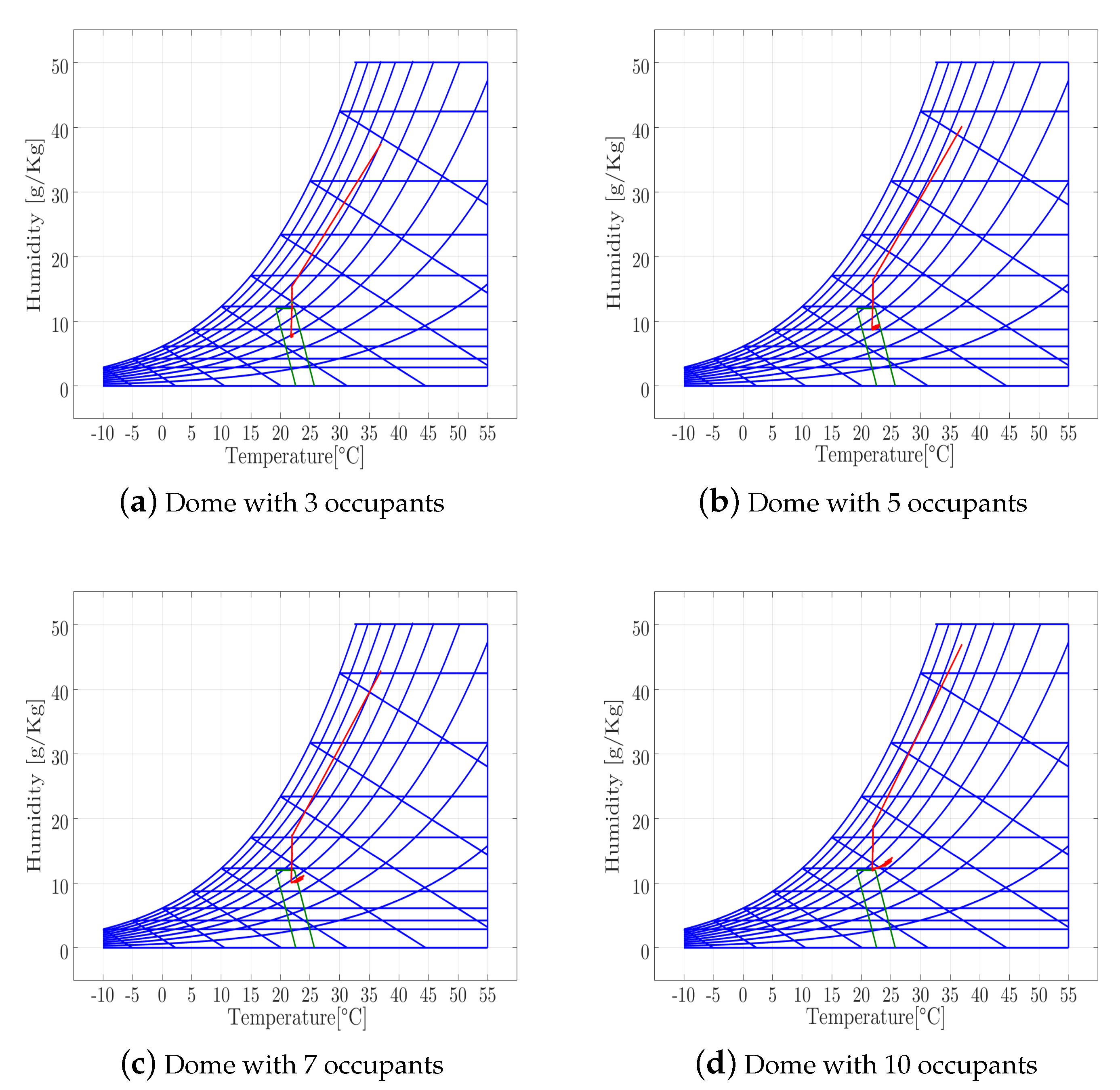
Based on these simulations, it can be concluded that the number of occupants that can support the geodesic dome within comfort levels is 5. Additional occupants may cause the acceptable limits of the comfort standard to be exceeded, making the cooling system insufficient. Figure 10 shows the psychometric charts built with the simulator for different groups of occupants. In Figure 10a, two additional occupants were introduced, but the behavior is very similar to the one presented with only one person inside the dome. In Figure 10b,c, it is shown how the temperature and the internal humidity of the dome increase by the presence of seven occupants instead of five as previously, moving the variables of the comfort zone away. Finally, in Figure 10d, it can be seen that, if the the number of occupants increases to 10, then the conditions of the dome are totally outside the comfort zone.
6. Conclusions
The modeling of unconventional thermal zones is a complex task but can be carried out with the technique of lumped parameters. In this work, an electrical circuit was proposed for representing a geodesic dome located at the University of Magdalena, in Santa Marta (Colombia). A mathematical model considering the dome geometry and its physical characteristics was built up. The experimental conditions of temperature and humidity, both indoor and outdoor, were recorded and used to set up a model. This model reproduces the thermodynamics of the dome with a relative error of .
A controller in sliding modes was designed and simulated, which started from the mathematical model proposed, and allowed for evaluating the effect of introducing cooling and heating loads inside the dome. The comfort conditions were initially studied and then changed. When a refrigerant load of 12,600 BTU was introduced, the power needed was subsequently increased to 16,000 BTU in order to reach the comfort zone defined by ASHRAE Standard 55. Finally, the number of people who admitted the dome without leaving the comfort zone was studied, concluding that, for the simulated conditions, the maximum number of occupants must be five.
Author Contributions
Conceptualization and methodology design: P.F.d.C. and F.F.; experiment development and data collection: J.T. and M.P.; data analysis and simulations: P.F.d.C., F.F. and M.J.P.-Q.; writing—original draft preparation: J.C.C.-P. and M.P.; validation and writing—review and editing: J.C.C.-P. and J.T.; funding acquisition: J.C.C.-P., P.F.d.C. and M.J.P.-Q. The authors consider all of them contributed equally to this work. All authors have read and agreed to the published version of the manuscript.
Funding
This investigation was supported by the national doctoral program of the Colombian Administrative Department of Science Technology and Innovation (Colciencias). P.F.d.C. and M.J.P.-Q. were partially funded by MINECO/FEDER, under project TI2018-102256-B-I00.
Conflicts of Interest
The authors declare no conflict of interest.
Abbreviations
The following abbreviations are used in this manuscript:
| HVAC | Heat ventilation air conditioned |
| GDM | Geodesic dome model |
| ASHRAE | American Society of Heating, Refrigeration and Air Conditioning Engineers |
| BTU | British thermal unit |
References
- Faghih, A.K.; Bahadori, M.N. Three dimensional numerical investigation of air flow over domed roofs. J. Wind Eng. Ind. Aerodyn. 2010, 98, 161–168. [Google Scholar] [CrossRef]
- Saka, M.P. Optimum geometry design of geodesic domes using harmony search algorithm. Adv. Struct. Eng. 2007, 10, 595–606. [Google Scholar] [CrossRef]
- Soleimani, Z.; Calautit, J.K.; Hughes, B.R. Computational analysis of natural ventilation flows in geodesic dome building in hot climates. Computation 2016, 4, 31. [Google Scholar] [CrossRef] [Green Version]
- Khoshab, M.; Dehghan, A.A. Numerical Simulation of Mixed Convection Airflow Under a Dome-Shaped Roof. Arab. J. Sci. Eng. 2014, 39, 1359–1374. [Google Scholar] [CrossRef]
- Faghih, A.K.; Bahadori, M.N. Thermal performance evaluation of domed roofs. Energy Build. 2011, 43, 1254–1263. [Google Scholar] [CrossRef]
- Andrade-cabrera, C.; Rosa, M.; De Kathirgamanathan, A.; Kapetanakis, D.; Finn, D.P. A Study on the Trade-off between Energy Forecasting Accuracy and Computational Complexity in Lumped Parameter Building Energy Models. In Proceedings of the 10th Canada conference of International Building Performance Simulation Association (eSim 2018), Montreal, QC, Canada, 9–10 May 2018; pp. 14–152. [Google Scholar]
- Waghmode, S.; Kulkarni, D.B. Modelling and Validation of Single Layer Geodesic Dome with various Height to Span Ratios. Int. Res. J. Eng. Technol. 2019, 6, 700–706. [Google Scholar]
- Claudino, P. Experimental and Modeling Study of a Geodesic Dome Solar Greenhouse System in Ottawa. Ph.D. Thesis, Carleton University, Ottawa, ON, Canada, 2016. [Google Scholar]
- Pixabay. Switzerland Cern. Available online: https://pixabay.com/en/switzerland-sky-clouds-cern-93275/ (accessed on 30 October 2019).
- Fehr, I.; Grossi, P.; Hernandez, S.; Krebs, T.; McKay, S.; Muir-Wood, R.; Windeler, D. Managing Tsunami Risk in the Aftermath of the 2004 Indian Ocean Earthquake and Tsunami; Risk Management Solutions: Silicon Valley, CA, USA, 2005; p. 124. [Google Scholar]
- Kisnarini, R.; Dinapradipta, A. Improvement Proposal for Dome Houses in Indonesia. In Proceedings of the PLEA 2008 25th Conference on Passive and Low Energy Architecture, Dublin, Ireland, 22–24 October 2008; pp. 22–25. [Google Scholar]
- Li, T.; Yan, G.; Yuan, F.; Chen, G. Dynamic structural responses of long-span dome structures induced by tornadoes. J. Wind Eng. Ind. Aerodyn. 2019, 190, 293308. [Google Scholar] [CrossRef]
- Haghighi, A.P.; Golshaahi, S.S.; Abdinejad, M. A study of vaulted roof assisted evaporative cooling channel for natural cooling of 1-floor buildings. Sustain. Cities Soc. 2015, 14, 89–98. [Google Scholar] [CrossRef]
- Nagarathinam, S.; Doddi, H.; Vasan, A.; Sarangan, V.; Venkata Ramakrishna, P.; Sivasubramaniam, A. Energy efficient thermal comfort in open-plan office buildings. Energy Build. 2017, 139, 476–486. [Google Scholar] [CrossRef]
- He, Y.; Chen, W.; Wang, Z.; Zhang, H. Review of fan-use rates in field studies and their effects on thermal comfort, energy conservation, and human productivity. Energy Build. 2019, 194, 140–162. [Google Scholar] [CrossRef] [Green Version]
- Ryzhov, A.; Ouerdane, H.; Gryazina, E.; Bischi, A.; Turitsyn, K. Model predictive control of indoor microclimate: Existing building stock comfort improvement. Energy Convers. Manag. 2019, 179, 219228. [Google Scholar] [CrossRef] [Green Version]
- Ulpiani, G.; Borgognoni, M.; Romagnoli, A.; Di Perna, C. Comparing the performance of on/off, PID and fuzzy controllers applied to the heating system of an energy-efficient building. Energy Build. 2016, 116, 117. [Google Scholar] [CrossRef]
- Florez, F.; De Córdoba, P.F.; Higán, J.L.; Olivar, G.; Taborda, J. Modeling, Simulation, and Temperature Control of a Thermal Zone with Sliding Modes Strategy. Mathematics 2019, 7, 503. [Google Scholar] [CrossRef] [Green Version]
- Lai, Y.-M.; Tse, C.K.; Tan, S.-C. Sliding Mode Control of Switching Power Converters: Techniques and Implementation; CRC Press: Boca Raton, FL, USA, 2012. [Google Scholar]
Figure 1.
Building the geodesic dome at the University of Magdalena.

Figure 2.
Proposed schematic circuit for a geodesic dome.

Figure 3.
Internal, external, and surface temperatures of the dome.

Figure 4.
Surface temperatures registered at different points of the geodesic dome.

Figure 5.
Psychrometric chart of the geodesic dome in Santa Marta.

Figure 6.
Environmental temperature (green line), internal temperature simulated(blue line), and experimental (red line).
Figure 6.
Environmental temperature (green line), internal temperature simulated(blue line), and experimental (red line).

Figure 7.
Equilibrium of the geodesic dome with and without internal load.

Figure 8.
System variables with a 12,600 KJ cooling system.

Figure 9.
System variables with a 16,000 KJ cooling system.

Figure 10.
Psychrometric chart of a geodesic dome with different occupants.


Table 1.
Thermal parameters of the geodesic dome.
| Material | Specific Heat [] | Density [] | Thermal Conductivity [] |
|---|---|---|---|
| Canvas | 1.0460 | 895.5 | 0.54 |
| Wood | 2.5104 | 640 | 0.756 |
| Air | 1.007 | 1.2 | 0.0864 |
Table 2.
Heat transfer coefficients adjustment.
| Period | ||||
| Day | 140 | 13.75 | 143.25 | 11 |
| Night | 0.0117 | 8.0273 | 100 | 3.2383 |
© 2020 by the authors. Licensee MDPI, Basel, Switzerland. This article is an open access article distributed under the terms and conditions of the Creative Commons Attribution (CC BY) license (http://creativecommons.org/licenses/by/4.0/).
Share and Cite
MDPI and ACS Style
Florez, F.; Fernández de Cordoba, P.; Taborda, J.; Polo, M.; Castro-Palacio, J.C.; Pérez-Quiles, M.J. Sliding Modes Control for Heat Transfer in Geodesic Domes. Mathematics 2020, 8, 902. https://doi.org/10.3390/math8060902
AMA Style
Florez F, Fernández de Cordoba P, Taborda J, Polo M, Castro-Palacio JC, Pérez-Quiles MJ. Sliding Modes Control for Heat Transfer in Geodesic Domes. Mathematics. 2020; 8(6):902. https://doi.org/10.3390/math8060902
Chicago/Turabian StyleFlorez, Frank, Pedro Fernández de Cordoba, John Taborda, Miguel Polo, Juan Carlos Castro-Palacio, and María Jezabel Pérez-Quiles. 2020. "Sliding Modes Control for Heat Transfer in Geodesic Domes" Mathematics 8, no. 6: 902. https://doi.org/10.3390/math8060902
Note that from the first issue of 2016, this journal uses article numbers instead of page numbers. See further details here.