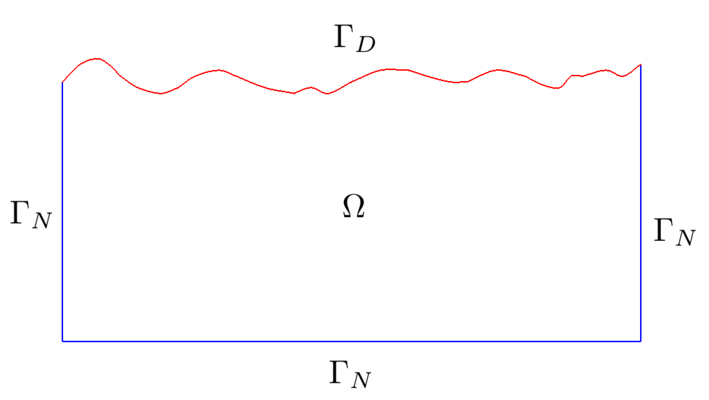
Figure 1.
Computational domain with rough boundaries on the top.
Figure 1.
Computational domain with rough boundaries on the top.
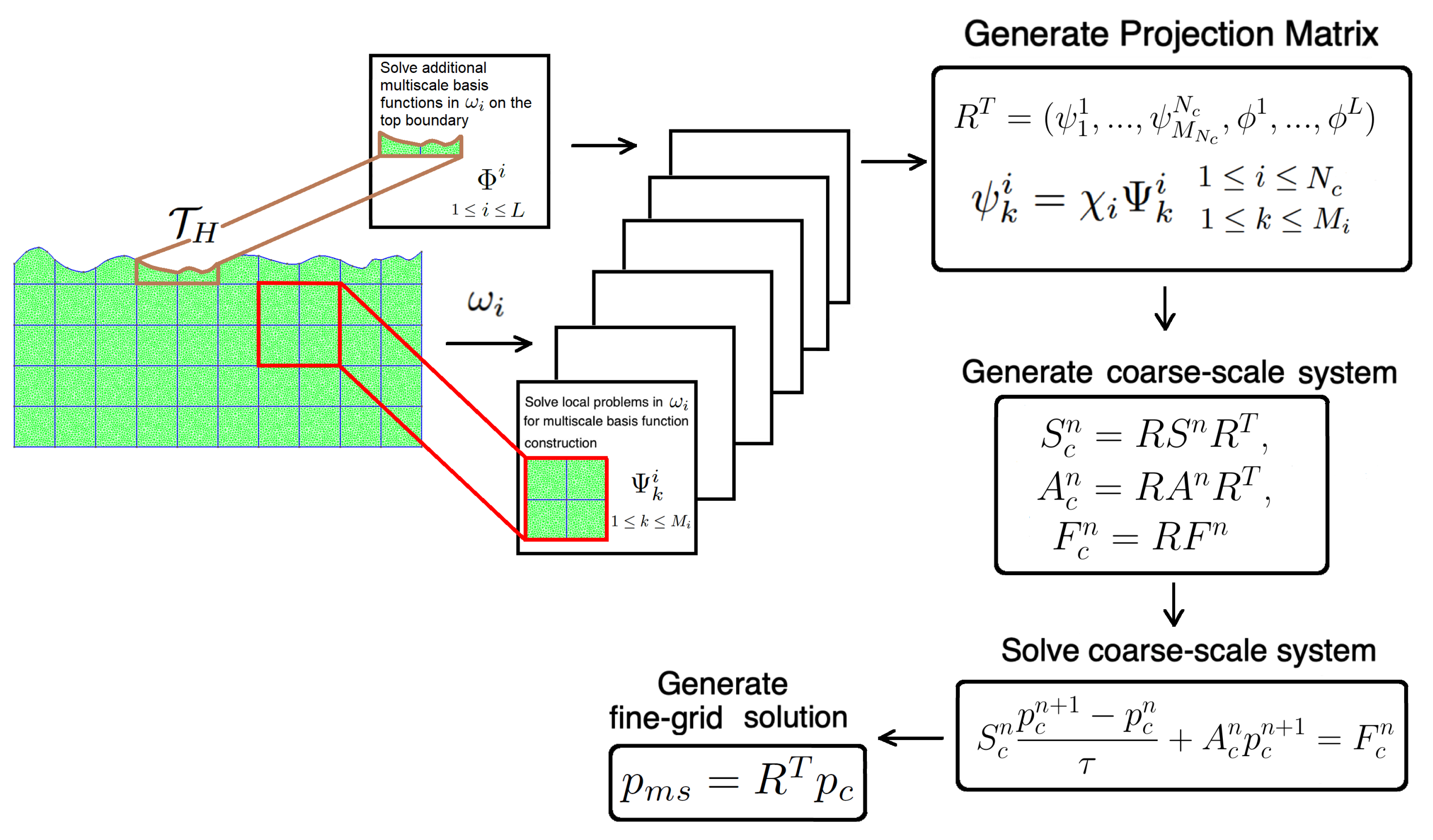
Figure 2.
Illustration of the Generalized Multiscale Finite Element Method (GMsFEM) algorithm.
Figure 2.
Illustration of the Generalized Multiscale Finite Element Method (GMsFEM) algorithm.
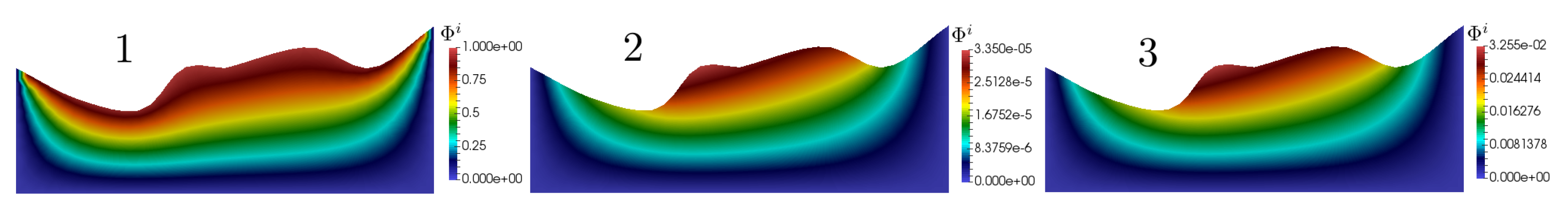
Figure 3.
Illustration of the additional multiscale basis function.
Left: The solution of the problem (
12).
Middle: The solution of the problem (
13).
Right: The solution of the problem (
14).
Figure 3.
Illustration of the additional multiscale basis function.
Left: The solution of the problem (
12).
Middle: The solution of the problem (
13).
Right: The solution of the problem (
14).
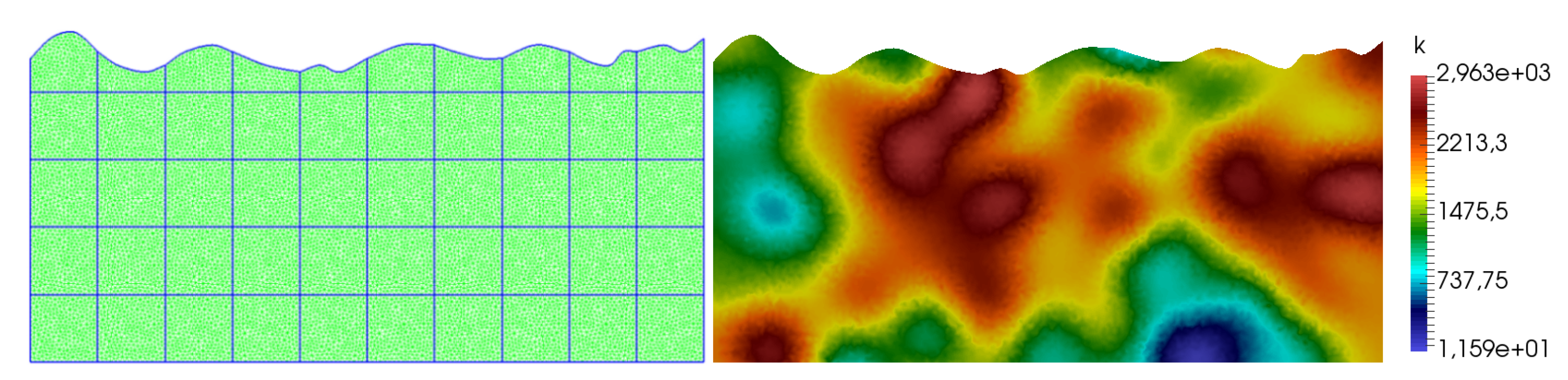
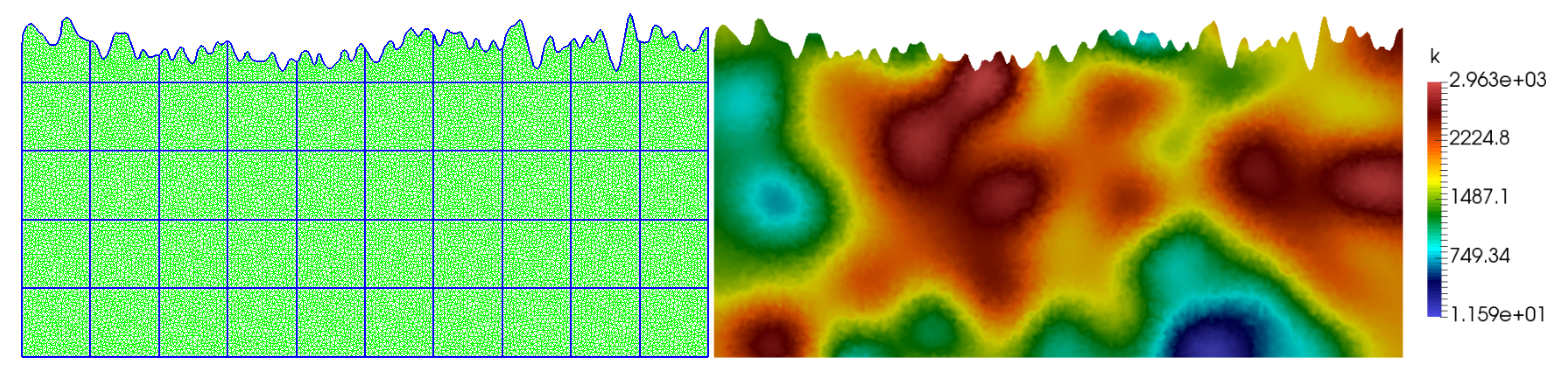
Figure 4.
Computational grids and heterogeneous properties for Tests 1.DBC, 1.NBC, 1.RBC (two-dimensional problem). Left: Coarse grid (blue color) and fine grid (green color). Right: Heterogeneous coefficient .
Figure 4.
Computational grids and heterogeneous properties for Tests 1.DBC, 1.NBC, 1.RBC (two-dimensional problem). Left: Coarse grid (blue color) and fine grid (green color). Right: Heterogeneous coefficient .
Figure 5.
Computational grids and heterogeneous properties for Tests 2.DBC, 2.NBC, 2.RBC (two-dimensional problem). Left: Coarse grid (blue color) and fine grid (green color). Right: Heterogeneous coefficient .
Figure 5.
Computational grids and heterogeneous properties for Tests 2.DBC, 2.NBC, 2.RBC (two-dimensional problem). Left: Coarse grid (blue color) and fine grid (green color). Right: Heterogeneous coefficient .
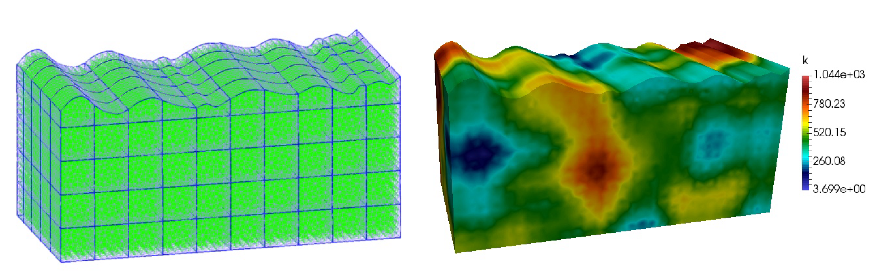
Figure 6.
Computational grids and heterogeneous properties for Tests 3.DBC, 3.NBC, 3.RBC (three-dimensional problem). Left: Coarse grid (blue color) and fine grid (green color). Right: Heterogeneous coefficient .
Figure 6.
Computational grids and heterogeneous properties for Tests 3.DBC, 3.NBC, 3.RBC (three-dimensional problem). Left: Coarse grid (blue color) and fine grid (green color). Right: Heterogeneous coefficient .
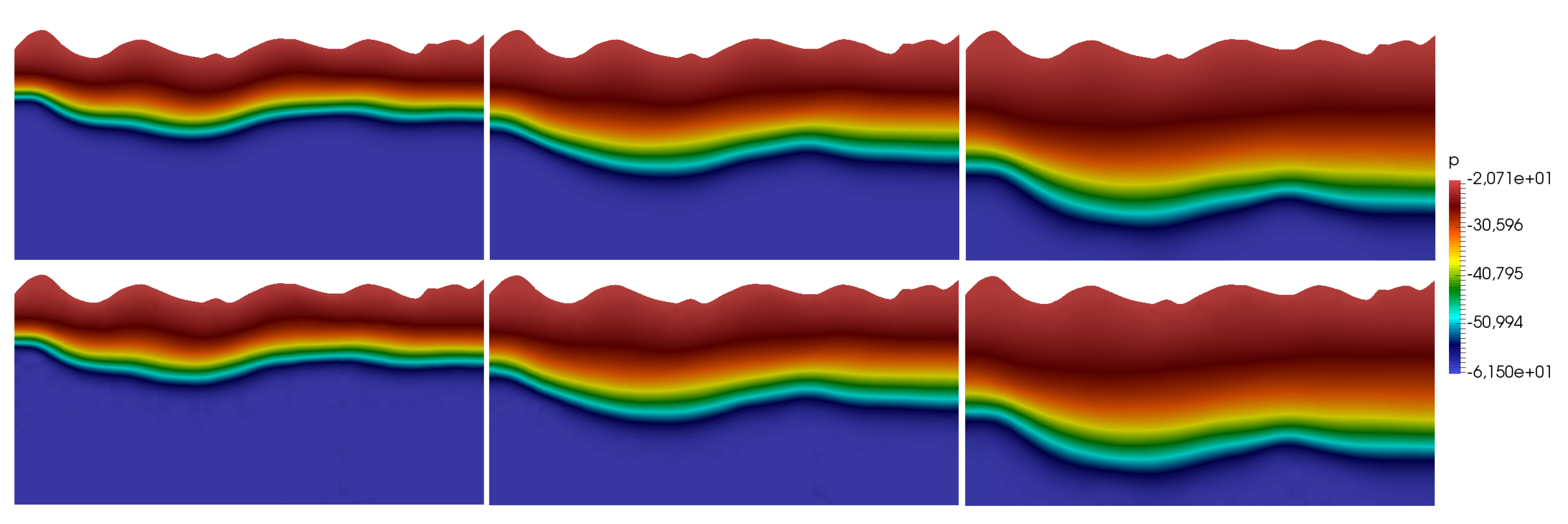
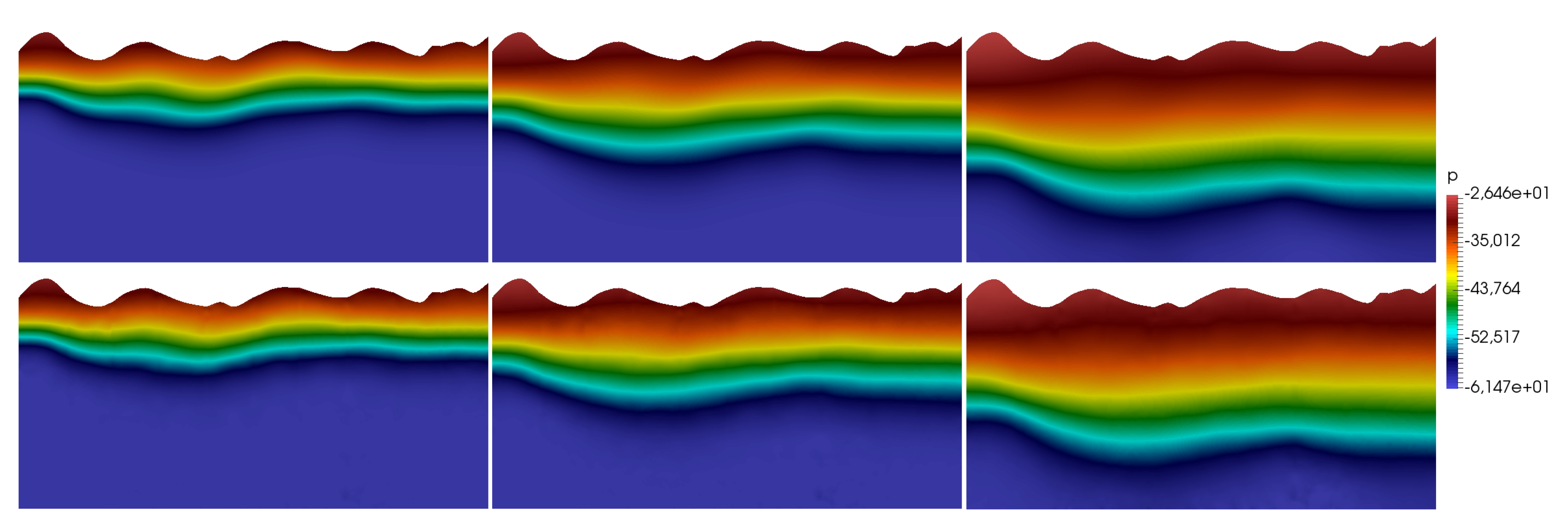
Figure 7.
Numerical results for Test 1.DBC. Solutions p and for different times: , , and (from left to right). First row: Fine-scale solution . Second row: Multiscale solution using 16 basis functions .
Figure 7.
Numerical results for Test 1.DBC. Solutions p and for different times: , , and (from left to right). First row: Fine-scale solution . Second row: Multiscale solution using 16 basis functions .
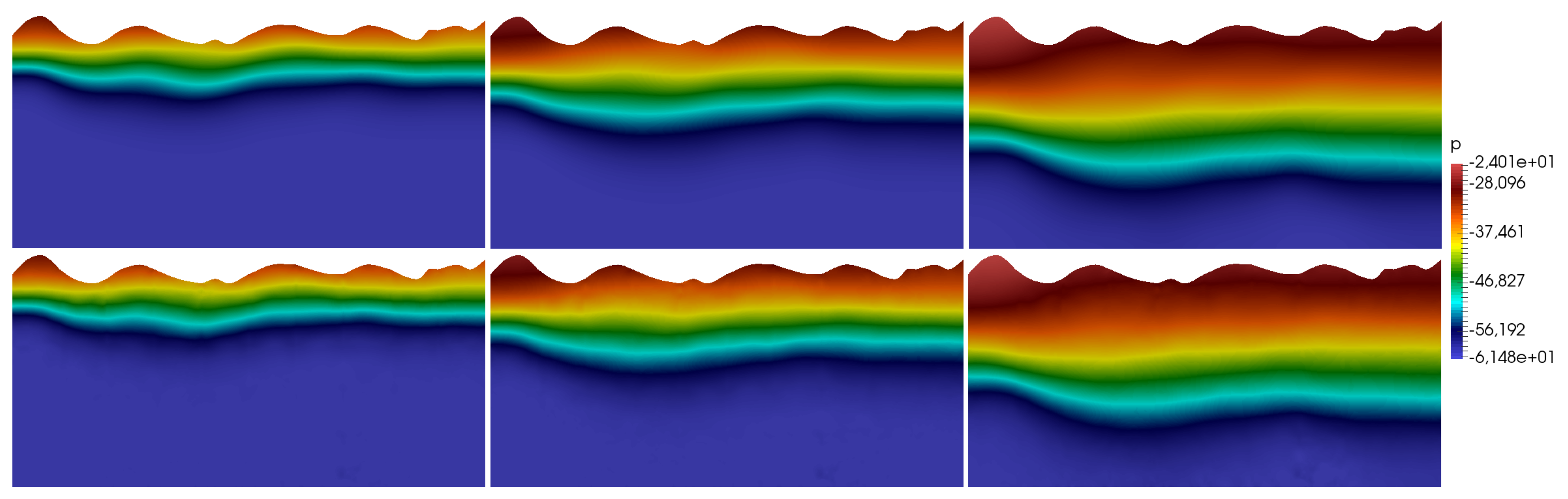
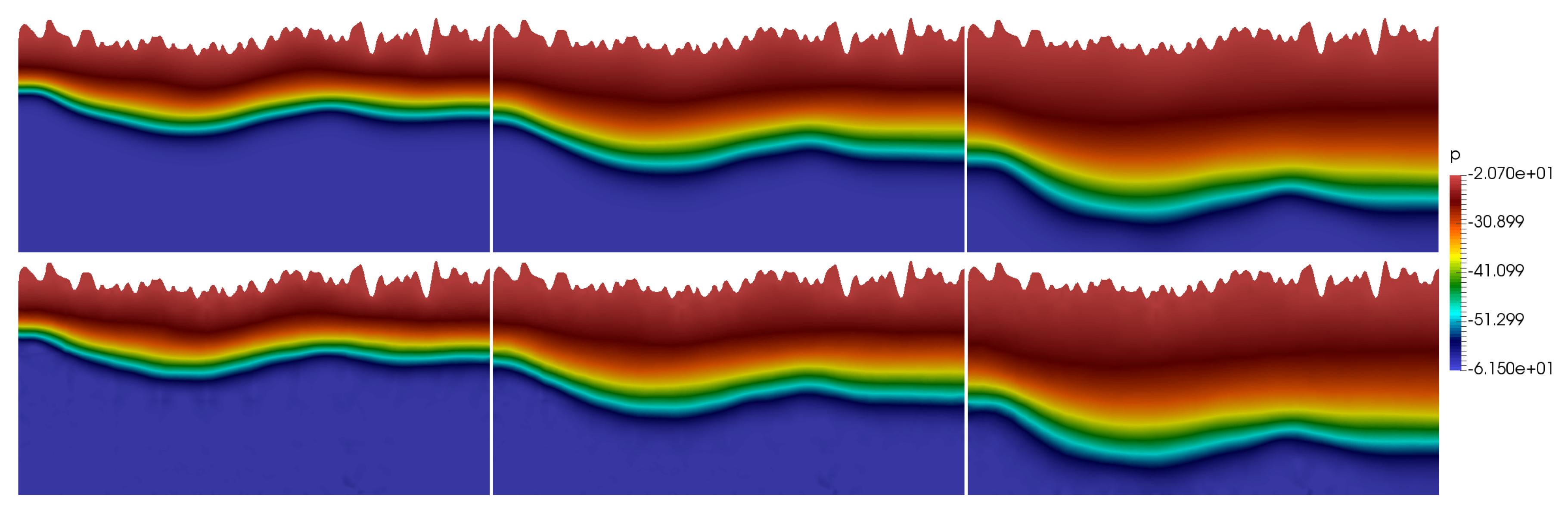
Figure 8.
Numerical results for Test 1.NBC. Solutions p and for different times: , , and (from left to right). First row: Fine-scale solution . Second row: Multiscale solution using 16 basis functions .
Figure 8.
Numerical results for Test 1.NBC. Solutions p and for different times: , , and (from left to right). First row: Fine-scale solution . Second row: Multiscale solution using 16 basis functions .
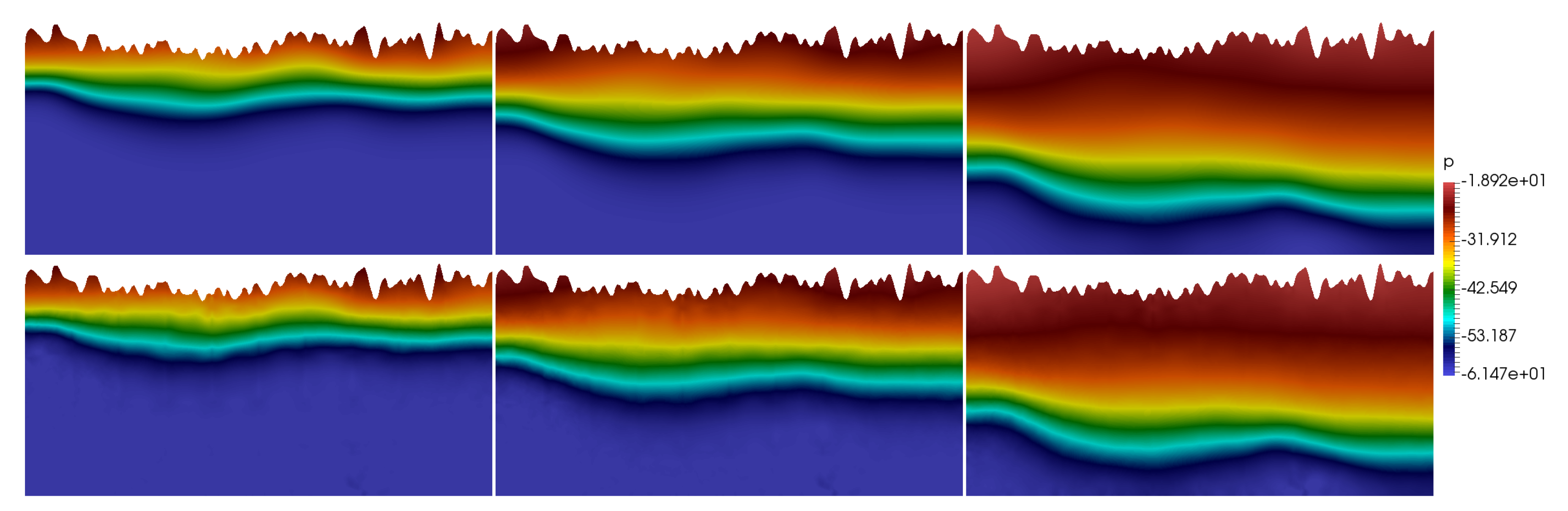
Figure 9.
Numerical results for Test 1.RBC. Solutions p and for different times: , , and (from left to right). First row: Fine-scale solution . Second row: Multiscale solution using 16 basis functions .
Figure 9.
Numerical results for Test 1.RBC. Solutions p and for different times: , , and (from left to right). First row: Fine-scale solution . Second row: Multiscale solution using 16 basis functions .
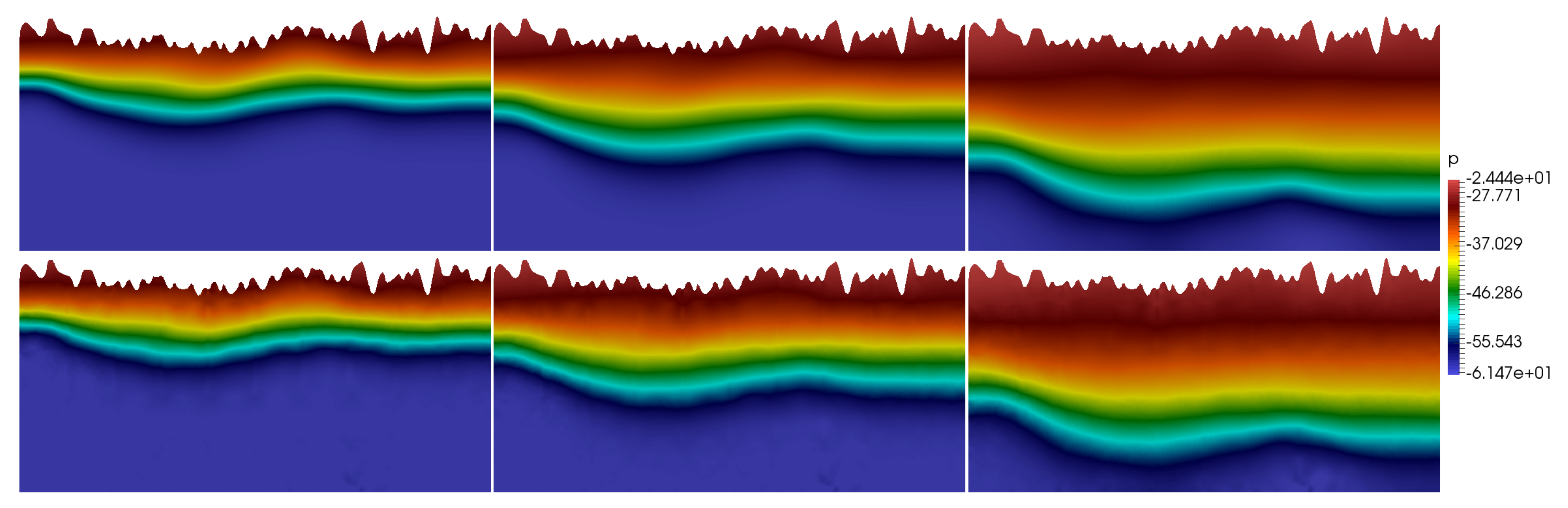
Figure 10.
Numerical results for Test 2.DBC. Solutions p and for different times: , , and (from left to right). First row: Fine-scale solution . Second row: Multiscale solution using 16 basis functions .
Figure 10.
Numerical results for Test 2.DBC. Solutions p and for different times: , , and (from left to right). First row: Fine-scale solution . Second row: Multiscale solution using 16 basis functions .
Figure 11.
Numerical results for Test 2.NBC. Solutions p and for different times: , , and (from left to right). First row: Fine-scale solution . Second row: Multiscale solution using 16 basis functions .
Figure 11.
Numerical results for Test 2.NBC. Solutions p and for different times: , , and (from left to right). First row: Fine-scale solution . Second row: Multiscale solution using 16 basis functions .
Figure 12.
Numerical results for Test 2.RBC. Solutions p and for different times: , , and (from left to right). First row: Fine-scale solution . Second row: Multiscale solution using 16 basis functions .
Figure 12.
Numerical results for Test 2.RBC. Solutions p and for different times: , , and (from left to right). First row: Fine-scale solution . Second row: Multiscale solution using 16 basis functions .
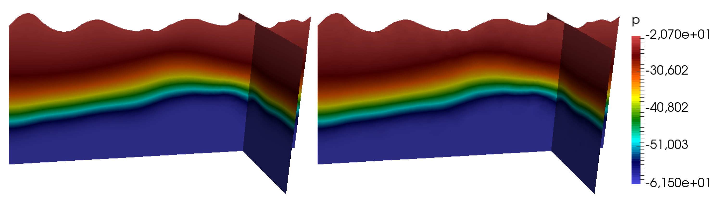
Figure 13.
Numerical results for Test 3.DBC. Solutions p and for the final time. Left: Fine-scale solution . Right: Multiscale solution using 32 basis functions .
Figure 13.
Numerical results for Test 3.DBC. Solutions p and for the final time. Left: Fine-scale solution . Right: Multiscale solution using 32 basis functions .
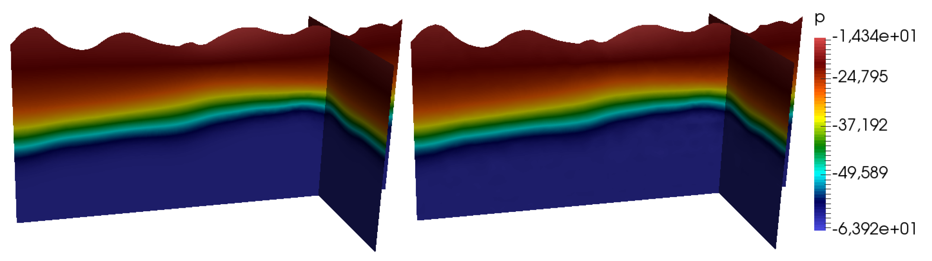
Figure 14.
Numerical results for Test 3.NBC. Solutions p and for the final time. Left: Fine-scale solution . Right: Multiscale solution using 32 basis functions .
Figure 14.
Numerical results for Test 3.NBC. Solutions p and for the final time. Left: Fine-scale solution . Right: Multiscale solution using 32 basis functions .
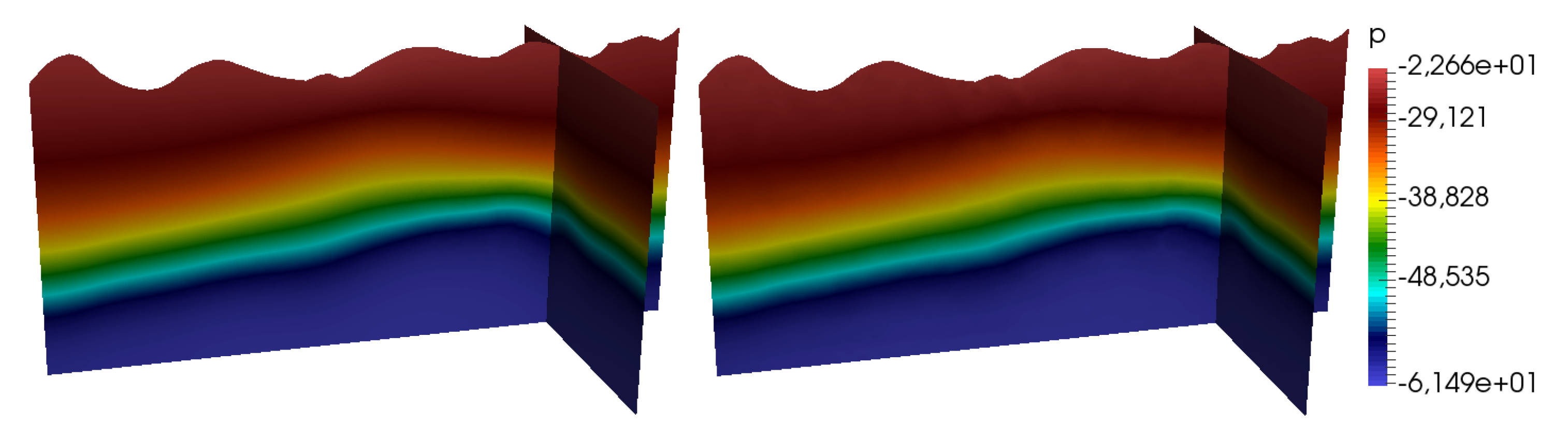
Figure 15.
Numerical results for Test 3.RBC. Solutions p and for the final time. Left: Fine-scale solution = 43,524. Right: Multiscale solution using 32 basis functions = 12,738.
Figure 15.
Numerical results for Test 3.RBC. Solutions p and for the final time. Left: Fine-scale solution = 43,524. Right: Multiscale solution using 32 basis functions = 12,738.
Table 1.
Numerical results for Test 1.DBC. Relative errors (%) for different numbers of multiscale basis functions.
Table 1.
Numerical results for Test 1.DBC. Relative errors (%) for different numbers of multiscale basis functions.
| Number of Multiscale Basis Functions | | | | |
|---|
| 1 | 76 | 10.271 | 11.519 | 15.397 |
| 2 | 142 | 8.679 | 10.183 | 14.026 |
| 4 | 274 | 2.308 | 2.162 | 2.388 |
| 8 | 538 | 1.163 | 0.883 | 0.885 |
| 12 | 802 | 0.779 | 0.542 | 0.509 |
| 16 | 1066 | 0.607 | 0.413 | 0.373 |
| 24 | 1594 | 0.465 | 0.307 | 0.265 |
| 32 | 2122 | 0.375 | 0.247 | 0.208 |
Table 2.
Numerical results for Test 1.NBC. Relative error (%) for different numbers of multiscale basis functions.
Table 2.
Numerical results for Test 1.NBC. Relative error (%) for different numbers of multiscale basis functions.
| Number of Multiscale Basis Functions | | | | |
|---|
| 1 | 76 | 6.474 | 22.111 | 103.246 |
| 2 | 142 | 5.989 | 19.231 | 92.872 |
| 4 | 274 | 1.332 | 1.719 | 3.416 |
| 8 | 538 | 0.442 | 0.561 | 1.119 |
| 12 | 802 | 0.275 | 0.327 | 0.621 |
| 16 | 1066 | 0.189 | 0.229 | 0.428 |
| 24 | 1594 | 0.126 | 0.154 | 0.287 |
| 32 | 2122 | 0.105 | 0.123 | 0.221 |
Table 3.
Numerical results for Test 1.RBC. Relative error (%) for different numbers of multiscale basis functions.
Table 3.
Numerical results for Test 1.RBC. Relative error (%) for different numbers of multiscale basis functions.
| Number of Multiscale Basis Functions | | | | |
|---|
| 1 | 76 | 7.665 | 21.611 | 83.572 |
| 2 | 142 | 7.067 | 18.645 | 63.629 |
| 4 | 274 | 1.384 | 1.691 | 2.834 |
| 8 | 538 | 0.449 | 0.564 | 0.941 |
| 12 | 802 | 0.278 | 0.332 | 0.531 |
| 16 | 1066 | 0.194 | 0.233 | 0.363 |
| 24 | 1594 | 0.131 | 0.155 | 0.242 |
| 32 | 2122 | 0.108 | 0.123 | 0.187 |
Table 4.
Numerical results for Test 2.DBC. Relative error (%) for different numbers of multiscale basis functions.
Table 4.
Numerical results for Test 2.DBC. Relative error (%) for different numbers of multiscale basis functions.
| Number of Multiscale Basis Functions | | | | |
|---|
| 1 | 76 | 11.638 | 13.598 | 18.156 |
| 2 | 142 | 9.896 | 11.671 | 15.968 |
| 4 | 274 | 2.422 | 2.308 | 2.703 |
| 8 | 538 | 1.272 | 0.958 | 1.036 |
| 12 | 802 | 0.911 | 0.666 | 0.701 |
| 16 | 1066 | 0.711 | 0.507 | 0.496 |
| 24 | 1594 | 0.526 | 0.378 | 0.356 |
| 32 | 2122 | 0.432 | 0.306 | 0.277 |
Table 5.
Numerical results for Test 2.NBC. Relative error (%) for different numbers of multiscale basis functions.
Table 5.
Numerical results for Test 2.NBC. Relative error (%) for different numbers of multiscale basis functions.
| Number of Multiscale Basis Functions | | | | |
|---|
| 1 | 76 | 12.599 | 56.362 | 105.404 |
| 2 | 142 | 10.662 | 48.594 | 106.478 |
| 4 | 274 | 2.935 | 8.343 | 34.101 |
| 8 | 538 | 0.883 | 1.886 | 6.951 |
| 12 | 802 | 0.568 | 1.171 | 4.132 |
| 16 | 1066 | 0.383 | 0.724 | 2.328 |
| 24 | 1594 | 0.276 | 0.487 | 1.535 |
| 32 | 2122 | 0.203 | 0.333 | 1.005 |
Table 6.
Numerical results for Test 2.RBC. Relative error (%) for different numbers of multiscale basis functions.
Table 6.
Numerical results for Test 2.RBC. Relative error (%) for different numbers of multiscale basis functions.
| Number of Multiscale Basis Functions | | | | |
|---|
| 1 | 76 | 12.907 | 39.998 | 92.513 |
| 2 | 142 | 10.889 | 32.043 | 91.271 |
| 4 | 274 | 2.607 | 5.064 | 11.835 |
| 8 | 538 | 0.841 | 1.324 | 2.765 |
| 12 | 802 | 0.551 | 0.827 | 1.671 |
| 16 | 1066 | 0.386 | 0.551 | 1.032 |
| 24 | 1594 | 0.279 | 0.381 | 0.704 |
| 32 | 2122 | 0.211 | 0.271 | 0.479 |
Table 7.
Numerical results for Test 3.DBC. Relative error (%) for different numbers of multiscale basis functions.
Table 7.
Numerical results for Test 3.DBC. Relative error (%) for different numbers of multiscale basis functions.
| Number of Multiscale Basis Functions | | | | |
|---|
| 1 | 462 | 9.505 | 10.401 | 12.483 |
| 2 | 858 | 8.074 | 9.198 | 11.376 |
| 4 | 1650 | 4.112 | 4.061 | 5.356 |
| 8 | 3234 | 2.609 | 2.374 | 3.068 |
| 12 | 4818 | 1.411 | 1.253 | 1.556 |
| 16 | 6402 | 0.997 | 0.889 | 0.997 |
| 24 | 9570 | 0.657 | 0.528 | 0.521 |
| 32 | 12,738 | 0.469 | 0.339 | 0.324 |
Table 8.
Numerical results for Test 3.NBC. Relative error (%) for different numbers of multiscale basis functions.
Table 8.
Numerical results for Test 3.NBC. Relative error (%) for different numbers of multiscale basis functions.
| Number of Multiscale Basis Functions | | | | |
|---|
| 1 | 462 | 8.598 | 26.347 | 54.516 |
| 2 | 858 | 7.554 | 24.525 | 52.081 |
| 4 | 1650 | 2.566 | 6.072 | 19.783 |
| 8 | 3234 | 1.292 | 2.594 | 7.792 |
| 12 | 4818 | 0.718 | 1.194 | 3.591 |
| 16 | 6402 | 0.577 | 0.744 | 2.163 |
| 24 | 9570 | 0.379 | 0.421 | 1.118 |
| 32 | 12,738 | 0.259 | 0.271 | 0.646 |
Table 9.
Numerical results for Test 3.RBC. Relative error (%) for different numbers of multiscale basis functions.
Table 9.
Numerical results for Test 3.RBC. Relative error (%) for different numbers of multiscale basis functions.
| Number of Multiscale Basis Functions | | | | |
|---|
| 1 | 462 | 14.344 | 31.851 | 64.631 |
| 2 | 858 | 12.372 | 27.955 | 55.481 |
| 4 | 1650 | 3.834 | 5.904 | 13.551 |
| 8 | 3234 | 1.891 | 2.344 | 4.924 |
| 12 | 4818 | 0.862 | 1.111 | 2.138 |
| 16 | 6402 | 0.583 | 0.738 | 1.342 |
| 24 | 9570 | 0.339 | 0.409 | 0.691 |
| 32 | 12,738 | 0.221 | 0.251 | 0.398 |


