Coordination Supply Chain Management Under Flexible Manufacturing, Stochastic Leadtime Demand, and Mixture of Inventory

Abstract

The necessity of coordination among entities is essential for the success of any supply chain management (SCM). This paper focuses on coordination between two players and cost-sharing in an SCM that considers a vendor and a buyer. For random demand and complex product production, a flexible production system is recommended. The study aims to minimize the total SCM cost under stochastic conditions. In the flexible production systems, the production rate is introduced as the decision variable and the unit production cost is minimum at the obtained optimal value. The setup cost of flexible systems is higher and to control this, a discrete investment function is utilized. The exact information about the probability distribution of lead time demand is not available with known mean and variance. The issue of unknown distribution of lead time demand is solved by considering a distribution-free approach to find the amount of shortages. The game-theoretic approach is employed to obtain closed-form solutions. First, the model is solved under decentralized SCM based on the Stackelberg model, and then solved under centralized SCM. Bargaining is the central theme of any business nowadays among the players of an SCM to make their profit within a centralized and decentralized setup. For this, a cost allocation model for lead time crashing cost based on the Nash bargaining model with the satisfaction level of SCM members is proposed. The cost allocation model under Nash bargaining achieves exciting results in SCM coordination.

1. Introduction

Supply chain management (SCM) depicts the effective management of information, materials, financial flows, and products across the chain, expanding it across supplier, manufacturer, retailer, distributor, and end customer. SCM aims to minimize risks and uncertainties in the chain. It facilitates the flow of raw materials, smooth production, and on-time final product delivery to the end customers [1,2]. The authors consider the problem of coordination in a single buyer single vendor SCM when demand at the buyer’s end is stochastic. In the decentralized decision making, the members of the SCM try to minimize their costs without considering other members’ costs. While in centralized decision making, there is one central planner who optimizes the decision variable to reduce the SCM cost by collecting all the information from all participants of the SCM. Therefore, coordination policies are a crucial factor in reducing the cost of the SCM and bringing savings to the individual SCM participants [3,4].

In the traditional SCM models, the production rate is considered a fixed parameter. However, in many real industrial cases, the production systems are considered as flexible systems [5,6]. The production flexibility implies that the rate of production of a machine or production system can vary quickly [7]. With flexibility in the production system, the vendor can reduce the cost by controlling the inventory. The literature on flexible production systems with variable production rates is limited as compared to other directions, and coordination it needs more consideration. Therefore, the proposed study considers the flexible production system with variable production rates. With the increase in production rate, the tool failure and tool cost may increase, which can cause deterioration in the quality of products. A production process with the robotic assembly system can be the best example of this idea. The increase in the rate of production causes a decrease in robot repeatability [8]. Hence, a certain percentage of production quality is reduced by a higher rate of production. Therefore, it is sensible to accept the production rate as a decision variable instead of the fixed parameter.

In contrast to previously proposed Joint Economic Lot Size (JELS) models, this study aims to assess the performance of the centralized, decentralized, and coordinated inventory strategies in terms of SCM costs or profitability. However, many previous studies on different stochastic inventory or SCM models were mainly normally distributed demand-based continuous review policies for single-vendor single-buyer. In real cases, it is too difficult to find the exact information regarding the probability distribution function of lead time demands. Authors found that existing literature on vendor–buyer inventory coordination policies, especially for controllable lead time, imperfect production systems, stochastic demand with incomplete information, is very limited. In SCM models for vendor and buyer, no study considered the controllable production rate to evaluate the impact on SCM cost minimization. In addition, mostly researches consider setup cost as a fixed parameter but, in developed technological systems, it is reducible with the addition of initial investment. The coordination in proposed SCM focuses on the optimal cost allocation ratio for crashing costs to be shared by the vendor under a stochastic environment. Considering this coordinated SCM, the incentive sharing contracts may work well to achieve extra savings in cost for all participants. In brief, the major research questions to be addressed in this research are:

• Can players’ coordination benefit the SCM to reduce or control total cost when lead time demands are stochastic?
• Does the vendor (manufacturer) get help to reduce production cost and overall cost of the SCM by adopting the variable production rate policy?
• How would the decentralized model established on the Stackelberg approach, the centralized optimization model, and the coordination model perform under the controllable lead time?
• If partial backorders and lost sales costs are permitted, is there a stochastic coordination policy that can come up with a lower cost than the other policies?

The lead time demand is assumed stochastic and production rate is regarded as a decision variable, whether the coordination policy still rewards the single-buyer single-vendor setting is the primary question authors are interested. The expected total system cost measures the overall performance of the stochastic centralized, decentralized, and coordinated SCM policies. This study intends to initiate a stochastic SCM policy that responds better than the traditional stochastic decentralized decision making policy.

1.1. Literature Review

In this section, authors discuss two research directions that are directly related to the work and investigates, (I) Inventory and production models with variable production rate and (II) SCM with vendor–buyer coordination policy. In the second stream, the authors will be focusing on single-buyer single-vendor SCM models.

1.1.1. Inventory and Production Models with Variable Production Rate

Traditional SCM and production models consider the production rate a fixed parameter. However, determining the optimal production rate for a production system has initially begun to get researchers’ attention in recent years. In this research direction, Khouja [9] was the first to introduce production flexibility to expand the basic Economic Production Quantity (EPQ) models by recognizing that the rate of production can be adjusted before the production cycle starts. Their model proposed that the obtained optimal rates may be higher or smaller than the initial rate that keeps the unit costs to the minimum value in volume-flexible production systems. Further, Khouja and Mehrez [10] assumed the impact of the production rate on the quality of the final product. The results of their model suggested that the increase in the production rate induces an evident decay in products’ quality and the obtained optimal production rates are lower than the value that actually keeps unit cost of production to the minimum. In contrast, the optimal rate might be higher than the value that reduces the unit cost, where product quality is not affected by the rate of production.

Moreover, this work [10] was extended in Khouja [11] by suggesting that the production system may move to an out-of-control state randomly and depending on the rate of production. The authors established that integrating production quality in model with the variable production rate results in a smaller lot size and a shorter cycle length. A model was introduced to obtain both the optimal production rate and cycle time by Eiamkanchanalai and Banerjee [12]. The authors introduced the objective function with a desirability term and proved that the optimal rate of production could be smaller or larger than the rate that reduces the production cost. Further, Giri et al. [13] formulated an EPQ model under the deteriorating conditions and the failure rate caused by the stress level of the system or machine increases with the increase in production rate. The work of Giri et al. [13] was extended to the maintenance and stochastic demand [14], unrealizable manufacturing system and inspection sampling size [15], and stochastic machine failures and repair time [16].

Glock [17] developed two-stage production models with equal-sized and unequal-sized batch sizing model and introduced the variable production rate. Production rate is considered within limit $P_{min}$ and $P_{max}$, while $P_{min}$ is considered always greater than D. Glock’s [17] model was extended by himself Glock, [18]) for controlling the inventory in multi-stage production, lot-sizing, and with variable production rate. A vendor–buyer integrated inventory control model with lead time reduction and variable production rate was formulated by Glock [3]. In the model, lead time dependent lot size with stochastic demand was considered. Recently, AlDurgam and Duffuaa [1] utilized the Markov Decision Process by introducing multiple production machines and different quality states. The decision-makers find the optimal maintenance action and the production rate to maximize the manufacturing system’s effectiveness. Sarkar et al. [7] presented a model with joint decision making where a single vendor and multiple buyers are considered. Their model is based on three different production functions on the basis of product quality. They concluded that the increase in production rate might affect product quality. Sarkar and Chung [8] proposed a work-in-process inventory model for flexible production under the investments. They considered the automation based smart production process. Malik and Kim [5] developed a constrained mathematical model for the flexible production system in relation to the optimal production rates and environmental impact. Finally, Dey et al. [19] developed a mathematical model for the work-in-process inventory under the autonomation smart production system. They discussed the single-stage manufacturing under the profit maximization problem.

1.1.2. SCM with Vendor-Buyer Coordination Policy

Integrated inventory models or Joint Economic Lot Size (JELS) models have gained popularity among researchers in recent decades. In traditional SCM, buyers and vendors make efforts for benefits independently to minimize their costs. In contrast, centralized decision-making systems have improved the performance and reduced the cost of the entire SCM. Further, coordinated SCM have been observed improving the performance and effectiveness of the whole SCM in terms of the expected total cost of the system and strategic partnership among participants [20]. Hence, coordinated SCM are becoming socially and economically motivated SCM strategies. The literature on JELS models and coordination contracts has dramatically increased since Goyal’s model (Goyal, 1976). For a comprehensive study of related literature, the readers should look into Glock (2012) [21].

Goyal [22] was the first to propose an integrated (vendor–buyer) inventory model and illustrated the economic advantage of joint decision-making in the supply chain. The assumption of an infinite production rate in Goyal’s model was relaxed, by Banerjee [23], and extended the model to the lot-for-lot policy when the vendor and the buyer coordinate for the consumption and production cycles. In the same way, the model of Banerjee [23] was extended to account for multiple shipments with the identically sized lots that the vendor sends to the buyer by the Lu [24]. Further, the works of Banerjee [23] and Lu [24] was extended by Goyal [25] assuming the geometric increase in the batch size of subsequent batches. Hill [26] generalized Goyal model by considering the optimal shipment policy, which comprises of a combinations of equal- and unequal-sized lot shipments. Many other authors have studied the optimal batch size problems in different inventory models, Huang [27] and Wee and Widyadana [28] are among others.

In the literature, researchers have considered well-established long-run strategic partnerships among SC members, who can cooperate in following a centralized policy and reaching the optimal decisions [29,30]. However, SCM without the central planner may have conflicts over incentives. A conflict of interest occurs in a SC because members may have different and sometimes conflicting objectives. The SC members must work to develop a collaborative plan for successful information sharing, production and inventory planning, and shipment policies. Ye and Xu [31] introduced a cost allocation plan for the vendor–buyer SC to strengthen the strategic partnership between players. They presented a bargaining policy to find a reasonable cost-sharing ratio between the buyer and the vendor. Kunter, [32] formulated a cooperative SC model for the electronics industry with a revenue-and-cost-sharing strategy based on the bargaining model. Heydari, [33] proposed an SCM coordination scheme based on the lead time variation control and reliable shipments. Heydari, [34] analyzed the lead time aggregation phenomena in a two-echelon SC under the stochastic conditions and proposed extra payment strategy for the coordination. Saha and Goyal [2] developed three coordinating policies; (a) wholesale price discount, (b) joint rebate, and (c) cost sharing, for two echelon SCM coordination perspectives. They considered the stock and price dependent demand. Further, Heydari et al. [35] (2016) extended the model to three-echelon SC and presented a reorder point based coordination mechanism for the profitability of SC.

Basiri and Heydari [36] developed coordination model for the green SCM with product substitutions. Authors considered green quality, selling price, and sales efforts for the coordination contracts. Moon et al. [37] studied the coordination and investment decisions in an SCM of fresh agricultural products. They presented three different scenarios, decentralized, revenue sharing with investment costs sharing, incremental quantity discount policy, and compared the results. Malik and Sarkar [38] proposed coordination SCM model for the stochastic-fuzzy demands with two modes of transportation to reduce the leadtime. Daryanto et al. [39] studied the coordination SCM model for deteriorating production with two different inspection policies. They considered carbon emission from storage space and transportation process. Saha et al. [4] studied channel coordination mechanism for three echelon SCM for price and sales efforts sensitive demand. Recently, Xin et al. [40] formulated the coordination SCM for the green products under the fuzzy demands. They proposed three contract policies named two-part tariff, green product cost-sharing, and wholesale price-only.

To solve the stochastic demand problems, researchers generally consider the normal probability distribution to find the expected lead time demand. However, in real-life situations, the exact information about the lead time demands is unavailable and hence difficult to find the probability distribution function. To solve this issue, Gallego and Moon [41] simplified the distribution-free approach proposed by Scarf [42]. Further, Moon and Choi [43] used the distribution-free approach to solve the inventory problems with an unknown probability distribution. Since then, the distribution-free approach has been utilized by numerous researchers to solve the inventory, production, and SCM problems. Tajbakhsh [44] introduced the fill-rate based service level constraint and adopted the distribution-free approach to solving the inventory problem. Moon et al. [45] solved the inventory model considering controllable lead time, demand fill-rate, and unknown distribution function for the stochastic demand. Sarkar et al. [46] proposed a continuous-review inventory model under service level constraint and investments for setup cost reductions and quality improvements. Shin et al. [47] extended the continuous review model with transportation discounts and demand fill-rate. Malik and Sarkar [48] studied the inventory model for a distribution-free approach with controllable lead time, variable setup cost, and backorder price discounts. Further, studies in this direction can be found in Malik and Sarkar [49], Moon et al. [50], and Guchhait et al. [51].

The literature discussed has established that advancing from an assumption where one of the SCM members completely controls the SCM to a setting in which a centrally coordinated solution is attained for the SCM, enhances the performance of the entire SCM. However, a coordinated scheme may put participants of the SCM at a disadvantage in terms of personal cost. To convince all SCM members to distribute the cooperation gain or incentive among all the parties involved, a coordination scheme might be used. The coordination mechanisms that may be used in an SCM includes the information-sharing mechanisms, the design of contracts, strategic alliances, or risk sharing such as consignment stock (CS) or vendor managed inventory (VMI). For the comprehensive literature review of the coordination supply chain, the interested readers are referred to Sarmah et al. [52] and Kanda and Deshmukh [53]. Recently, many researchers presented different coordination SC models, i.e., revenue sharing, cost-sharing, quantity discounts, and cooperative advertising, to enhance the performance of the SC in terms of profitability and customer service. However, researchers did not consider the variable production rate and the stochastic demands with unknown distribution function for the flexible production systems with the imperfect production process.

2. Problem Definition, Mathematical Notation, and Basic Assumptions

In the section, authors present research problem, basic model assumption. The list of notation used for the formulation of model is given at the end of this article.

2.1. Problem Definition

This study is an attempt develop a single-vendor and single-buyer SCM model when the lead time demand is stochastic but the exact information about probability distribution is unknown. In this proposed model, the vendor manufactures an integer multiple of the buyer’s order quantity (Q) in single setup and delivers the products to the buyer in multiple shipments. The production rate has always a direct impact on the performance of manufacturing system. Therefore, the production is considered as decision variable and unit production cost varies with the variation in production rate. The specific ratio ($\eta$) of shortage amount is backordered at a price and fulfills the demand at the arrival of new replenishment. While the rest of the shortage amount (1–$\eta$) is a lost sales per cycle. This is for the first time in literature that the coordination model between vendor and buyer is being proposed when the production rate and setup cost are taken decision variable along with the unknown distribution problem of lead time demand. This Section presents a mathematical model for the described problem and solved it with three strategies: (1) decentralized decision making established on the Stackelberg model, (2) the centralized decision making model, and (3) asymmetric Nash bargaining model for coordination.

2.2. Assumptions

1.

The coordination SCM model with buyer-vendor setting is considered. A single type of product is produced and offered to the buyer.

2.

The buyer reviews the inventory level continuously. The moment inventory level hits the reorder point, the buyer instantly places an order of quantity Q.

3.

Single-setup-multi-delivery policy is adopted, which means vendor manufacturers quantity $nQ$ in single production setup, with a finite production rate, after receiving the buyer’s order of quantity Q. After every $\frac{Q}{D}$ time units as an average, a shipment of size Q is transferred from vendor to the buyer.

4.

The production rate is assumed as an adjustable quantity which varies between the range $P_{min}$ and $P_{max}$, when the $P_{min}>D$. The unit production cost is direct function of the production rate P and calculated as $C_v=C_{mat}+\frac{C_i}{P}+\gamma P$.

5.

Produced products are inspected multiple times before dispatch and defective products are shifted to the reworking station. An inspection cost belongs entirely to the vendor’s cost component. Reworked products are considered as perfect as new and shipped to the buyer immediately without holding those products (see for reference, [54]).

6.

Shortages are permitted at the buyer’s end and a described ratio of $\eta$ of shortages is backordered at a price $\pi$ per unit backordered.

7.

To control the setup cost, extra discrete investments are required (see for reference, [55]). Thus, the model considers an investment function $S\left(J_i\right)=S_0{e}^{-r{J}_i}$ which is discrete in nature. Here, S is setup cost per production cycle and strictly decreasing function of J, r is a predefined parameter and estimated from the data, and $J_i$ is the investment for vendor, $i=0,1,\dots ,n$ and $J_0=0$.

8.

The lead time is controllable with additional crashing cost $C\left(L\right)$. The lead time crashing cost is calculated by $C\left(L\right)=c_i(L_{i-1}-L)+{\sum }_{j=1}^{i-1}{c}_j(b_j-a_j)$. The crashing cost is owed altogether to the buyer’s cost component in assumed centralized and decentralized SCM. In coordination model, the ratio $\theta$ of the crashing cost is paid by the vendor and rest of part is burdened by the buyer which is $(1-\theta )$. This $\theta$ basically depends on the bargaining power of the player of the integrated model (see for reference [56]).

3. Mathematical Model

There are two SCM players in the proposed study, one is buyer and the other is vendor. First, the buyer’s mathematical model is discussed and then, the vendor’s mathematical model is developed, respectively.

3.1. Buyer’s Mathematical Model

In this section, the buyer’s cost and total cost are calculated with established notation and assumptions, as follows

3.1.1. Ordering Cost ($OC$)

The buyer adopts continuous review inventory managing policy and places an order as the inventory level drops to the reorder point. It costs some funds every time the buyer places an order. The order cost for each order is A and the cycle length for the buyer is $Q/D$. Hence, the ordering cost is calculated as

$$\begin{array}{c}\hfill OC=\frac{A_{b}D}{Q}.\end{array}$$

3.1.2. Maintenance Cost ($MC$)

This model considers the maintenance cost for the buyer explicitly. Buyer’s maintenance cost is counted once per cycle.

$$\begin{array}{ccc}\hfill MC& \hfill =\hfill & \frac{\mathrm{Buyer}’\mathrm{s}\mathrm{maintenance}\cos \mathrm{t}}{\mathrm{Cycle}\mathrm{time}}\hfill \\ & \hfill =\hfill & \frac{C_{M}D}{Q}.\hfill \end{array}$$

3.1.3. Inventory Holding Cost

The overall inventory level prior to the replenishment is $R-DL$ and immediately after receiving the quantity Q makes it $Q+R-DL$. Thus, the calculated average inventory for the buyer in this model is

$$\begin{array}{c}\hfill I_{avg}=\left(\frac{Q}{2}+R-DL\right).\end{array}$$

The lead time demand is random in nature and $k\sigma \sqrt{L}=R-DL$. Accordingly, the average inventory can be obtained as

$$\begin{array}{c}\hfill I_{avg}=\left(\frac{Q}{2}+k\sigma \sqrt{L}\right).\end{array}$$

This model considers the lead time demand is stochastic with only limited information i.e., unknown distribution function. Therefore, the expected shortages are calculated based on the minmax distribution-free approach introduced by [42] and further [41] explained it in details and simplified if for the practical use. By using minmax distribution free approach, one can obtain $E{(X-R)}^{+}$ for the worst distribution function F.

Proposition 1.

$$\begin{array}{ccc}\hfill E{(X-R)}^{+}& \le & \frac{\sqrt{{\sigma }^{2}L+{(R-DL)}^2}-(R-DL)}{2}.\hfill \end{array}$$

(1)

Here, the upper bound of the equation is tight. The inequality in Equation (1) applies for any distribution of the demand X during lead time and $k\sigma \sqrt{L}=R-DL$. The above inequality can be written as

$$\begin{array}{ccc}\hfill E{(X-R)}^{+}& \le & \frac{\sigma \sqrt{L}(\sqrt{1+k^2}-k))}{2},\hfill \end{array}$$

(2)

the average inventory can be written as

$$\begin{array}{ccc}\hfill I_{avg}& \hfill =\hfill & \left(\frac{Q}{2}+E{(X-R)}^{+}\right)\hfill \\ \hfill \hfill & \hfill =\hfill & \left(\frac{Q}{2}+\frac{1}{2}\sigma \sqrt{L}(\sqrt{1+k^2}-k))\right).\hfill \end{array}$$

3.1.4. Shortages Cost ($SC$)

As mentioned earlier, the lead time demand is stochastic without specific probability distribution function. The lead time demand has a cdf $\mathit{F}$ with the $DL$ as mean and $\sigma \sqrt{L}$ the standard deviation. The shortages happens when the $X>R$, and the expected amount is $E{(X-R)}^{+}\le \frac{1}{2}\sigma \sqrt{L}(\sqrt{1+k^2}-k))$ at the end of the cycle. The backorder cost per unit is $\pi$ and total backordering cost is

$$\begin{array}{ccc}\hfill BC& \hfill =\hfill & \frac{\pi DE{(X-R)}^{+}}{Q}\hfill \\ \hfill \hfill & =& \frac{\pi D\sigma \sqrt{L}(\sqrt{1+k^2}-k)}{2Q}.\hfill \end{array}$$

The expected lost sales are

$$\begin{array}{ccc}\hfill LC& =& \frac{\delta (1-\eta )DE{(X-R)}^{+}}{Q}\hfill \\ & =& \frac{\delta (1-\eta )D\sigma \sqrt{L}(\sqrt{1+k^2}-k)}{2Q}.\hfill \end{array}$$

Hence, the total shortages cost can be calculated as

$$\begin{array}{ccc}\hfill SC& =& \frac{(\pi +\delta (1-\eta ))DE{(X-R)}^{+}}{Q}\hfill \\ & =& \frac{(\pi +\delta (1-\eta ))D\sigma \sqrt{L}(\sqrt{1+k^2}-k)}{2Q}.\hfill \end{array}$$

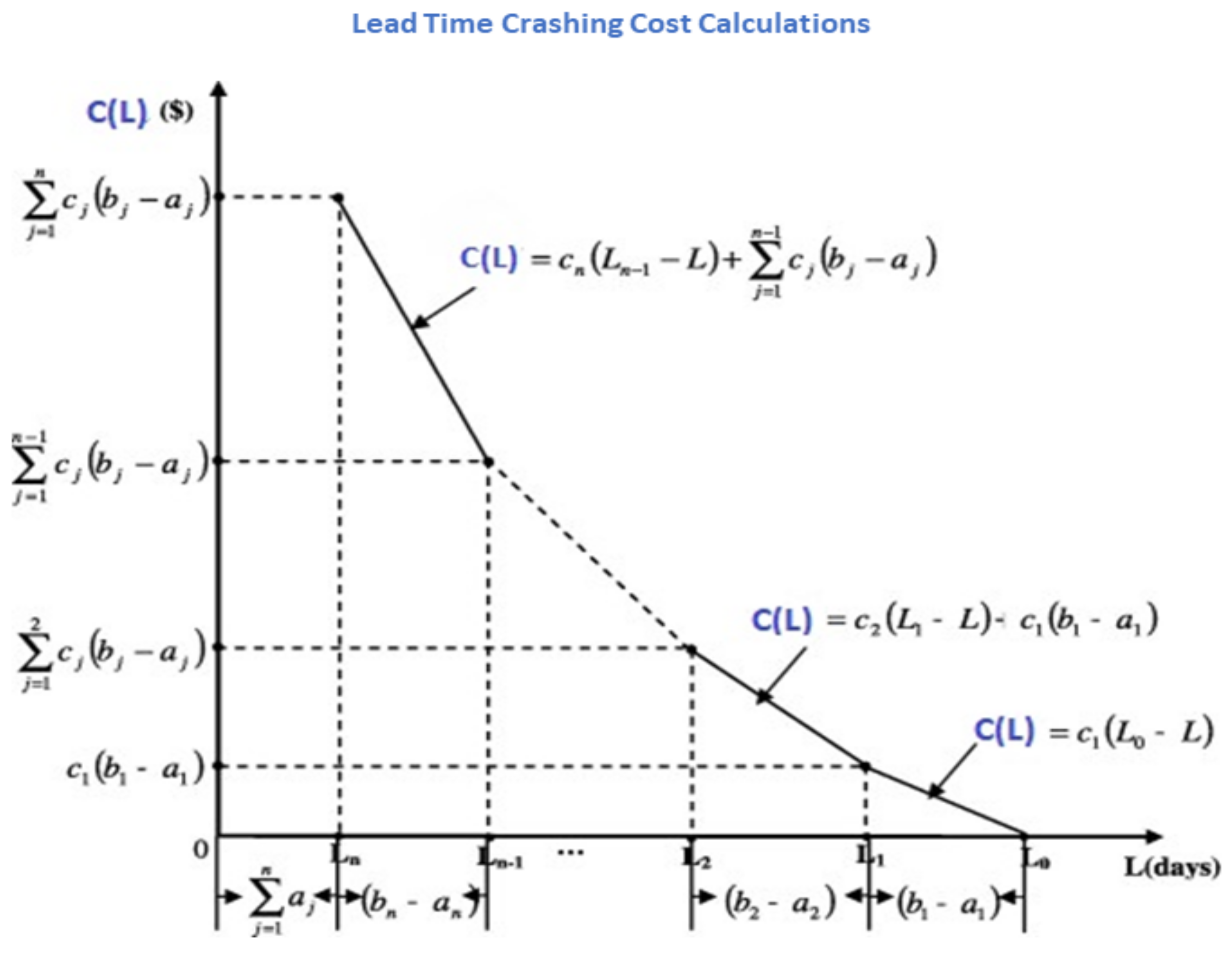
3.1.5. Lead Time Crashing Cost ($LTC$)

The lead time crashing cost per cycle can be calculated as follows

$$\begin{array}{ccc}\hfill LTC\hfill & =& \frac{\mathrm{lead}\mathrm{time}\mathrm{crashing}\cos \mathrm{t}}{\mathrm{cycle}\mathrm{time}}\hfill \\ & =& \frac{C\left(L\right)D}{Q}.\hfill \end{array}$$

The crashing cost $C\left(L\right)$ for the given lead time ′$L\in [L_i,L_{i-1}]$’ is

$$\begin{array}{c}\hfill C\left(L\right)=c_i(L_{i-1}-L)+\sum _{j=1}^{i-1}{c}_j(b_j-a_j).\end{array}$$

The lead time is composed of n independent small components. Each component has a fixed minimum duration ($a_i$) and the normal duration $b_i$. Each component crashing cost per unit time is $c_i$. Moreover, for convenience, arrange $c_i$ such that $c_1\le c_2\le \dots \le c_n$. It is assumed $L_0={\sum }_{j=1}^n{b}_j$ and $L_i$ is lead time duration with components $1,2,\dots i$ (see Figure 1).

3.1.6. Buyer’s Expected Total Cost ($T{C}_b$)

Buyer’s expected total cost is calculated as follows:

$$\begin{array}{ccc}\hfill TEA{C}_b& =& \mathrm{Ordering}\cos \mathrm{t}+\mathrm{Maintenance}\cos \mathrm{t}+\mathrm{Inventory}\mathrm{holding}\cos \mathrm{t}+\mathrm{Shortages}\cos \mathrm{t}\hfill \\ & +& \mathrm{Lead}\mathrm{time}\mathrm{crashing}\cos \mathrm{t}\hfill \end{array}$$

Hence, the buyer’s expected total cost is

$$\begin{array}{ccc}\hfill T{C}_b(Q,L,k)& =& \frac{A_{b}D}{Q}+\frac{C_{M}D}{Q}+h_b\left[\frac{Q}{2}+k\sigma \sqrt{L}+(1-\eta )\frac{1}{2}\sigma \sqrt{L}(\sqrt{(1+k^2)}-k)\right]\hfill \\ & +& (\pi +\delta (1-\eta ))\frac{1}{2}\sigma \sqrt{L}(\sqrt{(1+k^2)}-k)\frac{D}{Q}+\frac{DC\left(L\right)}{Q}.\hfill \end{array}$$

(3)

3.2. Vendor’s Mathematical Model

First, authors calculate the setup cost, investment function for the setup cost reduction, the unit production cost, inventory holding cost, inspection cost, and reworking cost for vendor are calculated. Then, all these mentioned costs are added to obtain the annual expected cost for vendor.

3.2.1. Setup Cost

The vendor has a fixed initial setup cost of $S_0$. The vendor is interested to invest the amount of J for setup improvement to reduce the setup cost (S) for each setup. The number of cycles per year are $\frac{D}{nQ}$. Therefore, the vendor’s setup cost per manufacturing setup can be expressed as:

$$\begin{array}{c}\hfill \mathrm{Setup}\cos \mathrm{t}=\frac{DS\left(J_i\right)}{nQ};\mathrm{where},S\left(J_i\right)=S_0{e}^{-r{J}_i}.\end{array}$$

where r is the known parameter and calculated by the given historical data, and J is the discrete investments to attain setup cost S per setup.

3.2.2. Investment for Setup Cost Reduction

To reduce and control the setup cost, the model considers an additional discrete investment J (see for instance [55]). This is an initial investment. Therefore, to calculate the investment per cycle it is divided by the cycle length $\frac{nQ}{D}$ for the vendor.

$$\begin{array}{c}\hfill \mathrm{Investment}\mathrm{for}\mathrm{setup}\cos \mathrm{t}\mathrm{reduction}=\frac{JD}{nQ}.\end{array}$$

3.2.3. Unit Production Cost

Unit production cost can be considered as

$$\begin{array}{c}\hfill C_v=C_{mat}+\frac{C_i}{P}+\gamma P.\end{array}$$

where P is the production rate, $C_{mat}$ is the raw materials cost per unit produced, $C_i$ is the fixed cost i.e., labor and energy cost, and $\gamma$ denotes the tool and die cost per unit item see for instance [13]. Here, the last term is directly proportional to the production rate P and the second term is inversely proportional to production rate P. Total production cost can be calculated as

$$\mathrm{Production}\mathrm{cost}=C_{v}D.$$

3.2.4. Inventory Holding Cost

The average inventory for the vendor in the this model is

$$\begin{array}{ccc}\hfill I_{avg}& =& \frac{Q}{2}\left[n\left(1-\frac{D}{(1-\varphi )P}\right)-1+\frac{2D}{(1-\varphi )P}\right].\hfill \end{array}$$

To calculate the inventory holding cost for vendor, average inventory is multiplied by the unit holding cost rate of the vendor $h_v$.

$$\begin{array}{c}\hfill \mathrm{Inventory}\mathrm{holding}\cos \mathrm{t}=h_v\frac{Q}{2}\left[n\left(1-\frac{D}{(1-\varphi )P}\right)-1+\frac{2D}{(1-\varphi )P}\right].\end{array}$$

3.2.5. Inspection Cost

This model considers three inspection costs for three inspection steps, variable inspection cost $C_{i0}$ for each shipment, unit inspection cost $C_{ivv}$ for each unit, and fixed inspection cost $C_{ivf}$ for each production lot. All the produced products are inspected and defective products are directly sent to the reworking station. Hence, the total inspection/screening cost per cycle is given as

$$\begin{array}{c}\hfill \mathrm{Inspection}\cos \mathrm{t}=\frac{D}{Q}{C}_{i0}+D{C}_{ivv}+\frac{D}{nQ}{C}_{ivf}.\end{array}$$

3.2.6. Rework Cost

During the production process, a certain percentage of production is imperfect or defective and it is reworked at a cost immediately. Thus, the rework cost is as follows:

$$\begin{array}{c}\hfill \mathrm{Rework}\cos \mathrm{t}=\frac{\varphi P{C}_r}{T}=\frac{C_{r}D\varphi P}{nQ},\mathrm{where}T=\frac{nQ}{D}.\end{array}$$

Hence, the vendors annual expected total cost can be represented as

$$\begin{array}{ccc}\hfill T{C}_v& =& \mathrm{Setup}\cos \mathrm{t}+\mathrm{Investment}\mathrm{for}\mathrm{setup}\cos \mathrm{t}\mathrm{reduction}+\mathrm{Production}\cos \mathrm{t}+\mathrm{Inspection}\cos \mathrm{t}\hfill \\ & +& \mathrm{Holding}\cos \mathrm{t}+\mathrm{Reworking}\cos \mathrm{t}\hfill \end{array}$$

$$\begin{array}{ccc}\hfill T{C}_v(P,J,n)& =& \frac{S_0{e}^{-r{J}_i}D}{nQ}+\frac{JD}{nQ}+C_{v}D+\left(\frac{D}{Q}{C}_{i0}+D{C}_{ivv}+\frac{D}{nQ}{C}_{ivf}\right)\hfill \\ & +& \frac{h_{v}Q}{2}\left[n\left(1-\frac{D}{(1-\varphi )P}\right)-1+\frac{2D}{(1-\varphi )P}\right]+\frac{C_{r}D\varphi P}{nQ}.\hfill \end{array}$$

(4)

4. Solution Methodology

This study considers two different cases to discuss the decision making of vendor and buyer. The two decision making are (1) decision making without any coordination (generally referred to as decentralized decision) and (2) the classical single decision making system (which generally is referred to as centralized decision making).

4.1. Decentralized Mathematical Model

Since vendor and buyer are two different economic entities, therefore, under the decentralized model they do not cooperate in decision making. Hence, they both will try to make such optimal decisions which benefit them more. First, the buyer will decide the order quantity (Q), lead time (L), and inventory safety factory (k) such that his annual cost is minimum. Then, the vendor will decide his optimal values by considering the buyer’s optimal values as an input for the production rate P, investment for setup cost reduction (J), and the number of shipments per cycle (n). The Stackelberg model between the buyer and the vendor is given as follows:

$$\begin{array}{ccc}\hfill T{C}_v(P,J,n,\varphi )& =& \frac{JD}{nQ}+\frac{S_0{e}^{-r{J}_i}D}{nQ}+C_{v}D+\left(\frac{D}{Q}{C}_{i0}+D{C}_{ivv}+\frac{D}{nQ}{C}_{ivf}\right)\hfill \\ & +& \frac{h_{v}Q}{2}\left[n\left(1-\frac{D}{(1-\varphi )P}\right)-1+\frac{2D}{(1-\varphi )P}\right]+\frac{C_{r}D\varphi P}{nQ}.\hfill \end{array}$$

(5)

$$\begin{array}{ccc}\hfill T{C}_b(Q,L,k)& =& \frac{A_{b}D}{Q}+\frac{C_{M}D}{Q}+h_b\left[\frac{Q}{2}+k\sigma \sqrt{L}+(1-\eta )\frac{1}{2}\sigma \sqrt{L}(\sqrt{(1+k^2)}-k)\right]\hfill \\ & +& (\pi +\delta (1-\eta ))\frac{1}{2}\sigma \sqrt{L}(\sqrt{(1+k^2)}-k)\frac{D}{Q}+\frac{DC\left(L\right)}{Q}.\hfill \end{array}$$

(6)

To minimize the annual cost for buyer, the analytical method is applied and partial derivative with respect to (w.r.t) order quantity Q, lead time L, and safety factory k are calculated as follows

$$\begin{array}{ccc}\hfill \frac{\partial T{C}_b(Q,L,k)}{\partial Q}& =& -\frac{A_{b}D}{Q^2}-\frac{C_{M}D}{Q^2}+\frac{h_b}{2}-\frac{D(\pi +\delta (1-\eta ))\sigma \sqrt{L}(\sqrt{(1+k^2)}-k)}{2Q^2}\hfill \\ & -& \frac{DC\left(L\right)}{Q^2}.\hfill \\ \hfill \frac{\partial T{C}_b(Q,L,k)}{\partial L}& =& h_b\left[\frac{k\sigma }{2\sqrt{L}}+\frac{(1-\eta )\sigma (\sqrt{(1+k^2)}-k)}{4\sqrt{L}}\right]\hfill \\ & +& \frac{(\pi +\delta (1-\eta ))D\sigma (\sqrt{(1+k^2)}-k)}{4Q\sqrt{L}}-\frac{D{c}_i}{Q}.\hfill \\ \hfill \frac{\partial T{C}_b(Q,L,k)}{\partial k}& =& h_b\left[\sigma \sqrt{L}+\frac{1}{2}(1-\eta )\sigma \sqrt{L}\left(\frac{k}{\sqrt{(1+k^2)}}-1\right)\right]\hfill \\ & +& (\pi +\delta (1-\eta ))\frac{1}{2}\sigma \sqrt{L}\left(\frac{k}{\sqrt{(1+k^2)}}-1\right)\frac{D}{Q}.\hfill \end{array}$$

To check the second order conditions or the convexity of the $T{C}_b(Q,L,k)$, we calculate the second order partial derivatives w.r.t decision variable for buyer $(Q,L,k)$.

$$\begin{array}{ccc}\hfill \frac{{\partial }^{2}T{C}_b(Q,L,k)}{\partial Q^2}& =& \frac{2A_{b}D}{Q^3}+\frac{2C_{M}D}{Q^3}+\frac{D(\pi +\delta (1-\eta ))\sigma \sqrt{L}(\sqrt{(1+k^2)}-k)}{Q^3}\hfill \\ & +& \frac{2DC\left(L\right)}{Q^3}\ge 0.\hfill \\ \hfill \frac{{\partial }^{2}T{C}_b(Q,L,k)}{\partial L^2}& =& -\frac{h_{b}k\sigma }{4\sqrt[3]{L}}-\left(\frac{(1-\eta )h_b}{8\sqrt[3]{L}}+\frac{(\pi +\delta (1-\eta \left)\right)D}{8Q\sqrt[3]{L}}\right)\sigma (\sqrt{(1+k^2)}-k)\le 0.\hfill \\ \hfill \frac{{\partial }^{2}T{C}_b(Q,L,k)}{\partial k^2}& =& \sigma \sqrt{L}\left(\frac{(1-\eta )h_b}{2}+\frac{(\pi +\delta (1-\eta \left)\right)D}{2Q}\right)(\frac{1}{\sqrt{(1+k^2)}}\hfill \\ & -& \frac{k^2}{\sqrt[3]{(1+k^2)}})\ge 0.\hfill \\ \hfill \frac{{\partial }^{2}T{C}_b(Q,L,k)}{\partial k\partial Q}& =& \frac{{\partial }^{2}T{C}_b(Q,L,k)}{\partial Q\partial k}=-(\pi +\delta (1-\eta ))\frac{1}{2}\sigma \sqrt{L}\left(\frac{k}{\sqrt{(1+k^2)}}-1\right)\frac{D}{Q^2}.\hfill \end{array}$$

Now, one can calculate the Hessian matrix $\left(H\right)$ of the proposed model to prove the optimality of the buyer’s cost function.

$$H=\left[\begin{array}{cc}\frac{{\partial }^{2}T{C}_b(Q,L,k)}{\partial Q^2}& \frac{{\partial }^{2}T{C}_b(Q,L,k)}{\partial Q\partial k}\\ \frac{{\partial }^{2}T{C}_b(Q,L,k)}{\partial k\partial Q}& \frac{{\partial }^{2}T{C}_b(Q,L,k)}{\partial k^2}\end{array}\right]$$

(7)

The first principal minor is calculated as

$$\begin{array}{ccc}\hfill \det .\left(H_{11}\right)& =& \det .\left(\frac{{\partial }^{2}T{C}_b(Q,L,k)}{\partial Q^2}\right)\hfill \\ & =& \frac{2A_{b}D}{Q^3}+\frac{2C_{M}D}{Q^3}+\frac{D(\pi +\delta (1-\eta ))\sigma \sqrt{L}(\sqrt{(1+k^2)}-k)}{Q^3}+\frac{2DC\left(L\right)}{Q^3}\ge 0.\hfill \end{array}$$

The second principal minor is calculated as

$$\begin{array}{c}\hfill \det .\left(H_{22}\right)=\left(\begin{array}{cc}\frac{{\partial }^{2}T{C}_b(Q,L,k)}{\partial Q^2}& \frac{{\partial }^{2}T{C}_b(Q,L,k)}{\partial Q\partial k}\\ \frac{{\partial }^{2}T{C}_b(Q,L,k)}{\partial k\partial Q}& \frac{{\partial }^{2}T{C}_b(Q,L,k)}{\partial k^2}\end{array}\right)\end{array}$$

$$\begin{array}{cc}=& \frac{{\partial }^{2}T{C}_b(Q,L,k)}{\partial Q^2}\times \frac{{\partial }^{2}T{C}_b(Q,L,k)}{\partial k^2}-\frac{{\partial }^{2}T{C}_b(Q,L,k)}{\partial k\partial Q}\times \frac{{\partial }^{2}T{C}_b(Q,L,k)}{\partial Q\partial k}\hfill \\ =& \left[\frac{2A_{b}D}{Q^3}+\frac{2C_{M}D}{Q^3}+\frac{D(\pi +\delta (1-\eta ))\sigma \sqrt{L}(\sqrt{(1+k^2)}-k)}{Q^3}+\frac{2DC\left(L\right)}{Q^3}\right]\hfill \\ \times & \sigma \sqrt{L}\left(\frac{(1-\eta )h_b}{2}+\frac{(\pi +\delta (1-\eta \left)\right)D}{2Q}\right)\left(\frac{1}{\sqrt{(1+k^2)}}-\frac{k^2}{\sqrt[3]{(1+k^2)}}\right)\hfill \\ -& {\left[-(\pi +\delta (1-\eta ))\frac{1}{2}\sigma \sqrt{L}\left(\frac{k}{\sqrt{(1+k^2)}}-1\right)\frac{D}{Q^2}\right]}^2\hfill \\ =& \left[\frac{2A_{b}D}{Q^3}+\frac{2C_{M}D}{Q^3}+\frac{2DC\left(L\right)}{Q^3}\right]\times \sigma \sqrt{L}\left(\frac{(1-\eta )h_b}{2}+\frac{(\pi +\delta (1-\eta \left)\right)D}{2Q}\right)(\frac{1}{\sqrt{(1+k^2)}}\hfill \\ -& \frac{k^2}{\sqrt[3]{(1+k^2)}})+\sigma \sqrt{L}\left(\frac{(1-\eta )h_b}{2}\right)\left[\frac{D(\pi +\delta (1-\eta ))\sigma \sqrt{L}(\sqrt{(1+k^2)}-k)}{Q^3}\right]\hfill \\ +& \frac{D^2{(\pi +\delta (1-\eta ))}^2{\sigma }^{2}L}{2Q^4}\times \left(1-\frac{k}{\sqrt{(1+k^2)}}-\frac{k^2}{(1+k^2)}+\frac{k^3}{\sqrt[3]{(1+k^2)}}\right)\hfill \\ -& \left[\frac{D^2{(\pi +\delta (1-\eta ))}^2{\sigma }^{2}L}{4Q^4}\left(\frac{k^2}{(1+k^2)}-\frac{2k}{\sqrt{(1+k^2)}}+1\right)\right]\hfill \end{array}$$

$$\begin{array}{cc}=& \left[\frac{2A_{b}D}{Q^3}+\frac{2C_{M}D}{Q^3}+\frac{2DC\left(L\right)}{Q^3}\right]\times \sigma \sqrt{L}\left(\frac{(1-\eta )h_b}{2}+\frac{(\pi +\delta (1-\eta \left)\right)D}{2Q}\right)(\frac{1}{\sqrt{(1+k^2)}}\hfill \\ -& \frac{k^2}{\sqrt[3]{(1+k^2)}})+\sigma \sqrt{L}\left(\frac{(1-\eta )h_b}{2}\right)\left[\frac{D(\pi +\delta (1-\eta ))\sigma \sqrt{L}(\sqrt{(1+k^2)}-k)}{Q^3}\right]\hfill \\ +& \frac{D^2{(\pi +\delta (1-\eta ))}^2{\sigma }^{2}L}{2Q^4}\times [\left(1-\frac{k}{\sqrt{(1+k^2)}}-\frac{k^2}{(1+k^2)}+\frac{k^3}{\sqrt[3]{(1+k^2)}}\right)-(\frac{k^2}{2(1+k^2)}\hfill \\ -& \frac{k}{\sqrt{(1+k^2)}}+\frac{1}{2}\left)\right]\hfill \end{array}$$

The 2nd principal minor is positive definite for all the values of k at which

$$\begin{array}{c}\hfill \left(1-\frac{k}{\sqrt{(1+k^2)}}-\frac{k^2}{(1+k^2)}+\frac{k^3}{\sqrt[3]{(1+k^2)}}\right)\ge \left(\frac{k^2}{2(1+k^2)}-\frac{k}{\sqrt{(1+k^2)}}+\frac{1}{2}\right)\end{array}$$

(8)

Hence, from the above Hessian matrix $\left(H\right)$ and second order partial derivatives one can see the annual cost for buyer $T{C}_b(Q,L,k)$ function is convex w.r.t order quantity and inventory safety factor. While, the annual cost for buyer $T{C}_b(Q,L,k)$ is concave for lead time because the second order partial derivative w.r.t lead time L is negative. If one considers the values of Q and k as constant, then, the minimum annual cost for buyer can be obtained at the end points of the given $Lϵ[L_i,Li-1]$ (see for reference [30]). One can attain the optimal order quantity and safety factory for the buyer by equating $\frac{\partial T{C}_b(Q,L,k)}{\partial Q}=0$ and $\frac{\partial T{C}_b(Q,L,k)}{\partial k}=0$ and represented as $Q^{*}$ and $k^{*}$.

$$\begin{array}{ccc}\hfill Q^{*}& =& \sqrt{\frac{2D\left[A_b+C_M+C\left(L\right)+\frac{(\pi +\delta (1-\eta )\sigma \sqrt{L}(\sqrt{1+k^2}-k)}{2}\right]}{h_b}}.\hfill \end{array}$$

(9)

$$\begin{array}{ccc}\hfill \frac{k^{*}}{\sqrt{(1+{k^{*}}^2)}}& =& 1-\frac{2Q{h}_b}{(1-\eta )Q{h}_b+(\pi +\delta (1-\eta ))D}.\hfill \end{array}$$

(10)

The vendor will decide his optimal values by taking the buyer’s optimal decision $(Q^{*},L^{*},k^{*})$ as inputs.

$$\begin{array}{ccc}\hfill \frac{\partial T{C}_v(P,J,n,\varphi )}{\partial P}& =& -\frac{C_{i}D}{P^2}+\gamma D-\frac{h_{v}Q(2-n)D}{2(1-\varphi )P^2}+\frac{C_{r}D\varphi }{nQ}.\hfill \\ \hfill \frac{\partial T{C}_v(P,J,n,\varphi )}{\partial J}& =& \frac{D}{nQ}-\frac{r{S}_0{e}^{-Jr}log\left(e\right)D}{nQ}.\hfill \\ \hfill \frac{\partial T{C}_v(P,J,n,\varphi )}{\partial n}& =& \frac{h_{v}Q}{2}\left(1-\frac{D}{(1-\varphi )P}\right)-\frac{JD}{n^{2}Q}-\frac{S_0{e}^{-r{J}_i}D}{n^{2}Q}-\frac{C_{ivf}D}{n^{2}Q}-\frac{C_{r}DP\varphi }{n^{2}Q}.\hfill \\ \hfill \frac{{\partial }^{2}T{C}_v(P,J,n,\varphi )}{\partial P^2}& =& \frac{2C_{i}D}{P^3}+\frac{h_{v}Q(2-n)D}{(1-\varphi )P^3}.\hfill \\ \hfill \frac{{\partial }^{2}T{C}_v(P,J,n,\varphi )}{\partial J^2}& =& \frac{D{r}^{2}S{e}^{-Jr}{log}^2\left(e\right)}{nQ}>0.\hfill \\ \hfill \frac{{\partial }^{2}T{C}_v(P,J,n,\varphi )}{\partial n^2}& =& \left(\frac{2JD}{n^{3}Q}+\frac{2S_0{e}^{-r{J}_i}}{n^{3}Q}+\frac{2C_{ivf}}{n^{3}Q}+\frac{2C_{r}P\varphi }{n^{3}Q}\right)D>0.\hfill \end{array}$$

The annual cost for the vendor $T{C}_v(P,J,n)$ is convex with respect to P, J, and n for fixed Q, k, and $Lϵ[L_i,Li-1]$. Hence, one can obtain the optimal value for production rate $P^{*}$ by equating $\frac{\partial T{C}_v(P,J,n)}{\partial P}=0$.

$$\begin{array}{c}\hfill P^{*}=\sqrt{\frac{nQ[2(1-\varphi )C_i+h_{v}Q(2-n)]}{2(nQ\gamma +C_r\varphi )(1-\varphi )}}.\end{array}$$

(11)

The optimal number of lots $n^{*}$ are decided by the vendor by estimating the buyer’s $Q^{*}$ optimal order quantity. $T{C}_b$ is convex for n with fixed value of parameters, and $L\in [L_i,Li-1]$, hence, the vendor’s optimal $n=n^{*}$ value is obtained, only while

$$\begin{array}{c}\hfill \left\{\begin{array}{c}T{C}_v\left(n^{*}\right)\le T{C}_v(n^{*}+1),\hfill \\ T{C}_v\left(n^{*}\right)\le T{C}_v(n^{*}-1).\hfill \end{array}\right.\end{array}$$

(12)

From the above equation, one can get that $n^{*}$ is the integer value which satisfies the relation

$$\begin{array}{c}\hfill n^{*}(n^{*}-1)\le \frac{2D\left[J+C_{ivf}+S_0{e}^{-r{J}_i}+C_{r}P\varphi \right]}{h_v{\left(Q^{*}\right)}^2\left(1-\frac{D}{(1-\varphi )P^{*}}\right)}\le n^{*}(n^{*}+1).\end{array}$$

(13)

To calculate the optimal values of the decision variables for centralized decision making, authors propose the Algorithm 4.1.

Algorithm 4.1
Step 1:	Assign $n=1$;
Step 2:	For each individual $L_i$ and $i=1,2,\dots z:$ follow 2-i to 2-iv.
Step 2-i:	Using Equation (17) evaluate $Q_i$
Step 2-iii:	Utilize $Q_i$ and Equation (18), to determine the value of $k_i$
Step 2-iv:	Repeat 2-i to 2-iv until no further changes occur in the values of $Q_{i1}$ and ${\omega }_i$, denote these
	values by ($Q_i^{*}$ and $r_i^{*}$).
Step 3:	For each pair values of $(Q_i,L_i,k_i)$, estimate the expected annual cost $T{C}_b(Q_i,L_i,k_i)$ for the
	buyer.
Step 4:	If $T{C}_b(Q_i^{*},L_i^{*},k_i^{*})={\min }_{i=1,2,3,\dots n}T{C}_b(Q_i^{*},L_i^{*},k_i^{*})$, only then $T{C}_b(Q_i^{*},L_i^{*},k_i^{*})$ is the optimal
	solution.
Step 5:	Utilize the Equation (25) and values of $Q^{*}$, $L^{*}$, and $k^{*}$, determine the $P^{*}$.
Step 6:	For each pair value of $(P^{*},J_i)$, compute the vendor’s expected total cost $T{C}_v(P^{*},J_i)$ and
	if, $T{C}_v(P^{*},J_i^{*})={\mathrm{Min}}_{i=1,2,3,\dots n}T{C}_v(P^{*},J_i^{*})$, only then $T{C}_v(P^{*},J_i^{*})$ is an optimal solution.
Step 7:	Then, $n^{*}$ is the first and positive integer satisfying the
	$n(n-1)\le \frac{2D\left[J+C_{ivf}+S_0{e}^{-r{J}_i}+C_{r}P\varphi \right]}{h_v{\left(Q^{*}\right)}^2\left(1-\frac{D}{(1-\varphi )P^{*}}\right)}\le n(n+1)$.

4.2. Centralized Mathematical Model

In general, for centralized decision making it is assumed that the system is owned by a single decision maker who decides the global optimal values to enhance the profitability of the SCM as a whole system. The decisions are made on the basis of information shared by the vendor and the buyer to the decision making authority. The centralized decision making model is given as follows:

$$\begin{array}{ccc}\hfill T{C}_{sys}(Q,P,J,L,n,k)& =& \frac{A_{b}D}{Q}+\frac{C_{M}D}{Q}+h_b\left[\frac{Q}{2}+k\sigma \sqrt{L}+\frac{1}{2}(1-\eta )\sigma \sqrt{L}(\sqrt{(1+k^2)}-k)\right]\hfill \\ & +& (\pi +\delta (1-\eta ))\frac{1}{2}\sigma \sqrt{L}(\sqrt{(1+k^2)}-k)\frac{D}{Q}+\frac{DC\left(L\right)}{Q}\hfill \\ & +& \frac{JD}{nQ}+\frac{S_0{e}^{-r{J}_i}D}{nQ}+C_{v}D+\left(\frac{D}{Q}{C}_{i0}+D{C}_{ivv}+\frac{D}{nQ}{C}_{ivf}\right)+\frac{C_{r}D\varphi P}{nQ}\hfill \\ & +& \frac{h_{v}Q}{2}\left[n\left(1-\frac{D}{(1-\varphi )P}\right)-1+\frac{2D}{(1-\varphi )P}\right].\hfill \end{array}$$

(14)

After simplifying

$$\begin{array}{ccc}\hfill T{C}_{sys}(Q,P,J,L,n,k)& =& \frac{A_{b}D}{Q}+\frac{C_{M}D}{Q}+h_b\left[\frac{Q}{2}+k\sigma \sqrt{L}+\frac{1}{2}(1-\eta )\sigma \sqrt{L}(\sqrt{(1+k^2)}-k)\right]\hfill \\ & +& (\pi +\delta (1-\eta ))\frac{1}{2}\sigma \sqrt{L}(\sqrt{(1+k^2)}-k)\frac{D}{Q}+\frac{DC\left(L\right)}{Q}\hfill \\ & +& \frac{JD}{nQ}+\frac{S_0{e}^{-r{J}_i}D}{nQ}+C_{v}D+\left(\frac{D}{Q}{C}_{i0}+D{C}_{ivv}+\frac{D}{nQ}{C}_{ivf}\right)+\frac{C_{r}D\varphi P}{nQ}\hfill \\ & +& \frac{h_{v}Q}{2}\left[n\left(1-\frac{D}{(1-\varphi )P}\right)-1+\frac{2D}{(1-\varphi )P}\right].\hfill \end{array}$$

(15)

At the initial stage, one should calculate the first order and second order partial derivatives of total annual cost $T{C}_{sys}(Q,P,J,L,n,k)$ w.r.t all the decision variables one by one. The calculated derivative w.r.t Q, P, J, L, n, and k are:

$$\begin{array}{ccc}\hfill \frac{\partial T{C}_{sys}(Q,P,J,L,n,k)}{\partial Q}& =& -\frac{A_{b}D}{Q^2}-\frac{C_{M}D}{Q^2}+\frac{h_b}{2}-\frac{\pi +\delta (1-\eta )D\sigma \sqrt{L}(\sqrt{(1+k^2)}-k)}{2Q^2}-\frac{DC\left(L\right)}{Q^2}\hfill \\ & -& \frac{JD}{n{Q}^2}-\frac{S_0{e}^{-r{J}_i}D}{n{Q}^2}-\left(\frac{D{C}_{i0}}{Q^2}+\frac{D{C}_{ivf}}{n{Q}^2}\right)-\frac{C_{r}D\varphi P}{n{Q}^2}\hfill \\ & +& \frac{h_v}{2}\left[n\left(1-\frac{D}{(1-\varphi )P}\right)-1+\frac{2D}{(1-\varphi )P}\right].\hfill \\ \hfill \frac{\partial T{C}_{sys}(Q,P,J,L,n,k)}{\partial P}& =& -\frac{C_{i}D}{P^2}+\gamma D+\frac{h_{v}Q}{2}\left[\frac{nD}{(1-\varphi )P^2}-\frac{2D}{(1-\varphi )P^2}\right]+\frac{C_r\varphi D}{nQ}.\hfill \\ \hfill \frac{\partial T{C}_{sys}(Q,P,J,L,n,k)}{\partial L}& =& h_b\left[\frac{k\sigma }{2\sqrt{L}}+\frac{(1-\eta ))\sigma (\sqrt{(1+k^2)}-k)}{4\sqrt{L}}\right]\hfill \\ & +& \frac{(\pi +\delta (1-\eta ))D\sigma (\sqrt{(1+k^2)}-k)}{4Q\sqrt{L}}-\frac{c_{i}D}{Q}.\hfill \\ \hfill \frac{\partial T{C}_{sys}(Q,P,J,L,n,k)}{\partial J}& =& \frac{D}{nQ}-\frac{r{S}_0{e}^{-Jr}ln\left(e\right)D}{nQ}.\hfill \\ \hfill \frac{\partial T{C}_{sys}(Q,P,J,L,n,k)}{\partial k}& =& h_b\left[\sigma \sqrt{L}+(1-\eta )\frac{1}{2}\sigma \sqrt{L}\left(\frac{k}{\sqrt{(1+k^2)}}-1\right)\right]\hfill \\ & +& (\pi +\delta (1-\eta ))\frac{1}{2}\sigma \sqrt{L}\left(\frac{k}{\sqrt{(1+k^2)}}-1\right)\frac{D}{Q}.\hfill \\ \hfill \frac{\partial T{C}_{sys}(Q,P,J,L,n,k)}{\partial n}& =& \frac{h_{v}Q}{2}\left(1-\frac{D}{(1-\varphi )P}\right)-\frac{JD}{n^{2}Q}-\frac{S_0{e}^{-r{J}_i}D}{n^{2}Q}-\frac{C_{ivf}D}{n^{2}Q}-\frac{C_{r}P\varphi D}{n^{2}Q}.\hfill \end{array}$$

The calculated second partial derivative w.r.t Q, P, J, L, n, and k are:

$$\begin{array}{ccc}\hfill \frac{{\partial }^{2}T{C}_{sys}(Q,P,J,L,n,k)}{\partial Q^2}& =& \frac{2A_{b}D}{Q^3}+\frac{2C_{M}D}{Q^3}+\frac{(\pi +\delta (1-\eta ))D\sigma \sqrt{L}(\sqrt{(1+k^2)}-k)}{Q^3}+\frac{2DC\left(L\right)}{Q^3}\hfill \\ & +& \frac{2JD}{n{Q}^3}+\frac{2S_0{e}^{-r{J}_i}D}{n{Q}^3}+\left(\frac{2D{C}_{i0}}{Q^3}+\frac{2D{C}_{ivf}}{n{Q}^3}\right)+\frac{2C_{r}D\varphi P}{n{Q}^3}.\hfill \\ \hfill \frac{\partial T{C}_{sys}(Q,P,J,L,n,k)}{\partial P^2}& =& \frac{2C_{i}D}{P^3}+\frac{h_{v}Q}{2}\left[\frac{4D}{(1-\varphi )P^3}-\frac{2nD}{(1-\varphi )P^3}\right].\hfill \\ \hfill \frac{{\partial }^{2}T{C}_{sys}(Q,P,J,L,n,k)}{\partial L^2}& =& -\frac{h_{b}k\sigma }{4\sqrt[3]{L}}-\left[\frac{(1-\eta )h_b}{8\sqrt[3]{L}}+\frac{(\pi +\delta (1-\eta \left)\right)D}{8Q\sqrt[3]{L}}\right]\sigma (\sqrt{(1+k^2)}-k).\hfill \\ \hfill \frac{\partial T{C}_{sys}(Q,P,J,L,n,k)}{\partial J^2}& =& \frac{D{r}^{2}S{e}^{-Jr}{ln}^2\left(e\right)}{nQ}>0.\hfill \\ \hfill \frac{{\partial }^{2}T{C}_{sys}(Q,P,J,L,n,k)}{\partial k^2}& =& \left[\frac{(1-\eta )h_b\sigma \sqrt{L}}{2}+\frac{D(\pi +\delta (1-\eta ))\sigma \sqrt{L}}{2Q}\right](\frac{1}{\sqrt{(1+k^2)}}\hfill \\ & -& \frac{k^2}{\sqrt[3]{(1+k^2)}}).\hfill \\ \hfill \frac{{\partial }^{2}T{C}_{sys}(Q,P,J,L,n,k)}{\partial n^2}& =& \left(\frac{Jd}{n^{3}Q}+\frac{2S_0{e}^{-r{J}_i}}{n^{3}Q}+\frac{2C_{ivf}}{n^{3}Q}+\frac{2C_{r}P\varphi }{n^{3}Q}\right)D>0.\hfill \end{array}$$

The $T{C}_{sys}(Q,P,J,L,n,k)$ is convex against the $Q,P,J,n,k$ as the second order partial derivatives w.r.t these decision variables are positive and $T{C}_{sys}(Q,P,J,L,n,k)$ is concave for L because the second order partial derivative w.r.t lead time L is negative. If one takes the fixed values of $Q,P,J,n,k$ then the minimized annual total cost can be obtained at the end points of the limit $Lϵ[L_i,L_{i-1}]$. Hence, the optimal order quantity ($Q^{**}$), optimal safety factor ($k^{**}$), and optimal production rate ($P^{**}$) for the centralized system are obtained as $\left(\mathrm{by}\mathrm{putting}\frac{\partial T{C}_{sys}(Q,P,J,L,n,k)}{\partial Q}=0,\frac{\partial T{C}_{sys}(Q,P,J,L,n,k)}{\partial k}=0,\mathrm{and}\frac{\partial T{C}_{sys}(Q,P,J,L,n,k)}{\partial P}=0\right)$

$$\begin{array}{ccc}\hfill Q^{*}& =& \sqrt{\frac{D\left[A_b+C_M+C\left(L\right)+C_{i0}+\frac{C_r\varphi P}{n}+\frac{J}{n}+\frac{S_0{e}^{-r{J}_i}}{n}+\frac{C_{ivf}}{n}+\frac{(\pi +\delta (1-\eta ))\sigma \sqrt{L}(\sqrt{(1+k^2)}-k)}{2}\right]}{\frac{h_b}{2}+\frac{h_v}{2}\left[n\left(1-\frac{D}{(1-\varphi )P}\right)-1+\frac{2D}{(1-\varphi )P}\right]}}.\hfill \end{array}$$

(16)

$$\begin{array}{c}\hfill P^{*}=\sqrt{\frac{nQ\left[2(1-\varphi )C_i+h_{v}Q(2-n)\right]}{2(nQ\gamma +\frac{C_r\varphi }{n})(1-\varphi )}}.\end{array}$$

(17)

$$\begin{array}{ccc}\hfill \frac{k^{*}}{\sqrt{(1+{k^{*}}^2)}}& =& 1-\frac{2Q{h}_b}{(1-\eta )Q{h}_b+(\pi +\delta (1-\eta ))D}.\hfill \end{array}$$

(18)

However, the optimal value of $n=n^{**}$ is obtained, if

$$\begin{array}{c}\hfill \left\{\begin{array}{c}T{C}_{sys}(Q^{**},P^{**},J^{**},n^{**},k^{**})\le T{C}_{sys}(Q^{**},P^{**},J^{**},n^{**}+1,k^{**}),\hfill \\ T{C}_{sys}(Q^{**},P^{**},J^{**},n^{**},k^{**})\le T{C}_{sys}(Q^{**},P^{**},J^{**},n^{**}-1,k^{**}).\hfill \end{array}\right.\end{array}$$

(19)

From the above condition under centralized model, one can get $n^{**}$ is the integer value, which satisfies the relation

$$\begin{array}{c}\hfill n^{*}(n^{*}-1)\le \frac{2D\left[J+C_{ivf}+S_0{e}^{-r{J}_i}+C_{r}P\varphi \right]}{h_v{\left(Q^{*}\right)}^2\left(1-\frac{D}{(1-\varphi )P^{*}}\right)}\le n^{*}(n^{*}+1).\end{array}$$

(20)

To calculate the optimal values of the decision variables for centralized decision making, authors propose the Algorithm 4.2.

Algorithm 4.2
Step 1:	Assign the value $n=1$;
Step 2:	For each $L_i$ and $i=1,2,\dots z:$ follow 2-a to 2-d.
Step 2-a:	Set ${\omega }_i=0$, $J_{i1}=0$.
Step 2-b:	Using the Equation (42), evaluate $Q_{i1}$.
Step 2-c:	Utilizing Equation (43), Equation (44), and $Q_{i1}$, determine the value of $P_i$, $k_i$.
Step 2-d:	Repeat 2-a to 2-d until no further changes happen in the values of $Q_{i1}$, $P_i$, $k_i$, denote
	these values by $Q_i^{**}$, $J_i^{**}$, $P_i^{**}$ and $L_i^{**}$.
Step 3:	For each pair $(Q_i,P_i,J_i,k_i,L_i,n)$, estimate $TC(Q_i,P_i,J_i,k_i,L_i,n)$ the expected total cost.
Step 4:	Find $TC(Q_i^{**},P_i^{**},J_i^{**},n,k_i^{**})$ and ${\mathrm{Min}}_{i=1,2,3,\dots n}$ $TC(Q_i^{**},P_i^{**},J_i^{**},n,k_i^{**})$,
	If $TC(Q_i^{**},P_i^{**},J_i^{**},n,k_i^{**})={\mathrm{Min}}_{i=1,2,3,\dots n}$ $TC(Q_i^{**},P_i^{**},J_i^{**},n,k_i^{**})$, then
	$TC(Q_i^{**},P_i^{**},J_i^{**},n,k_i^{**})$ is obtained optimal solution at fixed n.
Step 5:	Set $n=n+1$, and repeat step 2 to step 4 to get $TC(Q^{**},P^{**},J^{**},n,k^{**})$.
Step 6:	If $TC(Q_n^{**},P_n^{**},J_n^{**},n,k_n^{**})\le TC(Q_{n-1}^{**},P_{n-1}^{**},J_{n-1}^{**},n,k_{n-1}^{**})$, go to step 5.
	Otherwise, proceed to step 7.
Step 7:	Set $TC(Q_n^{**},P_n^{**},J_n^{**},n,k_n^{**})=TC(Q_{n-1}^{**},P_{n-1}^{**},J_{n-1}^{**},n,k_{n-1}^{**})$, then
	$(Q_n^{**},P_n^{**},J_n^{**},n,k_n^{**})$ is the optimal solution.

4.3. Asymmetric Nash Bargaining Model Based on Cost Allocation Model

The total annual cost of the buyer and the vendor under the decentralized model are

$$\begin{array}{ccc}\hfill T{C}_b(Q^{*},L^{*},k^{*})& =& \frac{A_{b}D}{Q^{*}}+\frac{C_{M}D}{Q^{*}}+h_b\left[\frac{Q^{*}}{2}+k^{*}\sigma \sqrt{L^{*}}+(1-\eta )\frac{1}{2}\sigma \sqrt{L^{*}}(\sqrt{(1+{k^{*}}^2)}-k^{*})\right]\hfill \\ & +& (\pi +\delta (1-\eta ))\frac{1}{2}\sigma \sqrt{L^{*}}(\sqrt{(1+{k^{*}}^2)}-k^{*})\frac{D}{Q^{*}}+\frac{DC\left(L\right)}{Q^{*}}.\hfill \end{array}$$

(21)

$$\begin{array}{ccc}\hfill T{C}_v(P^{*},J^{*},n^{*})& =& \frac{J^{*}D}{n^{*}{Q}^{*}}+\frac{S_0{e}^{-r{J}_i^{*}}D}{n^{*}{Q}^{*}}+C_{v}D+\left(\frac{D{C}_{i0}}{Q^{*}}+D{C}_{ivv}+\frac{D{C}_{ivf}}{n^{*}{Q}^{*}}\right)+\frac{C_{r}D\varphi P^{*}}{n^{*}{Q}^{*}}\hfill \\ & +& \frac{h_v{Q}^{*}}{2}\left[n^{*}\left(1-\frac{D}{(1-\varphi )P^{*}}\right)-1+\frac{2D}{(1-\varphi )P^{*}}\right].\hfill \end{array}$$

(22)

The total annual cost of the buyer and the vendor under the centralized model are

$$\begin{array}{ccc}\hfill T{C}_b(Q^{**},L^{**},k^{**},\theta )& =& \frac{A_{b}D}{Q^{**}}+\frac{C_{M}D}{Q^{**}}+h_b\left[\frac{Q^{**}}{2}+k\sigma \sqrt{L^{**}}+(1-\eta )\frac{1}{2}\sigma \sqrt{L^{**}}(\sqrt{(1+{k^{**}}^2)}-k^{**})\right]\hfill \\ & +& (\pi +\delta (1-\eta ))\frac{1}{2}\sigma \sqrt{L^{**}}(\sqrt{(1+{k^{**}}^2)}-k^{**})\frac{D}{Q^{**}}+\frac{(1-\theta )DC\left(L^{**}\right)}{Q^{**}}.\hfill \end{array}$$

(23)

$$\begin{array}{ccc}\hfill T{C}_v(P^{**},J^{**},n^{**},\theta )& =& \frac{D{J}^{**}}{n^{**}{Q}^{**}}+\frac{S_0{e}^{-r{J}_i^{**}}D}{n^{**}{Q}^{**}}+C_{v}D+\left(\frac{D{C}_{i0}}{Q^{**}}+D{C}_{ivv}+\frac{D{C}_{ivf}}{n^{**}{Q}^{**}}\right)+\frac{C_r\varphi P^{**}D}{n^{**}{Q}^{**}}\hfill \\ & +& \frac{\theta DC\left(L^{**}\right)}{Q^{**}}+\frac{h_v{Q}^{**}}{2}\left[n^{**}\left(1-\frac{D}{(1-\varphi )P^{**}}\right)-1+\frac{2D}{(1-\varphi )P^{**}}\right].\hfill \end{array}$$

(24)

The difference of the buyer’s and the vendor’s costs, under the decentralized and the centralized model are calculated as

$$\begin{array}{c}\hfill \left\{\begin{array}{c}\Delta T{C}_b\left(\theta \right)=T{C}_b(Q^{*},L^{*},k^{*})-T{C}_b(Q^{**},L^{**},k^{**},\theta ),\hfill \\ \Delta T{C}_v\left(\theta \right)=T{C}_v(P^{*},J^{*},n^{*})-T{C}_v(P^{**},J^{**},n^{**},\theta ).\hfill \end{array}\right.\end{array}$$

(25)

At this point, the important issue is to find the allocation ratio of $\theta$ of the crashing cost to enhance the SCM members’ annual cost under the centralized model. In real cases, parties negotiate and adjust the $\theta$ allocation ratio of crashing cost. Nash’s 1950 [57] Nash equilibrium model is among the most popular benefit-sharing coordination solutions. Further, Harsanyi and Selten [58] extended the Nash Bargaining model for different parties, by considering different bargaining power for each participating party. Hence, an asymmetric Nash equilibrium model established on the satisfaction levels is instigated to obtain the optimal $\theta$. It meets the independent rationalities of buyers and vendors with complete SCM Pareto dominance.

$$\begin{array}{c}\hfill \left(u_1\left(x^{*}\right),\dots ,u_n\left(x^{*}\right)\right)=\arg \max \prod _{i=1}^n{(u_i\left(x\right)-d_i)}^{{\lambda }_i}\end{array}$$

(26)

$$\begin{array}{c}\hfill \left\{\begin{array}{c}\left(u_1\left(x^{*}\right),...,u_n\left(x^{*}\right)\right)\ge (d_1,...,d_n)\hfill \\ \left(u_1\left(x^{*}\right),...,u_n\left(x^{*}\right)\right)\in Z\hfill \end{array}\right.\end{array}$$

(27)

where, Z is bargaining area, $u_i\left(x\right)$ represents the utility function, $d_i$ represents the starting point of the bargaining, ${\lambda }_i$ is used for bargaining power of the participant, and ${\sum }_{i-1}^n{\lambda }_i=1.$

For the vendor and the buyer, the satisfaction function can be represented as, respectively

$$\begin{array}{c}\hfill S{F}_b\left(\theta \right)=\frac{\Delta T{C}_b\left(\theta \right)}{Max\{\Delta T{C}_b\left(\theta \right)\}},\end{array}$$

(28)

$$\begin{array}{c}\hfill S{F}_v\left(\theta \right)=\frac{\Delta T{C}_v\left(\theta \right)}{Max\{\Delta T{C}_v\left(\theta \right)\}}.\end{array}$$

(29)

In the above two equations, $Max\{\Delta T{C}_b\left(\theta \right)\}$ is the biggest difference of the annual cost for the buyer, and $Max\{\Delta T{C}_v\left(\theta \right)\}$ is the biggest difference of the annual cost for vendor, under decentralized model and centralized model. Here, $Max\{\Delta T{C}_b\left(\theta \right)\}$ is equal to $\Delta T{C}_b\left(\theta \right)$ when $\theta =0$ and $Max\{\Delta T{C}_v\left(\theta \right)\}$ is equal to $\Delta T{C}_v\left(\theta \right)$ when $\theta =1$. Further, it is assumed that the $\lambda$ denotes the bargaining power of the vendor and $1-\lambda$ represent the bargaining power of the buyer to and $0\le \lambda \le 1$.

$$\begin{array}{c}\hfill Max\left\{{\left(S_v\left(\theta \right)\right)}^{\lambda }{\left(S_b\left(\theta \right)\right)}^{1-\lambda }\right\}\\ \hfill s.t.\left\{\begin{array}{c}\Delta T{C}_b\left(\theta \right)\ge 0,\hfill \\ \Delta T{C}_v\left(\theta \right)\ge 0,\hfill \\ 1\ge \theta \ge 0.\hfill \end{array}\right.\end{array}$$

(30)

5. Numerical Experiment and Discussions

To validate and verify the proposed models, a set of numerical experiments is conducted. The given analytical solution procedures are applied to solve the numerical examples.

In a similar way as [55], the investment data for setup cost reduction is supposed and given in

Table 1. Investment data for setup cost reduction.

Project i	Investment ${\mathit{J}}_{\mathit{i}}$	Setup-Cost ${\mathit{S}}_{\mathit{i}}$
	($)	($/Setup)
1	100	$551.8$
2	150	$334.7$
3	200	$203.0$
4	250	$123.1$
5	271	$99.8$
6	300	$74.7$
7	350	$45.3$

.

Lead time data is taken from [56] and given in

Table 2. Data for lead time.

Lead Time Components,	Normal Duration,	Minimum Duration,	Unit Crashing Cost,
k	${\mathit{v}}_{\mathit{k}}$(days)	${\mathit{u}}_{\mathit{k}}$(days)	${\mathit{c}}_{\mathit{k}}$($/setup)
1	20	6	0.4
2	20	6	1.2
3	16	9	5.0

. Input numerical values for this example are given in

Table 3. Input data for numerical example.

$D=600$ units/year	$A=\$200$/order	$\sigma =7$ units/week	$P_{max}=1800$
$S_0=\$1500$/setup	$h_b=\$20$/unit/unit time	$h_v=\$14$/unit/unit time	$P_{min}=650$
$C_{i0}=\$1$/delivery	$C_{ivf}=\$1$/production lot	$C_{ivv}=\$0.12$/unit inspection	$C_M=\$10$/cycle
$\gamma =\$0.003$	$C_{mat}=\$6$/unit	$C_r=2$/unit	$C_i=\$300$
$r=0.01$	$\pi =50$	$\delta =150$	$\eta =0.5$

, these values are taken from [30,59].

Results and Discussion

In

Table 4. Optimal solution for numerical example.

	Decentralized Model	Centralized Model
Q (units)	$526.6$	$557.6$
P (units)	$1188.7$	$1201.9$
J ($)	271	271
k	$3.2440$	$2.4731$
n	1	1
L (weeks)	3	3
$T{C}_b$ ($)	$1961.45$	$1786.47$
$T{C}_v$ ($)	$5538.39$	$5529.95$
$T{C}_{sys}$ ($)	$7499.85$	$7316.43$

, results are summarized for the Stackelberg model based decentralized model and centralized model, respectively. For the decentralized model, the optimal order quantity $Q^{*}=526.6$ units, optimal production rate $P^{*}=1188.72$ units/year, optimal number of shipments $z^{*}=1$, required investment $J^{*}=\$271$, optimal lead time $L^{*}=3$ weeks, and inventory safety factor $k^{*}=3.2440$ units are obtained. From the decentralized model based on Stackelberg model, the minimum expected annual cost for buyer is $T{C}_b=\$1961.450$ and the minimum expected annual cost for vendor is $T{C}_v=\$5538.398$. Therefore, one can write the total expected annual cost for the SCM for the decentralized model is $TC=\$7499.848$.

For the centralized system, the optimal order quantity $Q^{**}=557.6$ units, optimal production rate $P^{**}=1201.96$ units/year, optimal number of shipments $z^{**}=1$, required investment $J^{**}=271\$$, optimal lead time $L^{**}=3$ weeks, and inventory safety factory for buyer $k^{**}=2.4731$ units are obtained. From the centralized model the minimum expected annual cost for the buyer is $T{C}_b=\$1786.47$ and the minimum expected annual cost for a vendor is $T{C}_v=\$5529.95$. Therefore, one can write the total expected annual cost for the SCM for the decentralized model as $TC=T{C}_b+T{C}_V=\$1786.47+\$5529.95=\$7316.426$.

From the results’ comparison, one can conclude for the entire SCM that the centralized model is more beneficial than the decentralized model. Nevertheless, the buyer’s expected annual cost for the decentralized model is lower than the centralized model. Hence, by developing acceptable cost allocation scheme and make both the vendor and buyer get more benefits from centralized model than that of the decentralized model. This reasonable cost allocation scheme will be key to convince both parties to accept the centralized model.

From Equation (51), one can obtain

$$\begin{array}{ccc}\hfill \Delta T{C}_b\left(\theta \right)& =& 174.98-61.758\theta ,\hfill \end{array}$$

(31)

$$\begin{array}{ccc}\hfill \Delta T{C}_v\left(\theta \right)& =& 8.45-61.758\theta .\hfill \end{array}$$

(32)

when $\theta =0$, one can obtain maximum difference for the vendor as $Max\{\Delta T{C}_v\left(\theta \right)\}=8.45$ and when $\theta =1$, one can obtain the maximum difference for the buyer as $Max\{\Delta T{C}_b\left(\theta \right)\}=236.74$. Hence, the satisfaction function of the buyer and vendor are represented as

$$\begin{array}{ccc}\hfill S_b\left(\theta \right)& =& \frac{174.98-61.758\theta }{236.74}\hfill \end{array}$$

(33)

$$\begin{array}{ccc}\hfill S_v\left(\theta \right)& =& \frac{8.45-61.758\theta }{8.45}\hfill \end{array}$$

(34)

From Equation (56), the cost allocation model can be written as based on satisfaction level

$$\begin{array}{c}\hfill Max\left\{{\left(\frac{8.45-61.758\theta }{8.45}\right)}^{\lambda }{\left(\frac{174.98-61.758\theta }{236.74}\right)}^{1-\lambda }\right\}\end{array}$$

(35)

$$\begin{array}{c}\hfill \mathrm{such}\mathrm{that}\left\{\begin{array}{c}8.45-61.758\theta \ge 0,\hfill \\ 174.98-61.758\theta \ge 0,\hfill \\ 1\ge \theta \ge 0.\hfill \end{array}\right.\end{array}$$

Using the above problem, one can obtain the optimal lead time crashing cost allocation ratio ${\theta }^{*}$ very conveniently. With the increase of the bargaining power for the vendor, the allocation ratio will be less and the satisfaction level of the vendor will be higher than the buyer.

$$\begin{array}{c}\hfill \frac{DC\left(L\right)\theta }{Q}=\frac{600\ast 57.4\ast \theta }{557.66}=61.758\ast \left(\theta \right)\end{array}$$

(36)

Thus for this model, the vendor is considered as more powerful than the buyer for the lead time crashing cost allocation ratio. Therefore, the vendor’s bargaining power is relatively higher as compared to the buyer and the vendor’s satisfaction level will be higher too. Even though, it will not disturb the total system cost because the sum of the vendor’s part and buyer’s part for lead time crashing remains the same as the maximum cost to reduce the lead time (see

Table 5. Calculation of lead time crashing cost for vendor and buyer with respect to bargaining power.

Bargaining Power		Cost Allocation Ratio		Bargaining Power		Cost allocation Ratio
Vendor	Buyer	Vendor	Buyer	Vendor	Buyer	Vendor	Buyer
$\mathbf{\lambda }$	($\mathbf{1}-\mathbf{\lambda }$)	($\mathbf{\theta }$)	($\mathbf{1}-\mathbf{\theta }$)	$\mathbf{\lambda }$	($\mathbf{1}-\mathbf{\lambda }$)	($\mathbf{\theta }$)	($\mathbf{1}-\mathbf{\theta }$)
$0.05$	$0.95$	$8.7435\times {10}^{-10}$	≅1	$0.55$	$0.45$	$8.0112\times {10}^{-10}$	≅1
$0.10$	$0.90$	$1.9337\times {10}^{-9}$	≅1	$0.60$	$0.40$	$2.9284\times {10}^{-10}$	≅1
$0.15$	$0.85$	$7.8704\times {10}^{-10}$	≅1	$0.65$	$0.35$	$9.0101\times {10}^{-9}$	≅1
$0.20$	$0.80$	$2.7444\times {10}^{-10}$	≅1	$0.70$	$0.30$	$3.3203\times {10}^{-8}$	≅1
$0.25$	$0.75$	$1.5381\times {10}^{-10}$	≅1	$0.75$	$0.25$	$3.1729\times {10}^{-8}$	≅1
$0.30$	$0.70$	$1.1316\times {10}^{-10}$	≅1	$0.80$	$0.20$	$2.9169\times {10}^{-8}$	≅1
$0.35$	$0.65$	$8.1645\times {10}^{-10}$	≅1	$0.85$	$0.15$	$2.5363\times {10}^{-8}$	≅1
$0.40$	$0.60$	$5.4567\times {10}^{-11}$	≅1	$0.90$	$0.10$	$1.9811\times {10}^{-8}$	≅1
$0.45$	$0.55$	$3.3161\times {10}^{-11}$	≅1	$0.95$	$0.05$	$1.1362\times {10}^{-8}$	≅1
$0.50$	$0.50$	$1.7766\times {10}^{-9}$	≅1

for details). By these bargaining powers from the above equation one can easily calculate the value of $\theta$ for the lead time crashing cost ratio. The value of the lead time crashing cost ratio for the proposed SCM model is almost negligible (almost less than $1\times {10}^{-8}$) for each value of the vendor’s bargaining power. Thus, the lead time crashing cost paid by the vendor is negligible and for the buyer, it will remain the same. Hence, by and without the cost allocation scheme, the vendor’s and buyer’s expected annual cost are $T{C}_v=5529.95$ and $T{C}_b=1786.47$, respectively. With the coordination scheme, both the vendor’s and buyer’s annual cost for the centralized model are lower than the decentralized model. It shows that the satisfaction level based on a coordination model is effective to keep the cost less than the decentralized model for both the participating parties.

6. Sensitivity Analysis

In this section sensitivity analysis is presented to show the effect of value changes of different key parameters on the total cost of the system in both decentralized and centralized systems. Changes in parametric values from $-50\%$,$-25\%$, to $+25\%$ and $50\%$. It is given in

Table 6. Sensitivity analysis for decentralized model based on Stackelberg model.

	Percentage	Percentage Change
Parameter(s)		Order	Production	Buyer’s	Vendor’s	Total Cost
	Change	Quantity (Q)	Rate (P)	Cost	Cost
	$-50\%$	$-8.2947$	$-1.5908$	$-1.9062$	$+0.3039$	$-0.2743$
A	$-25\%$	$-4.0505$	$-0.7723$	$-1.3388$	$+0.1339$	$-0.2512$
	$+25\%$	$+3.8834$	$+0.7369$	$+1.7324$	$-0.1054$	$+0.3751$
	$+50\%$	$+7.6168$	$+1.4377$	$+3.6753$	$-0.1885$	$+0.8219$
	$-50\%$	$NA$	$NA$	$NA$	$-1.0264$	$-0.7582$
$S_0$	$-25\%$	$NA$	$NA$	$NA$	$-0.5132$	$-0.3791$
	$+25\%$	$NA$	$NA$	$NA$	$+0.5135$	$+0.3791$
	$+50\%$	$NA$	$NA$	$NA$	$+1.0268$	$+0.7580$
	$-50\%$	$NA$	$+6.2808$	$NA$	$-2.5291$	$-1.7678$
$h_v$	$-25\%$	$NA$	$+2.4262$	$NA$	$-1.2323$	$-0.9102$
	$+25\%$	$NA$	$-1.7195$	$NA$	$+1.1767$	$+0.8688$
	$+50\%$	$NA$	$-3.0294$	$NA$	$+2.3045$	$+1.7016$
	$-50\%$	$+34.3980$	$+6.2808$	$-34.7274$	$-0.3945$	$-9.3740$
$h_b$	$-25\%$	$+12.9320$	$+2.4262$	$-16.2880$	$-0.2789$	$-4.4661$
	$+25\%$	$-8.9556$	$-1.7195$	$+14.8645$	$+0.3331$	$+4.1335$
	$+50\%$	$-15.6494$	$-3.0294$	$+28.6905$	$+0.6832$	$+8.0080$
	$-50\%$	$NA$	$NA$	$NA$	$-32.5004$	$-24.0005$
$C_{mat}$	$-25\%$	$NA$	$NA$	$NA$	$-16.2502$	$-12.0002$
	$+25\%$	$NA$	$NA$	$NA$	$+16.2502$	$+12.0002$
	$+50\%$	$NA$	$NA$	$NA$	$+32.5004$	$+24.0005$
	$-50\%$	$NA$	$-17.2407$	$NA$	$-4.4879$	$-3.3143$
$C_i$	$-25\%$	$NA$	$-8.2432$	$NA$	$-2.1388$	$-1.5791$
	$+25\%$	$NA$	$+7.5915$	$NA$	$+1.9757$	$+1.4588$
	$+50\%$	$NA$	$+14.6799$	$NA$	$+3.8208$	$+2.8214$
	$-50\%$	$NA$	$+.2658$	$NA$	$-0.0684$	$-0.0507$
$C_r$	$-25\%$	$NA$	$+0.1338$	$NA$	$-0.0341$	$-0.0253$
	$+25\%$	$NA$	$-0.1296$	$NA$	$+0.0343$	$+0.0252$
	$+50\%$	$NA$	$-0.2599$	$NA$	$+0.0684$	$+0.0505$
	$-50\%$	$-0.3949$	$-0.07403$	$-0.1560$	$+0.0121$	$-0.0319$
$C_M$	$-25\%$	$-0.1975$	$-0.03617$	$-0.0785$	$+0.0061$	$-0.0161$
	$+25\%$	$+0.1994$	$+0.0395$	$+0.0790$	$-0.0058$	$+0.0164$
	$+50\%$	$+0.3969$	$+0.0774$	$+0.1596$	$-0.0116$	$+0.0331$

NA → Not Applicable.

and

Table 7. Sensitivity analysis for centralized model.

	Percentage	Percentage Change
Parameter(s)		Order	Production	Buyer’s	Vendor’s	Total Cost
	Change	Quantity (Q)	Rate (P)	Cost	Cost
	$-50\%$	$-5.6510$	$-1.1157$	$-6.9623$	$+0.1557$	$-1.5823$
A	$-25\%$	$-2.7744$	$-0.5441$	$-3.4078$	$+0.0705$	$-0.7789$
	$+25\%$	$+2.7152$	$+0.5349$	$+3.2785$	$-0.0582$	$+0.7564$
	$+50\%$	$+5.4231$	$+1.0475$	$+6.4401$	$-0.1059$	$+1.4921$
	$-50\%$	$-2.7690$	$-0.5425$	$-0.3096$	$-0.9282$	$-0.7773$
$S_0$	$-25\%$	$-1.3684$	$-0.2662$	$-0.1595$	$-0.4588$	$-0.3858$
	$+25\%$	$+1.3701$	$+0.2721$	$+0.1685$	$+0.4485$	$+0.3801$
	$+50\%$	$+2.7098$	$+0.5342$	$+0.3459$	$+0.8872$	$+0.7549$
	$-50\%$	$+6.7880$	$-9.3377$	$+0.9443$	$-2.9365$	$-1.9891$
$h_v$	$-25\%$	$+3.1062$	$-4.4255$	$+0.3997$	$-1.3924$	$-0.9548$
	$+25\%$	$-2.6542$	$+4.0611$	$-0.2978$	$+1.2743$	$+0.8903$
	$+50\%$	$-4.9928$	$+7.8135$	$-0.5217$	$+2.4537$	$+1.7271$
	$-50\%$	$+22.1288$	$+4.2508$	$-34.4579$	$-0.2446$	$-8.5987$
$h_b$	$-25\%$	$+9.2181$	$+1.7953$	$-16.1542$	$-0.1620$	$-4.0668$
	$+25\%$	$-6.9960$	$-1.3828$	$+14.6949$	$+0.2002$	$+3.7392$
	$+50\%$	$-12.5681$	$-2.5044$	$+28.3128$	$+0.4192$	$+7.2297$
	$-50\%$	$NA$	$NA$	$NA$	$-32.5500$	$-24.6022$
$C_{mat}$	$-25\%$	$NA$	$NA$	$NA$	$-16.2750$	$-12.3011$
	$+25\%$	$NA$	$NA$	$NA$	$+16.2750$	$+12.3011$
	$+50\%$	$NA$	$NA$	$NA$	$+32.5500$	$+24.6022$
	$-50\%$	$-2.8712$	$-17.0114$	$-0.3202$	$-4.3926$	$-3.3984$
$C_i$	$-25\%$	$-1.2482$	$-8.2960$	$-0.1461$	$-2.0912$	$-1.6164$
	$+25\%$	$+1.0329$	$+7.6262$	$+0.1259$	$+1.9315$	$+1.4904$
	$+50\%$	$+1.8849$	$+14.7142$	$+0.2357$	$+3.7360$	$+2.8812$
	$-50\%$	$-0.1381$	$+0.2263$	$-0.0174$	$-0.0622$	$-0.0514$
$C_r$	$-25\%$	$-0.0628$	$+0.1156$	$-0.0084$	$-0.0311$	$-0.0257$
	$+25\%$	$+0.0843$	$-0.1040$	$+0.0095$	$+0.0309$	$+0.0254$
	$+50\%$	$+0.1596$	$-0.2130$	$+0.0179$	$+0.0618$	$+0.0511$
	$-50\%$	$-0.2636$	$-0.0483$	$-0.3347$	$+0.0065$	$-0.0769$
$C_M$	$-25\%$	$-0.1273$	$-0.0216$	$-0.1668$	$+0.0032$	$-0.0384$
	$+25\%$	$+0.1488$	$+0.0324$	$+0.1668$	$-0.0033$	$+0.0383$
	$+50\%$	$+0.2852$	$+0.0591$	$+0.3336$	$-0.0065$	$+0.0765$

NA → Not Applicable.

as follows:

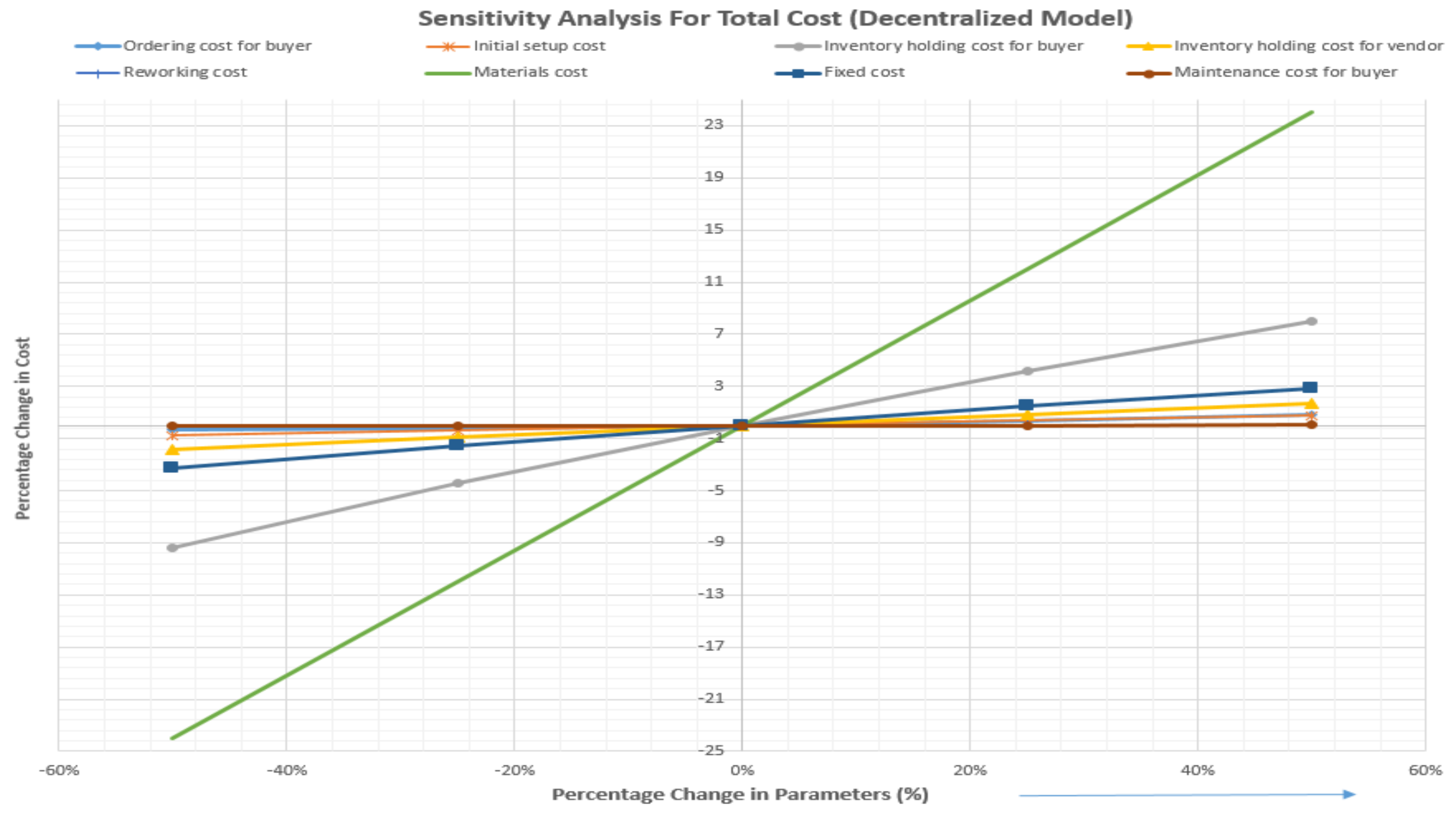
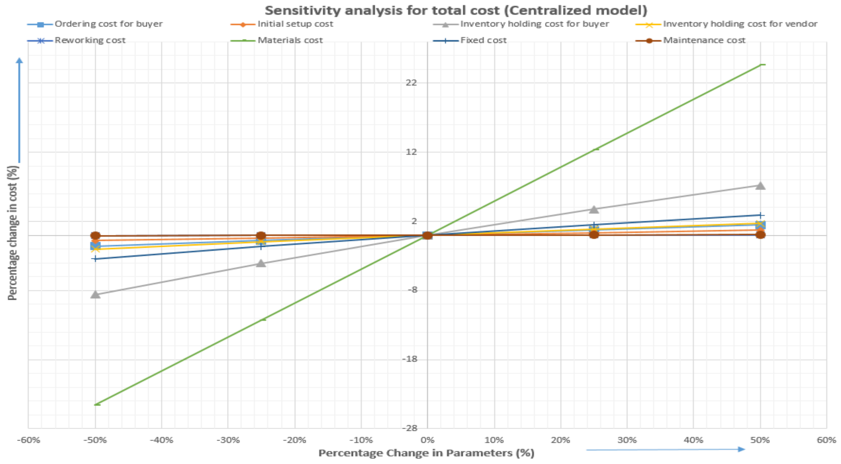
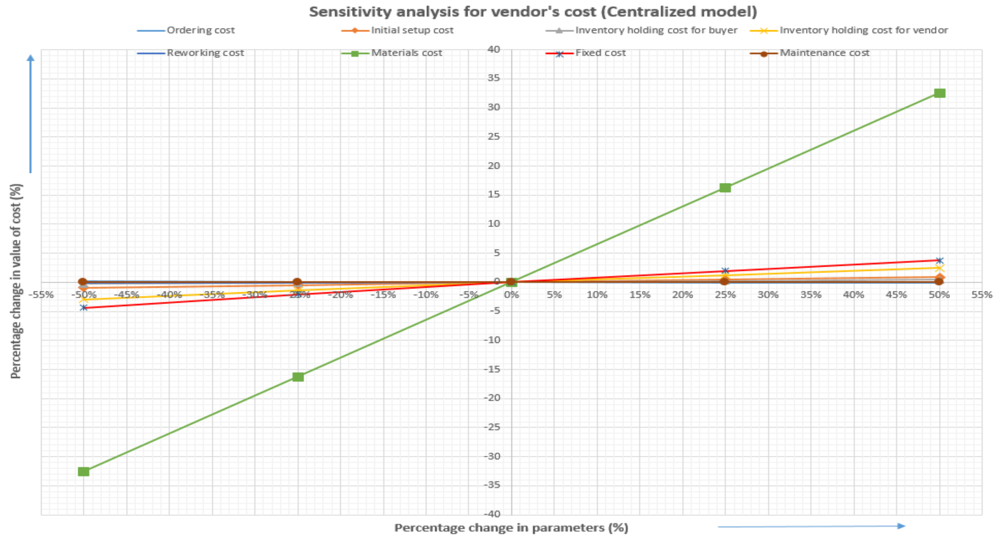
From Table 6 and Table 7, it can be found that the total cost is most sensitive for the raw material cost $C_{mat}$ in both cases, the decentralized and centralized decision making. Figure 2 and Figure 3 show how the total cost increases and decreases with the increase and decrease of major cost parameters in both, decentralized system and centralized system. The second parameter for which total cost is more sensitive is the per unit holding cost for buyer, in both the models. Figure 2 and Figure 3 illustrate how the value of $h_v$ and $h_b$ effect the total cost of the system in centralized and decentralized decision making. While the total cost is more sensitive to the unit holding cost for the buyer as compared to the vendor that is why the SCM managers will apply a single-setup multiple-delivery strategy for replenishment from a vendor to the buyer.

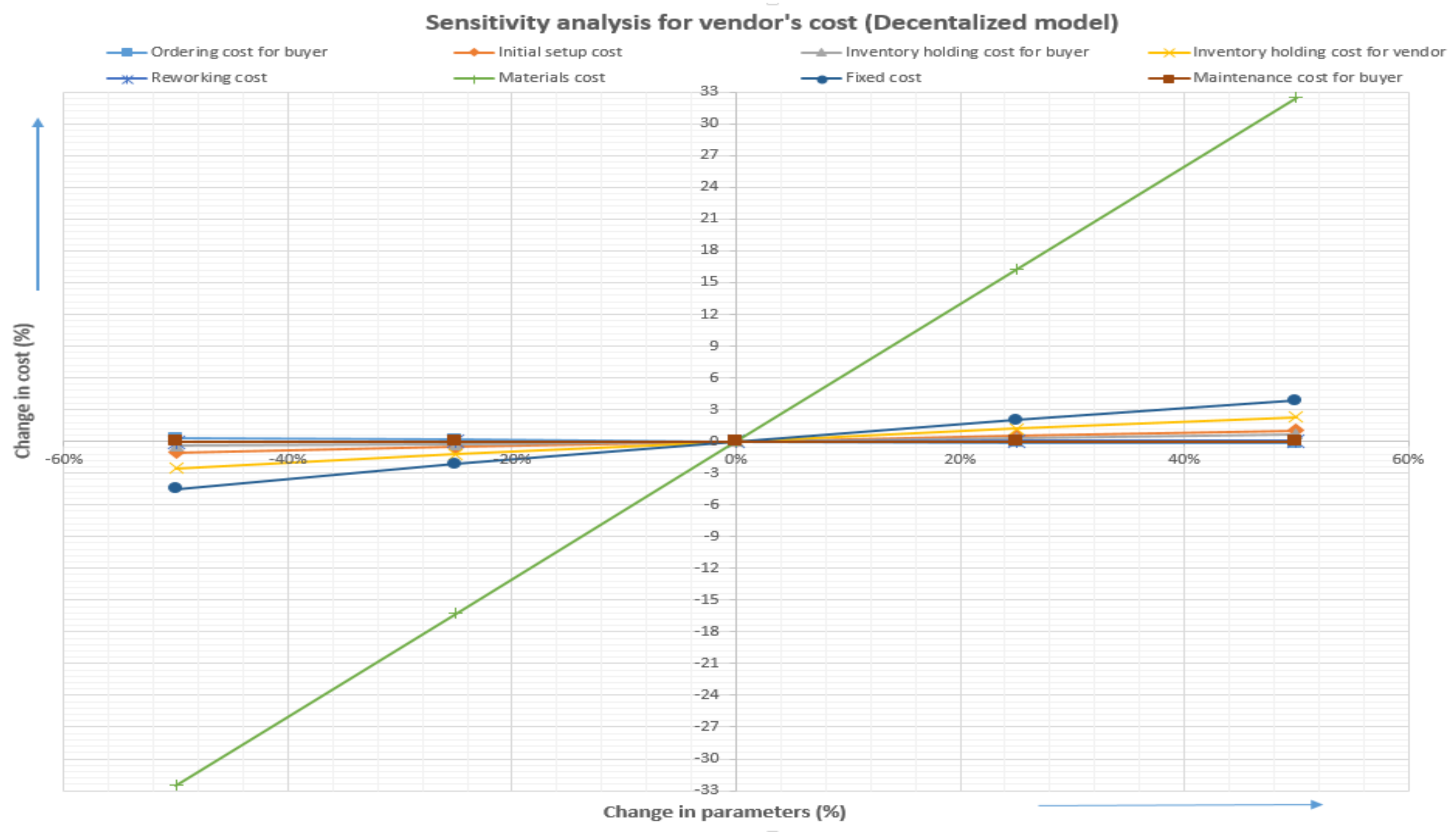
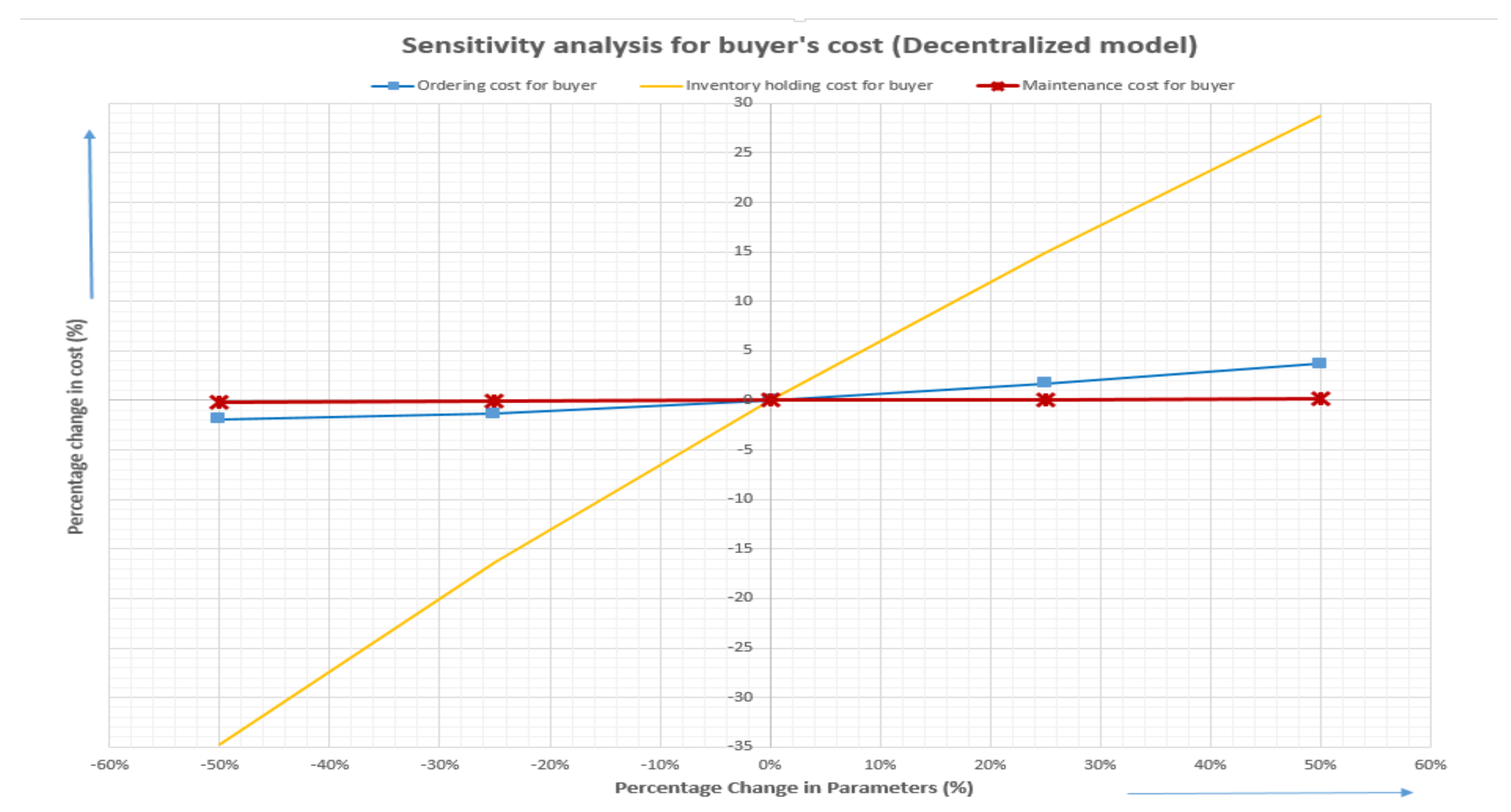
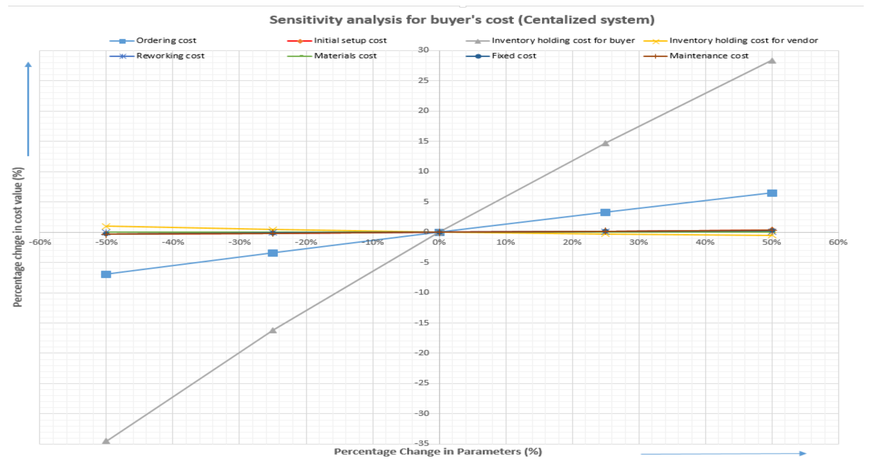
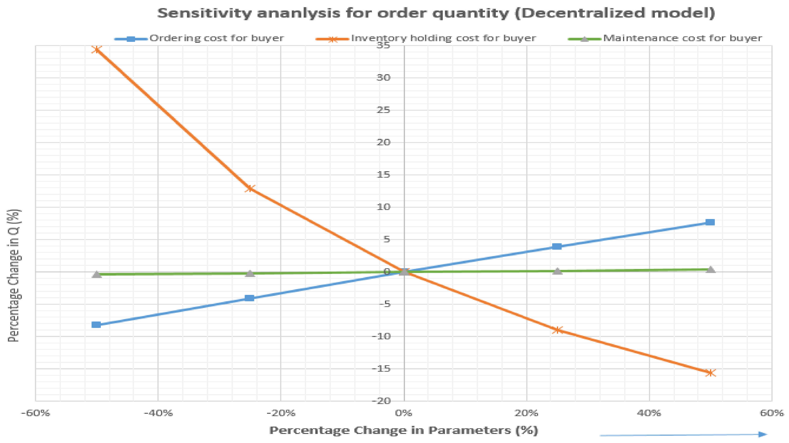
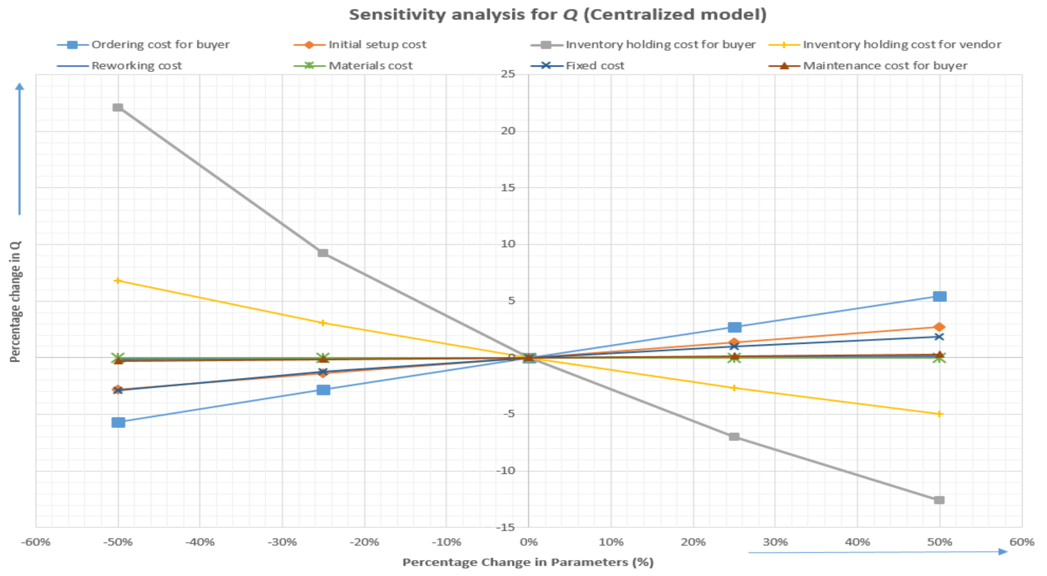
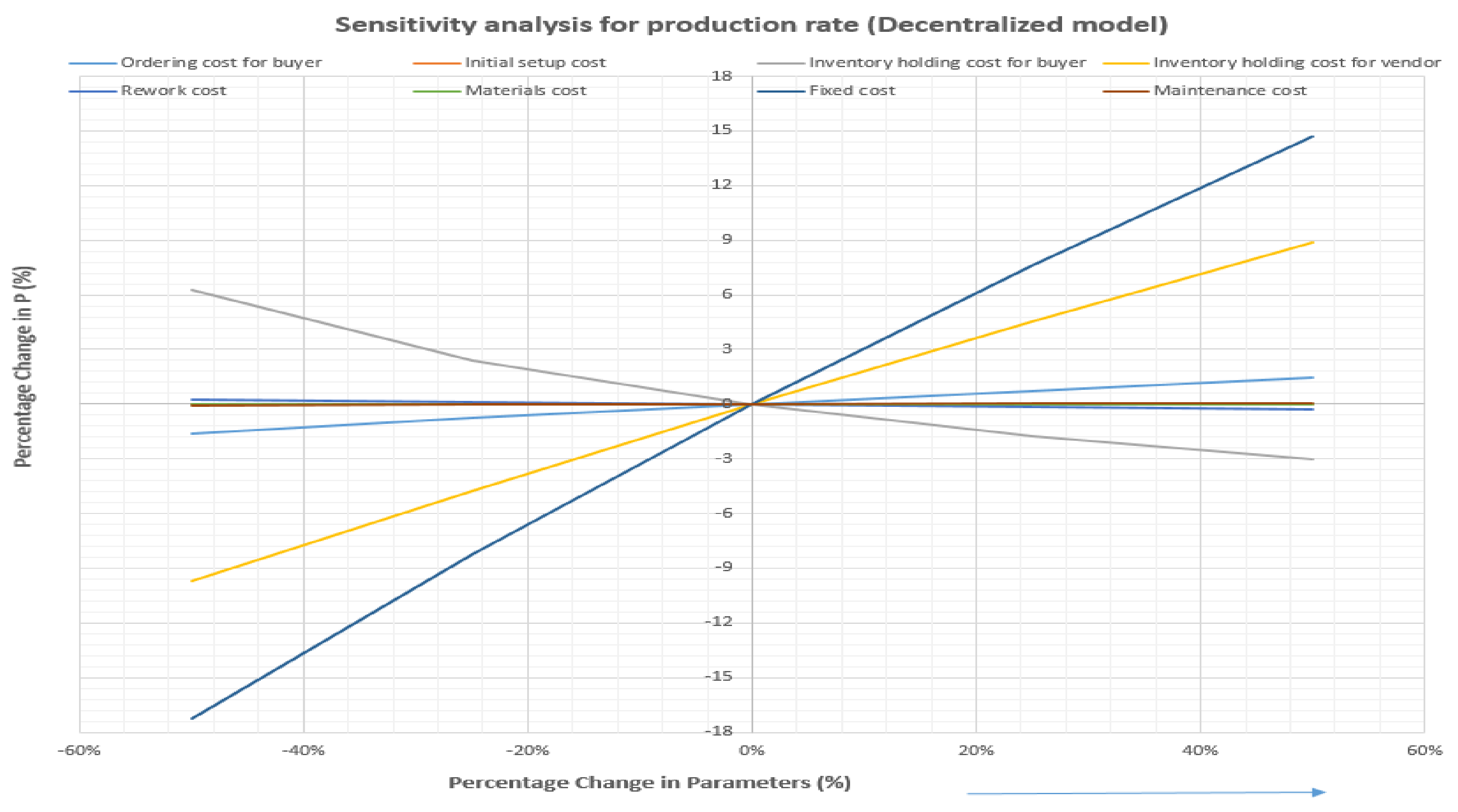
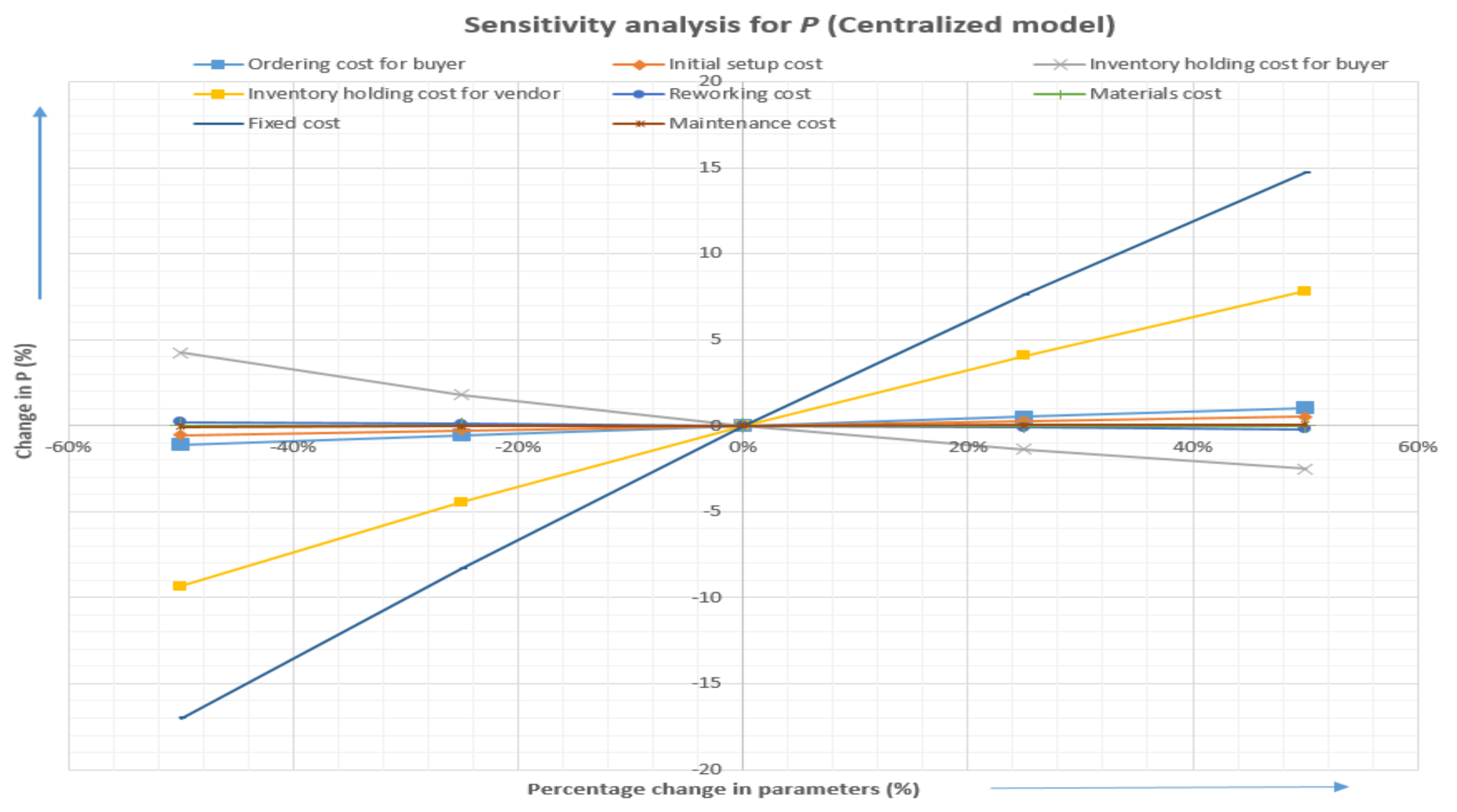
In a similar way, Figure 4 and Figure 5 show the variation in vendor’s cost with the changes in parameter values under the decentralized model and centralized model. This shows the vendor’s cost in both models is directly changing with the changes in values of material cost per product. However, Figure 6 and Figure 7 illustrate the buyer’s cost is more sensitive to the holding cost of buyer and ordering cost per order. In other parametric changes buyer’s cost does not show many variations. The performed sensitivity analysis for order quantity (Q) under the decentralized model and centralized model is shown in Figure 8 and Figure 9, respectively. Under the decentralized model, one can see the order quantity is very sensitive to any changes in ordering cost or the buyer’s holding cost. While in the case of a centralized model it is much more sensitive to the holding cost of the buyer as compared to the other parameter changes. The variations in production rate (P) by changing one parameter and keeping other parameters fixed for a decentralized system are shown in Figure 10. For the centralized system, one can observe the changes in the production rate (P) with the change in parametric values in Figure 11. In centralized decisions, we see the production rate increases with the increase in fixed production cost and vendor’s holding cost. While, the production rate decreases with the increase in holding cost for the buyer. For ordering cost of the buyer and initial setup cost it shows some noticeable changes and does not react much to any changes in the values of other considered cost parameters

7. Research Findings

The research implications of this study are as follows:

• The major managerial insight lies behind the impact of partial backorders and lost sales, for the amount of the permitted shortage. The centralized decision policy gives minimized cost for both participants as compared to the decentralized decision policy.
• An additional investment for setup cost reduction plays a crucial role in the minimization of SCM cost in centralized and decentralized decision policy. The addition of investment is helpful to reduce the setup cost significantly for each setup, which directly has an impact on the SCM cost.
• The controllable production rate provides an opportunity to the vendor for an efficient response to the change in existing and new market demands.
• The optimal lead time is reduced in two ways, by adding the lead time crashing cost and the controllable production rate helps managers to reduce the lead time. The reduction in lead time will affect the customers’ service with a positive impact which will improve the profitability of the entire system.
• Introduced coordination scheme fails to convince the vendor to pay part of lead time crashing cost. It happens due to the lost sales for the amount of the shortage at the buyer’s end. The vendor and the buyer are already getting the lowest cost in centralized decision makings, therefore, both participants make sure the centralized policy works well among them to keep their costs at a minimum.

8. Conclusions

Lead time is considered as a significant component in the inventory management problems. In many real-life situations, the lead time is deemed to be controllable or reducible by an additional crashing cost. Herein, SCM model with a manageable lead time for the Stackelberg game policy and centralized decision policy is proposed. These models are developed by assuming the controllable production rate for the vendor with variable unit production cost, which is dependent on production rate (increase in production rate decreases the unit production cost). Another essential aspect of the manufacturing system, which is considered in these proposed models, is setup cost reduction with initial investments in technology or the workers’ training. The analytical methodology and solution algorithm to get the optimal results are proposed for decentralized Stackelberg game policy and centralized decision policy. In the last part, an asymmetric Nash bargaining model established on the satisfaction levels to obtain the optimal cost sharing or allocation ratio is formulated to bring on both the vendor and the buyer to consent the coordination based centralized model. The provided results of the numerical examples show that controlling shortening lead time can cut down inventory costs. However, the cost allocation or cost sharing model based on the satisfaction levels developed in this paper does not have a significant impact. The insignificance of the coordination policy is due to the two vital factors, lost sales for the percentage of shortages amount, and the vendor and buyer get the minimized cost in the centralized model. Therefore, alternative coordination contracts between vendors and buyers in SCM under the asymmetric information with stochastic conditions can be the point of further research.

The proposed study has several research limitations that should be addressed in future studies. There are different research directions in which this proposed model is extendable, and the immediate extension of this model would be analyzing the model in vendor dominant Stackelberg approach with varying structures of power and multiple products with quantity discounts policy [60]. This model further can be extended to some different directions. With the variable production rate, uncertain demand [61] can be considered with some other fuzzy cost parameters. Uncertain received quantity with quality improvement investment [62,63] can be made to this model for the reduction of the probability of the system moving from in-control to the out-of-control state. Logarithmic investment for ordering cost reduction [62] along with the delay in payments can be considered in future extensions. Another possible extension for this model is to add some more real-life based constraints along with the uncertain environment. A different extension for this model can be considering the deteriorating products for this model. In the future, the model studied can be extended to quality improvements. The vendor makes extra investments for improving the production process quality by reducing the defect rate [64]. Moreover, the coordination mechanism can be developed for multi-buyer single-vendor SCM with the impact of adjustable production rate on the quality of products [7]. Last but not the least, this model can be extended for the controllable carbon emissions rate concerning the variable production rates by investing in green technology [65].

References

- AlDurgam, M.; Adegbola, K.; Glock, C.H. A single-vendor single-manufacturer integrated inventory model with stochastic demand and variable production rate. Int. J. Prod. Econ. 2017, 191, 335–350. [Google Scholar] [CrossRef]
- Saha, S.; Goyal, S. Supply chain coordination contracts with inventory level and retail price dependent demand. Int. J. Prod. Econ. 2015, 161, 140–152. [Google Scholar] [CrossRef]
- Glock, C.H. Lead time reduction strategies in a single-vendor–single-buyer integrated inventory model with lot size-dependent lead times and stochastic demand. Int. J. Prod. Econ. 2012, 136, 37–44. [Google Scholar] [CrossRef]
- Saha, S.; Modak, N.M.; Panda, S.; Sana, S.S. Promotional coordination mechanisms with demand dependent on price and sales efforts. J. Ind. Prod. Eng. 2019, 36, 13–31. [Google Scholar] [CrossRef]
- Malik, A.I.; Kim, B.S. A Constrained Production System Involving Production Flexibility and Carbon Emissions. Mathematics 2020, 8, 275. [Google Scholar] [CrossRef] [Green Version]
- Panda, S.; Saha, S. Optimal production rate and production stopping time for perishable seasonal products with ramp-type time-dependent demand. Int. J. Math. Op. Res. 2010, 2, 657–673. [Google Scholar] [CrossRef]
- Sarkar, B.; Majumder, A.; Sarkar, M.; Kim, N.; Ullah, M. Effects of variable production rate on quality of products in a single-vendor multi-buyer supply chain management. Int. J. Adv. Manuf. Technol. 2018, 99, 567–581. [Google Scholar] [CrossRef]
- Sarkar, M.; Chung, B.D. Flexible work-in-process production system in supply chain management under quality improvement. Int. J. Prod. Res. 2019, 1–18. [Google Scholar] [CrossRef]
- Khouja, M. The economic production lot size model under volume flexibility. Comput. Op. Res. 1995, 22, 515–523. [Google Scholar] [CrossRef]
- Khouja, M.; Mehrez, A. Economic production lot size model with variable production rate and imperfect quality. J. Oper. Res. Soc. 1994, 45, 1405–1417. [Google Scholar] [CrossRef]
- Khouja, M. A Note on ’deliberately Slowing down Output in a Family Production Context’. Int. J. Prod. Res. 1999, 37, 4067–4077. [Google Scholar] [CrossRef]
- Eiamkanchanalai, S.; Banerjee, A. Production lot sizing with variable production rate and explicit idle capacity cost. Int. J. Prod. Econ. 1999, 59, 251–259. [Google Scholar] [CrossRef]
- Giri, B.C.; Yun, W.; Dohi, T. Optimal design of unreliable production–inventory systems with variable production rate. Eur. J. Oper. Res. 2005, 162, 372–386. [Google Scholar] [CrossRef]
- Ayed, S.; Sofiene, D.; Nidhal, R. Joint optimisation of maintenance and production policies considering random demand and variable production rate. Int. J. Prod. Res. 2012, 50, 6870–6885. [Google Scholar] [CrossRef]
- Bouslah, B.; Gharbi, A.; Pellerin, R. Joint optimal lot sizing and production control policy in an unreliable and imperfect manufacturing system. Int. J. Prod. Econ. 2013, 144, 143–156. [Google Scholar] [CrossRef]
- Singh, S.; Prasher, L. A production inventory model with flexible manufacturing, random machine breakdown and stochastic repair time. Int. J. Ind. Eng. Comput. 2014, 5, 575–588. [Google Scholar] [CrossRef] [Green Version]
- Glock, C.H. Batch sizing with controllable production rates. Int. J. Prod. Res. 2010, 48, 5925–5942. [Google Scholar] [CrossRef] [Green Version]
- Glock, C.H. Batch sizing with controllable production rates in a multi-stage production system. Int. J. Prod. Res. 2011, 49, 6017–6039. [Google Scholar] [CrossRef]
- Dey, B.K.; Pareek, S.; Tayyab, M.; Sarkar, B. Autonomation policy to control work-in-process inventory in a smart production system. Int. J. Prod. Res. 2020, 1–23. [Google Scholar] [CrossRef]
- Sarkar, B.; Omair, M.; Kim, N. A cooperative advertising collaboration policy in supply chain management under uncertain conditions. Appl. Soft Comput. 2020, 88, 105948. [Google Scholar] [CrossRef]
- Glock, C.H. The joint economic lot size problem: A review. Int. J. Prod. Econ. 2012, 135, 671–686. [Google Scholar] [CrossRef]
- Goyal, S. An integrated inventory model for a single supplier-single customer problem. Int. J. Prod. Res. 1977, 15, 107–111. [Google Scholar] [CrossRef]
- Banerjee, A. A joint economic-lot-size model for purchaser and vendor. Decis. Sci. 1986, 17, 292–311. [Google Scholar] [CrossRef]
- Lu, L. A one-vendor multi-buyer integrated inventory model. Eur. J. Oper. Res. 1995, 81, 312–323. [Google Scholar] [CrossRef]
- Goyal, S.K. A one-vendor multi-buyer integrated inventory model: A comment. Eur. J. Oper. Res. 1995, 82, 209–210. [Google Scholar] [CrossRef]
- Hill, R.M. The optimal production and shipment policy for the single-vendor singlebuyer integrated production-inventory problem. Int. J. Prod. Res. 1999, 37, 2463–2475. [Google Scholar] [CrossRef]
- Huang, C.K. An optimal policy for a single-vendor single-buyer integrated production–inventory problem with process unreliability consideration. Int. J. Prod. Econ. 2004, 91, 91–98. [Google Scholar] [CrossRef]
- Wee, H.M.; Widyadana, G.A. Single-vendor single-buyer inventory model with discrete delivery order, random machine unavailability time and lost sales. Int. J. Prod. Econ. 2013, 143, 574–579. [Google Scholar] [CrossRef]
- Pan, J.C.H.; Yang, J.S. A study of an integrated inventory with controllable lead time. Int. J. Prod. Res. 2002, 40, 1263–1273. [Google Scholar] [CrossRef]
- Ouyang, L.Y.; Wu, K.S.; Ho, C.H. Integrated vendor–buyer cooperative models with stochastic demand in controllable lead time. Int. J. Prod. Econ. 2004, 92, 255–266. [Google Scholar] [CrossRef]
- Ye, F.; Xu, X. Cost allocation model for optimizing supply chain inventory with controllable lead time. Comput. Ind. Eng. 2010, 59, 93–99. [Google Scholar] [CrossRef]
- Kunter, M. Coordination via cost and revenue sharing in manufacturer–retailer channels. Eur. J. Oper. Res. 2012, 216, 477–486. [Google Scholar] [CrossRef]
- Heydari, J. Lead time variation control using reliable shipment equipment: An incentive scheme for supply chain coordination. Transp. Res. Part E Logist. Transp. Rev. 2014, 63, 44–58. [Google Scholar] [CrossRef]
- Heydari, J. Coordinating supplier’s reorder point: A coordination mechanism for supply chains with long supplier lead time. Comput. Oper. Res. 2014, 48, 89–101. [Google Scholar] [CrossRef]
- Heydari, J.; Mahmoodi, M.; Taleizadeh, A.A. Lead time aggregation: A three-echelon supply chain model. Transp. Res. Part E Logist. Transp. Rev. 2016, 89, 215–233. [Google Scholar] [CrossRef] [Green Version]
- Basiri, Z.; Heydari, J. A mathematical model for green supply chain coordination with substitutable products. J. Clean. Prod. 2017, 145, 232–249. [Google Scholar] [CrossRef] [Green Version]
- Moon, I.; Jeong, Y.J.; Saha, S. Investment and coordination decisions in a supply chain of fresh agricultural products. Oper. Res. 2018, 1–25. [Google Scholar] [CrossRef]
- Malik, A.I.; Sarkar, B. Coordinating Supply-Chain Management under Stochastic Fuzzy Environment and Lead-Time Reduction. Mathematics 2019, 7, 480. [Google Scholar] [CrossRef] [Green Version]
- Daryanto, Y.; Wee, H.M.; Widyadana, G.A. Low carbon supply chain coordination for imperfect quality deteriorating items. Mathematics 2019, 7, 234. [Google Scholar] [CrossRef] [Green Version]
- Xin, C.; Chen, X.; Chen, H.; Chen, S.; Zhang, M. Green Product Supply Chain Coordination Under Demand Uncertainty. IEEE Access 2020, 8, 25877–25891. [Google Scholar] [CrossRef]
- Gallego, G.; Moon, I. The distribution free newsboy problem: Review and extensions. J. Oper. Res. Soc. 1993, 44, 825–834. [Google Scholar] [CrossRef]
- Scarf, H.; Arrow, K.; Karlin, S. A min-max solution of an inventory problem. Stud. Math. Theory Invent. Prod. 1958, 10, 201. [Google Scholar]
- Moon, I.; Choi, S. Technical notea note on lead time and distributional assumptions in continuous review inventory models. Comput. Oper. Res. 1998, 25, 1007–1012. [Google Scholar] [CrossRef]
- Tajbakhsh, M.M. On the distribution free continuous-review inventory model with a service level constraint. Comput. Ind. Eng. 2010, 59, 1022–1024. [Google Scholar] [CrossRef]
- Moon, I.; Shin, E.; Sarkar, B. Min–max distribution free continuous-review model with a service level constraint and variable lead time. Appl. Math. Comput. 2014, 229, 310–315. [Google Scholar] [CrossRef]
- Sarkar, B.; Chaudhuri, K.; Moon, I. Manufacturing setup cost reduction and quality improvement for the distribution free continuous-review inventory model with a service level constraint. J. Manuf. Syst. 2015, 34, 74–82. [Google Scholar] [CrossRef]
- Shin, D.; Guchhait, R.; Sarkar, B.; Mittal, M. Controllable lead time, service level constraint, and transportation discounts in a continuous review inventory model. Rairo OR 2016, 50, 921–934. [Google Scholar] [CrossRef]
- Malik, A.I.; Sarkar, B. A distribution-free model with variable setup cost, backorder price discount and controllable lead time. DJ J. Eng. Appl. Math. 2018, 4, 58–69. [Google Scholar] [CrossRef]
- Malik, A.I.; Sarkar, B. Optimizing a Multi-Product Continuous-Review Inventory Model With Uncertain Demand, Quality Improvement, Setup Cost Reduction, and Variation Control in Lead Time. IEEE Access 2018, 6, 36176–36187. [Google Scholar] [CrossRef]
- Moon, I.; Yoo, D.K.; Saha, S. The distribution-free newsboy problem with multiple discounts and upgrades. Math. Problems Eng. 2016, 2016, 1–11. [Google Scholar] [CrossRef] [Green Version]
- Guchhait, R.; Dey, B.K.; Bhuniya, S.; Ganguly, B.; Mandal, B.; Bachar, R.K.; Sarkar, B.; Wee, H.; Chaudhuri, K. Investment for process quality improvement and setup cost reduction in an imperfect production process with warranty policy and shortages. RAIRO-Oper. Res. 2020, 54, 251–266. [Google Scholar] [CrossRef] [Green Version]
- Sarmah, S.; Acharya, D.; Goyal, S. Buyer vendor coordination models in supply chain management. Eur. J. Oper. Res. 2006, 175, 1–15. [Google Scholar] [CrossRef]
- Kanda, A.; Deshmukh, S. Supply chain coordination: Perspectives, empirical studies and research directions. Int. J. Prod. Econ. 2008, 115, 316–335. [Google Scholar]
- Sarkar, B.; Saren, S. Product inspection policy for an imperfect production system with inspection errors and warranty cost. Eur. J. Oper. Res. 2016, 248, 263–271. [Google Scholar] [CrossRef]
- Huang, C.K.; Cheng, T.; Kao, T.; Goyal, S. An integrated inventory model involving manufacturing setup cost reduction in compound Poisson process. Int. J. Prod. Res. 2011, 49, 1219–1228. [Google Scholar] [CrossRef]
- Ouyang, L.Y.; Yeh, N.C.; Wu, K.S. Mixture inventory model with backorders and lost sales for variable lead time. J. Oper. Res. Soc. 1996, 47, 829–832. [Google Scholar] [CrossRef]
- Nash, J.F., Jr. The bargaining problem. Econom. J. Econom. Soc. 1950, 18, 155–162. [Google Scholar] [CrossRef]
- Harsanyi, J.C.; Selten, R. A generalized Nash solution for two-person bargaining games with incomplete information. Manag. Sci. 1972, 18, 80–106. [Google Scholar] [CrossRef]
- Sarkar, B. Supply chain coordination with variable backorder, inspections, and discount policy for fixed lifetime products. Math. Problems Eng. 2016, 2016, 1–14. [Google Scholar] [CrossRef] [Green Version]
- Noh, J.S.; Kim, J.S.; Sarkar, B. Stochastic joint replenishment problem with quantity discounts and minimum order constraints. Oper. Res. 2019, 19, 151–178. [Google Scholar] [CrossRef]
- Ouyang, L.Y.; Yao, J.S. A minimax distribution free procedure for mixed inventory model involving variable lead time with fuzzy demand. Comput. Oper. Res. 2002, 29, 471–487. [Google Scholar] [CrossRef]
- Porteus, E.L. Optimal lot sizing, process quality improvement and setup cost reduction. Oper. Res. 1986, 34, 137–144. [Google Scholar] [CrossRef]
- Cheikhrouhou, N.; Sarkar, B.; Ganguly, B.; Malik, A.I.; Batista, R.; Lee, Y.H. Optimization of sample size and order size in an inventory model with quality inspection and return of defective items. Ann. Oper. Res. 2018, 271, 445–467. [Google Scholar] [CrossRef] [Green Version]
- Sarkar, B.; Mandal, B.; Sarkar, S. Quality improvement and backorder price discount under controllable lead time in an inventory model. J. Manuf. Syst. 2015, 35, 26–36. [Google Scholar] [CrossRef]
- Mishra, U.; Wu, J.Z.; Sarkar, B. A sustainable production-inventory model for a controllable carbon emissions rate under shortages. J. Cleaner Prod. 2020, 256, 120268. [Google Scholar] [CrossRef]
Figure 1.
Lead time crashing cost calculations.
Figure 2.
Sensitivity analysis: total cost versus change in parameters under decentralized model.
Figure 3.
Sensitivity analysis: total cost versus change in parameters under centralized model.
Figure 4.
Sensitivity analysis: vendor’s cost versus change in parameters under decentralized model.
Figure 5.
Figure 6.
Sensitivity analysis: buyer’s cost versus change in parameters under decentralized model.
Figure 7.
Figure 8.
Sensitivity analysis: order quantity (Q) versus change in parameters under decentralized model.
Figure 9.
Figure 10.
Sensitivity analysis: production rate (P) versus change in parameters under decentralized model.
Figure 11.