Construction of Different Types Analytic Solutions for the Zhiber-Shabat Equation


1
Department of Actuary, Faculty of Science, Firat University, Elazig 23200, Turkey
2
Department of Computer Engineering, Faculty of Engineering, Ardahan University, Ardahan 75000, Turkey
3
Department of Basic Sciences, University of Engineering and Technology, Peshawar 25000, Pakistan
4
School of Mathematics and Information Science, Henan Polytechnic University, Jiaozuo 454000, China
*
Author to whom correspondence should be addressed.
†
These authors contributed equally to this work.
Mathematics 2020, 8(6), 908; https://doi.org/10.3390/math8060908
Submission received: 10 May 2020
/
Revised: 1 June 2020
/
Accepted: 2 June 2020
/
Published: 3 June 2020
(This article belongs to the Special Issue Differential/Difference Equations: Mathematical Modeling, Oscillation and Applications)
Abstract
:In this paper, a new solution process of -expansion and -expansion methods has been proposed for the analytic solution of the Zhiber-Shabat (Z-S) equation. Rather than the classical -expansion method, a solution function in different formats has been produced with the help of the proposed process. New complex rational, hyperbolic, rational and trigonometric types solutions of the Z-S equation have been constructed. By giving arbitrary values to the constants in the obtained solutions, it can help to add physical meaning to the traveling wave solutions, whereas traveling wave has an important place in applied sciences and illuminates many physical phenomena. 3D, 2D and contour graphs are displayed to show the stationary wave or the state of the wave at any moment with the values given to these constants. Conditions that guarantee the existence of traveling wave solutions are given. Comparison of -expansion method and -expansion method, which are important instruments in the analytical solution, has been made. In addition, the advantages and disadvantages of these two methods have been discussed. These methods are reliable and efficient methods to obtain analytic solutions of nonlinear evolution equations (NLEEs).
1. Introduction
The analysis of analytic solutions of nonlinear evolution equations (NLEEs) plays a significant role in the study of nonlinear physical phenomena. Various techniques have been tried to obtained analytic solutions, such as the sine–cosine method [1], extended sinh-Gordon equation expansion method [2,3], -expansion method [4,5], improved Bernoulli sub-equation function method [6], variational iteration algorithm-II [7,8,9], sub equation method [10], collocation method [11,12], -expansion method [13,14,15], first integral method [16], adomian decomposition methods [17,18,19], hirota bilinear method [20], modified variational iteration algorithms [21,22,23,24], homotopy perturbation method [25], residual power series method [26], -expansion method [27] and so on [28,29,30,31,32,33,34,35,36,37,38].
In this study, our main purpose is to obtain the traveling wave solutions of the evolution equations in nonlinear dynamics. As it is known, scientific studies take place gradually. The first step is to examine a physical event, the second step is to model the event, the third step is to produce the solution of the model and the fourth step is to load the produced solution into physical meaning. In this article, to produce the solution in the third stage and to prepare for the fourth stage. As it is known, in soliton theory, it will be much more valuable if solitons gain physical meaning. For example, today, the pandemic patients that affect the world may represent a stationary wave on a graph consisting of numerical data related to parameters such as number of patients and number of tests. Employees on this subject can relate to the solutions we will offer in this study. We consider the Zhiber-Shabat (Z-S) equation [39]
where are arbitrary constants. When , Equation (1) gives the well-known sinh–Gordon equation, while, , gives the Dodd–Bullough–Mikhailov (DBM) equation. However, for Equation (1) reduced to the Tzitzeica–Dodd–Bullough (TDB) equation, while for , gives the Liouville equation. These equations play an effective role in various scientific applications such as fluid dynamics, solid state physics, nonlinear optics and chemical kinetics. When the analytical solution of Equation (1) is found, the solutions of the sinh–Gordon, DBM, TDB and the Liouville equations can also be obtained.
Many researchers have investigated the Z-S equations and discussed its applications in different field of science and engineering. Some of these investigations are as follows: various types of solution for the Z-S equation are obtained [40] by using qualitative theory of polynomial differential system, while qualitative behavior and exact travelling wave solutions of the Z-S equation are obtained in [41]. Analytic solutions of the Z-S equation are obtained using the -expansion method [42], exponential rational function method [43], while exact solutions of it are obtained using bifurcation theory and method of phase portraits analysis [44].
In the current work, we are interested in constructing exact solutions of the Zhiber-Shabat (Z-S) equation using -expansion method and -expansion method. The solutions of the equation have not been studied with either method. In this study, both to provide the literature with the solution produced by these methods and to discuss the advantages and disadvantages of the methods.
2. -Expansion Method
Consider a general form of NLEEs as
Let where w is a constant speed of the wave. After using transformation, it can be converted into the following nonlinear ODE for :
The solution of Equation (3) is assumed to have the form
where are constants and provides the following second order IODE
where, and are constants to be determined after,
where A is an integral constant. If the desired derivatives of the Equation (4) are calculated and substituting in the Equation (3), a polynomial with the argument is attained. An algebraic equation system is created by equalizing the coefficients of this polynomial to zero. These equations are solved with the help of the package program and put into place in the default Equation (3) solution function. Finally, the solutions of Equation (1) are obtained.
3. -Expansion Method
Consider the following general form of NLEEs
If where w is a constant, when transmutation is applied to Equation (7), it becomes a NLODE and this equation may be written as:
Complexity can be reduced by integrating Equation (8). By the nature of this method, is a quadratic function ODE solution,
Furthermore, to provide operational aesthetics as and . We may write derivatives of functions defined here;
We can offer the behavior of solution function Equation (9) according to the state of , taking into account the equations given by the Equation (10).
Equation (12) is written.
ii: If
here and are reel numbers. Considering Equation (13), there is following equation;
iii: If
here and are reel numbers. Considering Equation (15), there is following equation;
In terms of and polynomials, solution of Equation (8) is;
In this study, we reorganized the solution function in classical -expansion method as Equation (17) with the logic of solution functions of and -expansion methods. This logic is considered together with the classical -expansion method and the method can be developed in future studies and different solutions can be offered.
Wherein, and counts then are constants to be determined. m is a positive equilibrium term that may be attained by comparing the maximum order derivative and the maximum order nonlinear term in Equation (8). If Equation (17) is written in Equation (8) with Equations (10), (12), (14) or (16), a polynomial function associated with and is written. Each term coefficient of of the attained polynomial functions are equated to zero and a system algebraic equations is attained for and . The required coefficients are obtained by solving the algebraic equation with the help of computer package programs. These coefficients found are written in Equation (17) and solution function of Equation (8) is obtained and if transmutation is employed in reverse order, we will attain analytic solution of Equation (7).
4. Solutions of the (Z-S) Equation Using -Expansion Method
We consider Equation (1). Using transmutation we obtain
where w is the wave speed. To implement this method, we use transmutation and , Equation (18) becomes
In Equation (19), we find balancing term and in Equation (4), the following situation is obtained:
where unknown constants to be determined later. Replacing Equation (20) into Equation (19) and the coefficients of the algebraic Equation (1) are equal to zero, we can establish the following algebraic equation systems
Case I.
considering Equation (6), substituting Equation (22) into Equation (20), the following solution is attained
In addition, if Equation (23) is written instead of transformation, the analytical solution of Equation (1) is as follows,
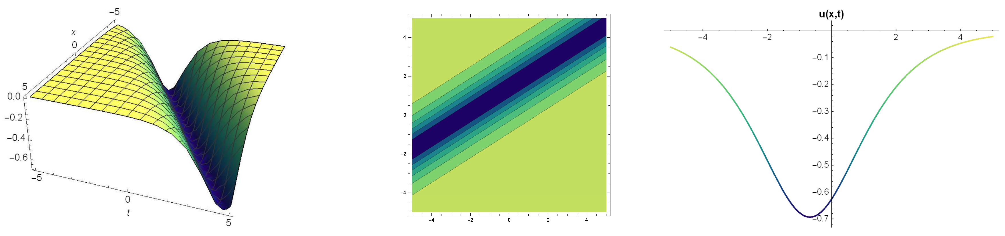
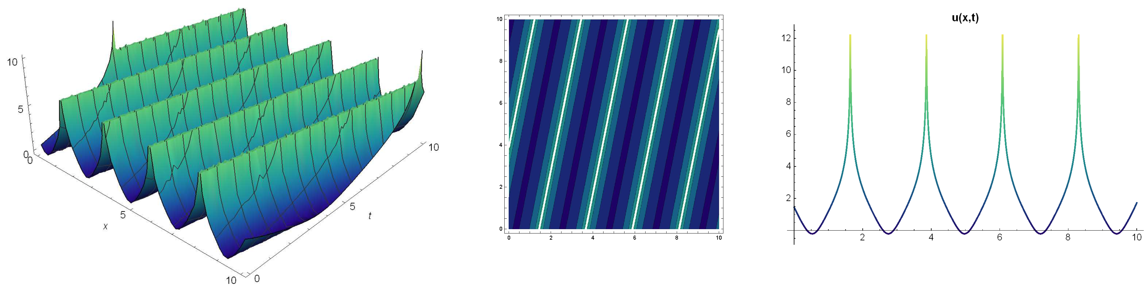
The hyperbolic traveling wave solution of Equation (24) produced from the -expansion method is as in Figure 1.
Case II.
considering Equation (6), replacing Equation (25) into Equation (20), the following solution is attained
5. Solutions of the (Z-S) Equation Using -Expansion Method
We consider Equation (1). Using transmutation , we get
To apply this method, we use transmutation and , Equation (28) becomes
In Equation (29), we find balancing term and in Equation (10), the following situation is obtained
where constants to be determined are unknown. Replacing Equation (30) into Equation (29) and the coefficients of the algebraic Equation (1) are equal to zero, we can establish the following algebraic equation systems
Our aim with the computer package program was reaching the solutions of system (31) and we attained the following situations.
If
Case I:
considering Equation (6), replacing Equation (32) into Equation (30), the following solution is attained
In addition, if Equation (33) is written instead of transformation, the hyperbolic traveling wave solution of Equation (1) is as follows,
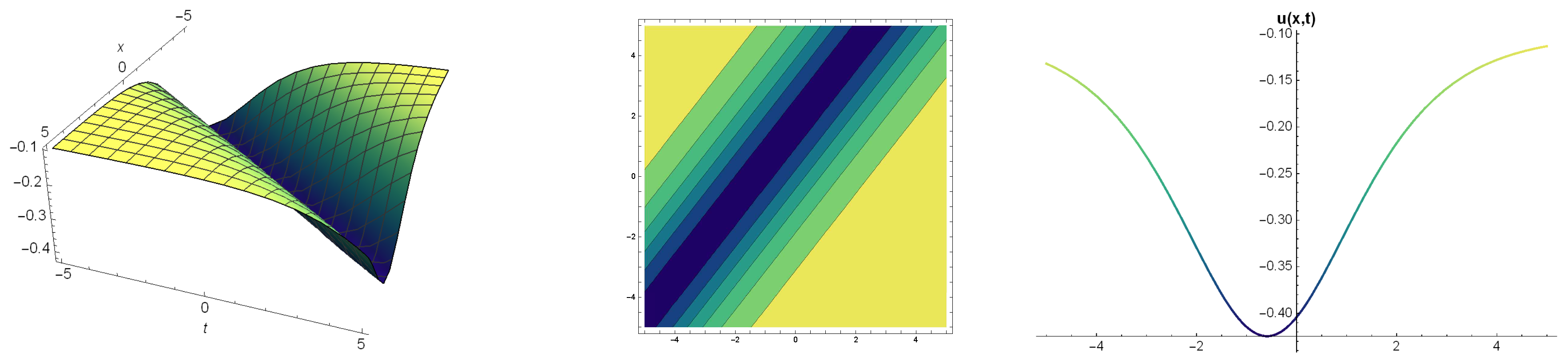
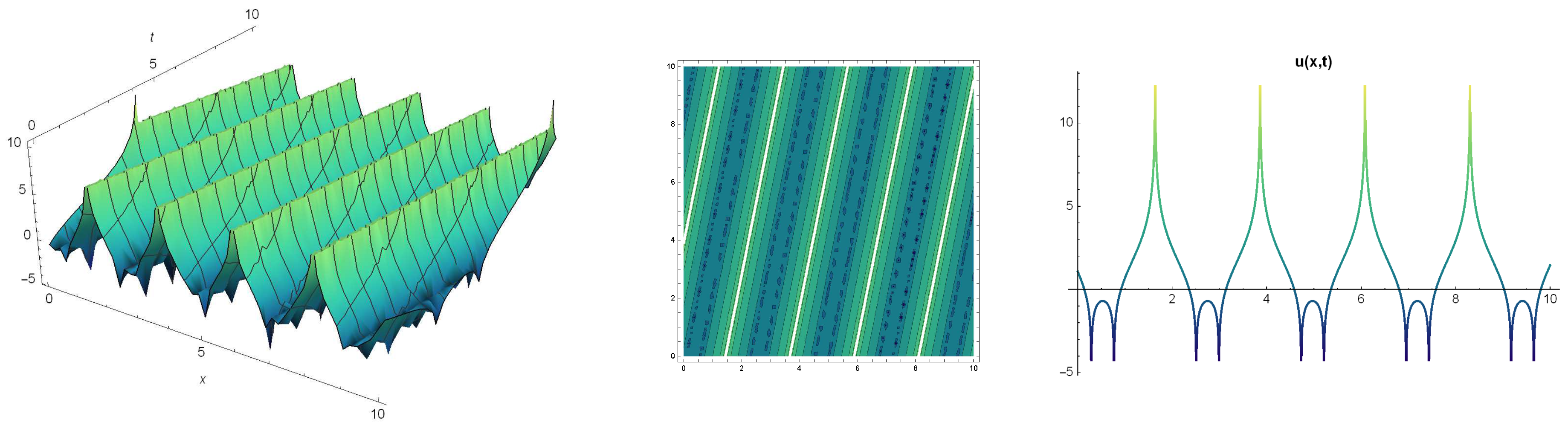
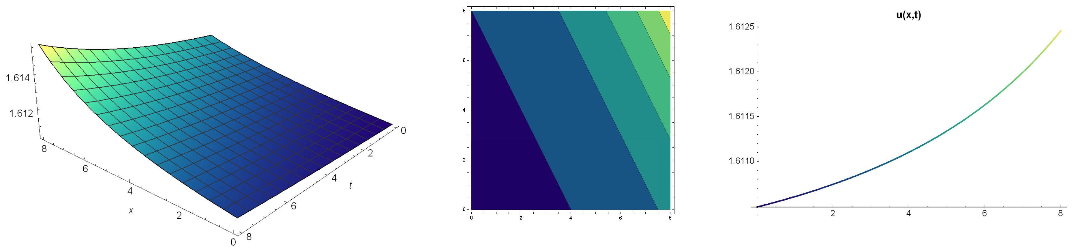
The hyperbolic traveling wave solution of Equation (34) produced from the -expansion method is as in Figure 3.
Case II:
considering Equation (6), replacing Equation (35) into Equation (30), the following solution is attained
In addition, if Equation (36) is written instead of transformation, the hyperbolic traveling wave solution of Equation (1) is as follows,
The hyperbolic traveling wave solution of Equation (37) produced from the -expansion method is as in Figure 4.
If
Case III:
considering Equation (6), replacing Equation (38) into Equation (30), the following solution is attained
In addition, if Equation (39) is written instead of transformation, the trigonometric traveling wave solution of Equation (1) is as follows,
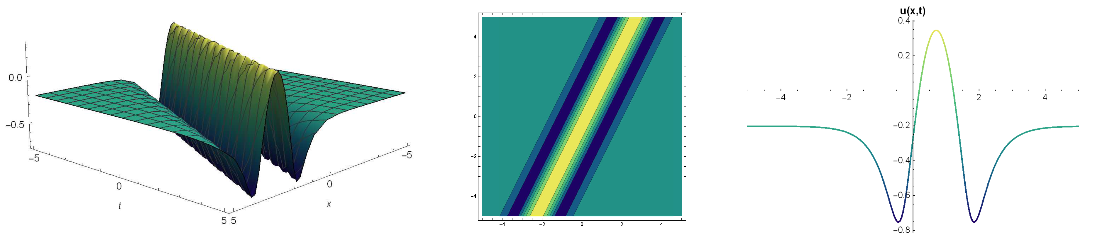
The trigonometric traveling wave solution of Equation (40) produced from the -expansion method is as in Figure 5.
Case IV:
considering Equation (6), replacing Equation (41) into Equation (30), the following solution is attained
In addition, if Equation (42) is written instead of transformation, the analytical solution of Equation (1) is as follows,
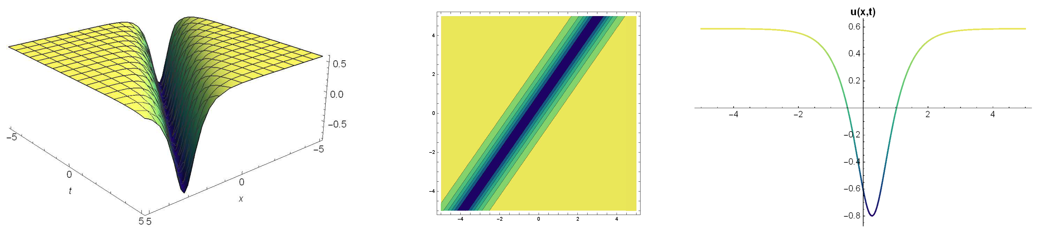
The trigonometric traveling wave solution of Equation (43) produced from the -expansion method is as in Figure 6.
If
Case V:
considering Equation (6), replacing Equation (44) into Equation (30), the following solution is attained
In addition, if Equation (45) is written instead of transformation, the complex analytical solution of Equation (1) is as follows,
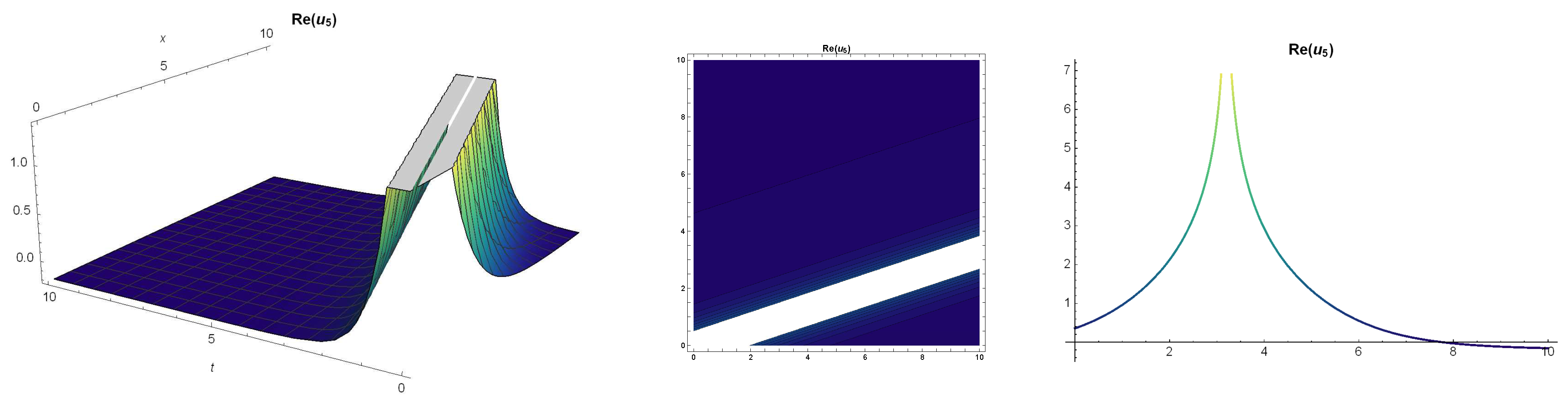
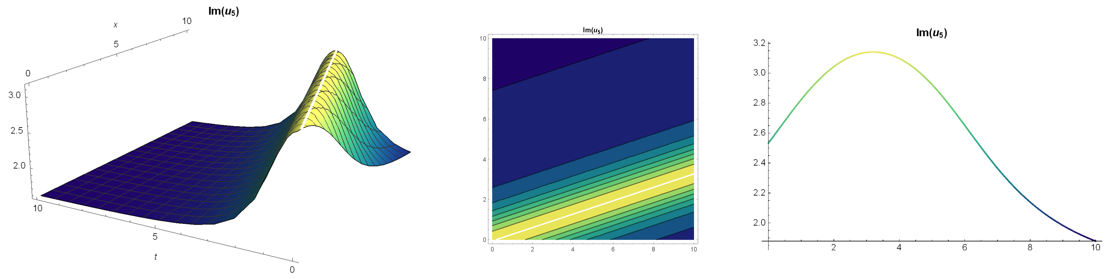
The complex analytical solution of Equation (46) produced from the -expansion method is as in Figure 7 and Figure 8.
Case VI:
considering Equation (6), replacing Equation (47) into Equation (30), the following solution is attained
6. Results and Discussion
There are various methods for obtaining the exact solution of NLEEs. Analytic solutions of the Z-S equations were successfully constructed by using both methods. When transformation is performed in both methods, solution functions are logarithmic. This is a result of the exponential functions in the structure of the Z-S equation. In different cases of p, q, r coefficients of Z-S equation, this equation is recognized by a different name. The main purpose of this article is to present the solution of Z-S equation and also to solve the equations of the sinh–Gordon, (DBM), (TDB) and the Liouville equations. For example; The Z-S equation for is called the Liouville equation. In this study, if the values in Equation (24) are written, the traveling wave solution of the Liouville equation is obtained as
Similarly, the solutions of the sinh–Gordon, DBM, TDB and Liouville equations can be obtained by using both the methods. The V solution described above is presented in hyperbolic form in -expansion method, and in hyperbolic, trigonometric and rational forms in -expansion method. In this case, -expansion method is advantageous in terms of solution. However, in -expansion method, the process complexity is higher. This can be observed in the system Equation (31), -expansion method is more advantageous in terms of process. 2D, 3D and contour graphics which we consider will help in traveling wave solutions which have considerable importance in applied sciences, are presented. In order to draw these graphs, real values are given to arbitrary constants in the analytical solution.
This problem contains the properties of many equations. For the different states of the coefficients, to offer the solution of the equation which includes equations with different names, also to offer the solution of the subclass equations. It is known that each equation has different meanings. For example, with the interaction of solitons produced by sinh-Gordon equation, kink and antikink solutions came to the fore. We can make the same comments for the solutions obtained in these studies for. In this case, the equation we dealt with is the umbrella task. It makes the wave solutions valuable because it will carry the properties of the equations under the umbrella. The most important factor that stands out in this study is to take a different solutions from the solution in classical -expansion method. This results in obtaining different types of traveling wave solutions from the classical method. It also creates a basis for a new study. This is an improved method that can produce different solutions by adding the solution we offer with the Equation (17) to the classical solution. Because the Equation (17) presented and the equilibrium term 2 in the equation discussed are different from the solutions offered in the classical -expansion method. Different types of solutions were obtained with both methods and both methods can be used as important instruments to get traveling wave solution for many different NLEEs.
7. Conclusions
In this article, we have applied the -expansion and -expansion methods to derive analytic solutions for the Zhiber-Shabat equation. The solutions obtained are complex rational, hyperbolic, rational and trigonometric type traveling wave solutions. The 2D, 3D and contour graphics of these solutions were presented by giving value to arbitrary parameters. These graphs represent the stationary wave at any given moment. As it is very difficult to obtain the solutions of NLEEs, in this study traveling wave solutions of Zhiber-Shabat equation are presented applying two complex methods using many complex operations and transformations. These are very effective and powerful methods for obtaining analytical solutions and can be used to obtain solutions of many mathematical models representing physical phenomena. The accuracy of the attained solutions has been assured by putting them back into the original equations with the help of the computer package program.
Author Contributions
Conceptualization, A.Y.; data curation, A.Y. and H.D.; formal analysis, H.A.; funding acquisition, S.-W.Y.; investigation, H.D.; methodology, A.Y.; software, H.D.; supervision, A.Y.; writing—original draft, H.A.; writing—review and editing, S.-W.Y. All authors have read and agreed to the published version of the manuscript.
Funding
This work was supported by National Natural Science Foundation of China (No. 71601072) and Key Scientific Research Project of Higher Education Institutions in Henan Province of China (No. 20B110006).
Acknowledgments
The authors thank the Editor-in-Chief and unknown referees for the fruitful comments and significant remarks that helped them in improving the quality and readability of the paper, which led to a significant improvement of the paper.
Conflicts of Interest
The authors declare no conflict of interest.
References
- Wazwaz, A.M. A sine-cosine method for handlingnonlinear wave equations. Math. Comput. Model. 2004, 40, 499–508. [Google Scholar] [CrossRef]
- Baskonus, H.M.; Sulaiman, T.A.; Bulut, H.; Aktürk, T. Investigations of dark, bright, combined dark-bright optical and other soliton solutions in the complex cubic nonlinear Schrödinger equation with δ-potential. Superlattices Microstruct. 2018, 115, 19–29. [Google Scholar] [CrossRef]
- Cattani, C.; Sulaiman, T.A.; Baskonus, H.M.; Bulut, H. On the soliton solutions to the Nizhnik-Novikov-Veselov and the Drinfel’d-Sokolov systems. Opt. Quantum Electron. 2018, 50. [Google Scholar] [CrossRef]
- Yokuş, A.; Kaya, D. Traveling wave solutions of some nonlinear partial differential equations by using extended-expansion method. İstanbul Ticaret Üniversitesi Fen Bilimleri Dergisi 2015, 28, 85–92. [Google Scholar]
- Durur, H. Different types analytic solutions of the (1+1)-dimensional resonant nonlinear Schrödinger’s equation using (G′/G)-expansion method. Mod. Phys. Lett. B 2020, 34. [Google Scholar] [CrossRef]
- Bulut, H.; Yel, G.; Başkonuş, H.M. An application of improved Bernoulli sub-equation function method to the nonlinear time-fractional burgers equation. Turk. J. Math. Comput. Sci. 2016, 5, 1–7. [Google Scholar]
- Ahmad, H.; Seadawy, A.R.; Khan, T.A. Numerical solution of Korteweg-de Vries-Burgers equation by the modified variational Iteration algorithm-II arising in shallow water waves. Phys. Scr. 2020. [Google Scholar] [CrossRef]
- Ahmad, H.; Seadawy, A.R.; Khan, T.A. Study on Numerical Solution of Dispersive Water Wave Phenomena by Using a Reliable Modification of Variational Iteration Algorithm. Math. Comput. Simul. 2020. [Google Scholar] [CrossRef]
- Ahmad, H.; Khan, T.A.; Cesarano, C. Numerical Solutions of Coupled Burgers’ Equations. Axioms 2019, 8, 119. [Google Scholar] [CrossRef] [Green Version]
- Durur, H.; Taşbozan, O.; Kurt, A.; Şenol, M. New Wave Solutions of Time Fractional Kadomtsev-Petviashvili Equation Arising In the Evolution of Nonlinear Long Waves of Small Amplitude. Erzincan Univ. J. Inst. Sci. Technol. 2019, 12, 807–815. [Google Scholar] [CrossRef] [Green Version]
- Aziz, I.; Šarler, B. The numerical solution of second-order boundary-value problems by collocation method with the Haar wavelets. Math. Comput. Model. 2010, 52, 1577–1590. [Google Scholar]
- Nawaz, M.; Ahmad, I.; Ahmad, H. A radial basis function collocation method for space-dependent inverse heat problems. J. Appl. Comput. Mech. 2020. [Google Scholar] [CrossRef]
- Yokuş, A.; Durur, H. Complex hyperbolic traveling wave solutions of Kuramoto-Sivashinsky equation using (1/G′) expansion method for nonlinear dynamic theory. J. BalıKesir Univ. Inst. Sci. Technol. 2010, 21, 590–599. [Google Scholar]
- Durur, H.; Yokuş, A. Analytical solutions of Kolmogorov–Petrovskii–Piskunov equation. Balıkesir Üniversitesi Fen Bilimleri Enstitüsü Dergisi 2020, 22, 628–636. [Google Scholar] [CrossRef]
- Yokuş, A.; Durur, H.; Ahmad, H. Hyperbolic type solutions for the couple Boiti-Leon-Pempinelli system. Facta Univ. Ser. Math. Inform. 2020, 35, 523–531. [Google Scholar]
- Darvishi, M.; Arbabi, S.; Najafi, M.; Wazwaz, A. Traveling wave solutions of a (2 + 1)-dimensional Zakharov-like equation by the first integral method and the tanh method. Optik 2016, 127, 6312–6321. [Google Scholar] [CrossRef]
- Kaya, D.; Yokus, A. A numerical comparison of partial solutions in the decomposition method for linear and nonlinear partial differential equations. Math. Comput. Simul. 2002, 60, 507–512. [Google Scholar] [CrossRef]
- Kaya, D.; Yokus, A. A decomposition method for finding solitary and periodic solutions for a coupled higher-dimensional Burgers equations. Appl. Math. Comput. 2005, 164, 857–864. [Google Scholar] [CrossRef]
- Yavuz, M.; Özdemir, N. A quantitative approach to fractional option pricing problems with decomposition series. Konuralp J. Math. 2018, 6, 102–109. [Google Scholar]
- Jin-Ming, Z.; Yao-Ming, Z. The Hirota bilinear method for the coupled Burgers equation and the high-order Boussinesq—Burgers equation. Chin. Phys. B 2011, 20. [Google Scholar] [CrossRef]
- Ahmad, H. Variational iteration method with an auxiliary parameter for solving differential equations of the fifth order. Nonlinear Sci. Lett. A 2018, 9, 27–35. [Google Scholar]
- Ahmad, H.; Khan, T.A. Variational iteration algorithm-I with an auxiliary parameter for wave-like vibration equations. J. Low Freq. Noise Vib. Act. Control 2019, 38, 1113–1124. [Google Scholar] [CrossRef] [Green Version]
- Ahmad, H.; Khan, T.A. Variational iteration algorithm I with an auxiliary parameter for the solution of differential equations of motion for simple and damped mass–spring systems. Noise Vib. Worldw. 2020, 51, 12–20. [Google Scholar] [CrossRef]
- Ahmad, H.; Seadawy, A.R.; Khan, T.A.; Thounthong, P. Analytic Approximate Solutions for Some Nonlinear Parabolic Dynamical Wave Equations. J. Taibah Univ. Sci. 2020, 14, 346–358. [Google Scholar] [CrossRef] [Green Version]
- Yang, X.J.; Srivastava, H.M.; Cattani, C. Local fractional homotopy perturbation method for solving fractal partial differential equations arising in mathematical physics. Rom. Rep. Phys. 2015, 67, 752–761. [Google Scholar]
- Durur, H.; Şenol, M.; Kurt, A.; Taşbozan, O. Zaman-Kesirli Kadomtsev-Petviashvili Denkleminin Conformable Türev ile Yaklaşık Çözümleri. Erzincan Univ. J. Inst. Sci. Technol. 2019, 12, 796–806. [Google Scholar]
- Yokus, A.; Kuzu, B.; Demiroğlu, U. Investigation of solitary wave solutions for the (3 + 1)-dimensional Zakharov–Kuznetsov equation. Int. J. Mod. Phys. B 2019, 33. [Google Scholar] [CrossRef]
- Ricceri, B. A Class of Equations with Three Solutions. Mathematics 2020, 8, 478. [Google Scholar] [CrossRef] [Green Version]
- Treanţă, S. On the Kernel of a Polynomial of Scalar Derivations. Mathematics 2020, 8, 515. [Google Scholar] [CrossRef] [Green Version]
- Treanţă, S.; Vârsan, C. Weak small controls and approximations associated with controllable affine control systems. J. Differ. Equ. 2013, 255, 1867–1882. [Google Scholar] [CrossRef]
- Ahmad, H.; Khan, T.; Stanimirovic, P.; Ahmad, I. Modified Variational Iteration Technique for the Numerical Solution of Fifth Order KdV Type Equations. J. Appl. Comput. Mech. 2020. [Google Scholar] [CrossRef]
- Doroftei, M.; Treanta, S. Higher order hyperbolic equations involving a finite set of derivations. Balk. J. Geom. Its Appl. 2012, 17, 22–33. [Google Scholar]
- Treanţă, S. Gradient Structures Associated with a Polynomial Differential Equation. Mathematics 2020, 8, 535. [Google Scholar] [CrossRef] [Green Version]
- Ahmad, H.; Khan, T.A.; Yao, S. Numerical solution of second order Painlevé differential equation. J. Math. Comput. Sci. 2020, 21, 150–157. [Google Scholar] [CrossRef] [Green Version]
- Ahmad, H.; Rafiq, M.; Cesarano, C.; Durur, H. Variational Iteration Algorithm-I with an Auxiliary Parameter for Solving Boundary Value Problems. Earthline J. Math. Sci. 2020, 3, 229–247. [Google Scholar] [CrossRef] [Green Version]
- Kaya, D.; Yokuş, A.; Demiroğlu, U. Comparison of Exact and Numerical Solutions for the Sharma–Tasso–Olver Equation. In Numerical Solutions of Realistic Nonlinear Phenomena; Springer: Cham, Switzerland, 2020; pp. 53–65. [Google Scholar]
- Kurt, A.; Tasbozan, O.; Durur, H. The Exact Solutions of Conformable Fractional Partial Differential Equations Using New Sub Equation Method. Fundam. J. Math. Appl. 2019, 2, 173–179. [Google Scholar] [CrossRef]
- Ali, K.K.; Yilmazer, R.; Yokus, A.; Bulut, H. Analytical solutions for the (3 + 1)-dimensional nonlinear extended quantum Zakharov–Kuznetsov equation in plasma physics. Phys. A Stat. Mech. Its Appl. 2020, 548. [Google Scholar] [CrossRef]
- Borhanifar, A.; Moghanlu, A.Z. Application of the (G′/G)-expansion method for the Zhiber-Shabat equation and other related equations. Math. Comput. Model. 2011, 54, 2109–2116. [Google Scholar] [CrossRef]
- Tang, Y.; Xu, W.; Shen, J.; Gao, L. Bifurcations of traveling wave solutions for Zhiber-Shabat equation. Nonlinear Anal. Theory Methods Appl. 2007, 67, 648–656. [Google Scholar] [CrossRef]
- Chen, A.; Huang, W.; Li, J. Qualitative behavior and exact travelling wave solutions of the Zhiber-Shabat equation. J. Comput. Appl. Math. 2009, 230, 559–569. [Google Scholar] [CrossRef] [Green Version]
- Hafez, M.G.; Kauser, M.A.; Akter, M.T. Some New Exact Traveling Wave Solutions for the Zhiber-Shabat Equation. J. Adv. Math. Comput. Sci. 2014, 2582–2593. [Google Scholar] [CrossRef]
- Tala-Tebue, E.; Djoufack, Z.I.; Tsobgni-Fozap, D.C.; Kenfack-Jiotsa, A.; Kapche-Tagne, F.; Kofané, T.C. Traveling wave solutions along microtubules and in the Zhiber-Shabat equation. Chin. J. Phys. 2017, 55, 939–946. [Google Scholar] [CrossRef]
- He, B.; Long, Y.; Rui, W. New exact bounded travelling wave solutions for the Zhiber-Shabat equation. Nonlinear Anal. Theory Methods Appl. 2009, 71, 1636–1648. [Google Scholar] [CrossRef]
Figure 1.
3D, contour and 2D graphs respectively for values of Equation (24).
Figure 1.
3D, contour and 2D graphs respectively for values of Equation (24).

Figure 2.
3D, contour and 2D graphs respectively for values of Equation (27).
Figure 2.
3D, contour and 2D graphs respectively for values of Equation (27).

Figure 3.
3D, contour and 2D graphs respectively for values of Equation (34).
Figure 3.
3D, contour and 2D graphs respectively for values of Equation (34).

Figure 4.
3D, contour and 2D graphs respectively for values of Equation (37).
Figure 4.
3D, contour and 2D graphs respectively for values of Equation (37).

Figure 5.
3D, contour and 2D graphs respectively for values of Equation (40).
Figure 5.
3D, contour and 2D graphs respectively for values of Equation (40).

Figure 6.
3D, contour and 2D graphs respectively values of Equation (43).
Figure 6.
3D, contour and 2D graphs respectively values of Equation (43).

Figure 7.
The real part of the 3D, contour and 2D graphics respectively for values of Equation (46).
Figure 7.
The real part of the 3D, contour and 2D graphics respectively for values of Equation (46).

Figure 8.
The imaginary part of 3D, contour and 2D graphs respectively for values of Equation (46).
Figure 8.
The imaginary part of 3D, contour and 2D graphs respectively for values of Equation (46).

Figure 9.
3D, contour and 2D graphs respectively for values of Equation (49).
Figure 9.
3D, contour and 2D graphs respectively for values of Equation (49).

© 2020 by the authors. Licensee MDPI, Basel, Switzerland. This article is an open access article distributed under the terms and conditions of the Creative Commons Attribution (CC BY) license (http://creativecommons.org/licenses/by/4.0/).
Share and Cite
MDPI and ACS Style
Yokus, A.; Durur, H.; Ahmad, H.; Yao, S.-W. Construction of Different Types Analytic Solutions for the Zhiber-Shabat Equation. Mathematics 2020, 8, 908. https://doi.org/10.3390/math8060908
AMA Style
Yokus A, Durur H, Ahmad H, Yao S-W. Construction of Different Types Analytic Solutions for the Zhiber-Shabat Equation. Mathematics. 2020; 8(6):908. https://doi.org/10.3390/math8060908
Chicago/Turabian StyleYokus, Asıf, Hülya Durur, Hijaz Ahmad, and Shao-Wen Yao. 2020. "Construction of Different Types Analytic Solutions for the Zhiber-Shabat Equation" Mathematics 8, no. 6: 908. https://doi.org/10.3390/math8060908
Note that from the first issue of 2016, this journal uses article numbers instead of page numbers. See further details here.