Surveillance Simulator for Undersea Aquaculture Monitoring

Abstract

This paper deals with simulator development for an underwater aquaculture surveillance system. The aim is to prevent the intrusion of objects into the water. The simulator checks the performance of the alarm system prior to installation in the underwater surveillance system. The simulator tests virtual environments, but reliable experimental results are obtained using two different methods. First, the state space underwater intruder dynamic models is expressed to control several variables at once. Second, the sensor model is designed using a statistical approach, because detection performance decreases for a various reason when detecting objects using the sensor. This simulator uses Matlab GUI as a tool. Setting various test environments (i.e., sensor configuration and sensor detection range) allows the user to analyze the performance of the underwater surveillance system.

1. Introduction

Statistical data released by the Korean Coast Guard, under the Ministry of Public Safety and Security, indicate that aquaculture farm thefts are increasing annually, both in terms of the number and the amount of damages incurred. Aquaculture farm thefts trigger losses in valuable assets of fishermen through the theft of goods and the destruction of aquaculture facilities; therefore, systems are urgently needed for active prevention of these thefts [1]. The current status of aquaculture surveillance system utilization is being examined at the Gomseom fishing village, the Taean trial sea farm, and a Namhae-gun Angang Bay sea-cucumber farm in Korea, which have employed an aquaculture surveillance system that prevents thefts through the inter-operation of thermo-graphic cameras and radars in the aquaculture facilities. However, despite the installation of this anti-theft equipment, thefts and damage to these facilities continue to rise, suggesting that the current surveillance system is inadequate for deterring crime and preventing thefts from these facilities [2].

This inadequacy of existing systems has prompted new research into the use of unmanned airplanes as surveillance systems for aquaculture facilities, as these can provide monitoring on a continuous basis [3]. Nonetheless, most research in this area is largely confined to improvements in the radar and imaging process technologies. In addition, the use of radar to track fishing vessels and cameras to recognize targets may have high performance reliability, as confirmed by long-term research, but these surveillance measures have limitations when used in aquacultures systems as they can only monitor the sea surface and cannot track thefts occurring under the sea. Therefore, a tracking system is needed for performing surveillance both above and below the sea surface.

Research on and the development of existing ocean surveillance systems has concentrated on surveillance of the sea surface. However, the existing underwater surveillance systems that could be used, and that in technical terms cover a large scope, suffer from the high costs of the sensors. In Korea, aquaculture facilities are operated mostly by individuals, so the currently available underwater surveillance systems are simply too costly. Therefore, underwater aquaculture facilities operated by individuals require cost-effective underwater surveillance systems designed for their fish farming environments [4,5].

The aim of this paper is therefore to develop a simulator that can test diverse experimental conditions prior to constructing a surveillance system. A reliable underwater surveillance system simulator requires the establishment of two elements: an intruder behavior model and a sensor detection model [6]. An intruder behavior model that can simultaneously control diverse variables can be created by expressing a state space based on understanding of the kinematics involved in designing the model [7]. However, most intruder behavior models have been modeled in continuous time, whereas the sensors used in surveillance systems are digital equipment and obtain data over a very short discrete time. Therefore, the intruder behavior model should also make measurements using a discrete time, which requires transformation of continuous time into a discrete time. A second issue is that the sound navigation and ranging (SONAR) system detects underwater objects using ultrasound passing through a medium and, for several reasons, the detection performance of a SONAR system decreases with increasing transmission distance. This varying detection performance also needs to be taken into account scientifically [8,9]; therefore, the sensor detection model, including detailed measurements such as sampling time, will be designed using a statistical approach that is widely used for the expression of variations in economic, social, and natural phenomena.

The aim of this work was the development of a simulator to evaluate, prior to installation, the efficiency of a monitoring system using acoustic sensors to identify intrusions into aquaculture farms. The work will describe the environment and general conditions of the underwater surveillance system and the system of interest, and will also briefly discuss the approaches adopted in the design of the different types of intruder behavior models and the sensor model that takes into account performance detection and different techniques related to the configuration of the sensors. Moreover in the manuscript will be treated and examined the elements included in the simulator and the evaluations of the performance and results observed through the simulation of the surveillance network sensor, through the integrated system (GUI) based on Matlab graphic interface.

2. The Environment and Conditions of the Underwater Aquaculture Surveillance System

The underwater surveillance system that will be applied at an offshore co-culture of abalone and sea cucumber, that has a combined structure of an abalone farm at the sea surface and a sea cucumber farm at the bottom of the sea, is shown in Figure 1. The sea cucumber polyculture farm is installed about 4 to 5 km away from the seashore at a water depth of 40 to 50 m [10].

An enlarged view of the sea cucumber farm is shown in Figure 1b. It is composed of two elements: a sea cucumber aquaculture unit where sea cucumbers may inhabit and a sea cucumber farm that forms the boundary between the aquaculture facility and the surrounding sea and may represent an additional environment for sea cucumber habitation. A sea cucumber farm with the desired size and shape is created by assembling different numbers of farming units and utility farming cages. This paper assumed a sea cucumber farm with a size of 100 × 100 [m²] as the subject system. Figure 2 also shows the farming unit and the utility farming cage, which are the key components of the sea cucumber aquaculture facility.

3. Underwater Aquaculture Surveillance System

This section may be divided by subheadings. It should provide a concise and precise description of the experimental results, their interpretation as well as the experimental conclusions that can be drawn.

3.1. An Intruder Behavior Model

3.1.1. The Constant Velocity Case

The state vector of an intruder that behaves at constant velocity is composed of location and velocity components on the two-dimensional coordinate system, such that the state vector $X_{cv}(k)$ at the $k^{th}$ time interval can be defined as follows.

$$X_{cv}(k)={[x(k), \dot{x}(k), u(k), \dot{u}(k)]}^T,$$

(1)

where $x(k)$ and $\dot{x}(k)$ are the location and velocity in the x direction, respectively, and $u(k)$ and $\dot{u}(k)$ are the location and velocity in the y direction, respectively. The state-space equation of an intruder behavior of constant velocity may be defined as follows, using $X_{cv}(k)$, the state vector from Equation (1).

$$X_{cv}(k+1)=F_{cv}{X}_{cv}(k)+w_{cv}(k),$$

(2)

where $F_{cv}$ is a state transition matrix of the intruder behavior model of constant velocity and $w_{cv}(k)$ is an independent process white noise vector whose average is zero and whose normal distribution is $N(0, Q_{cv}(k))$.

The state transition matrix and the process noise covariance matrix of the intruder behavior model with constant velocity are shown as follows [11].

$$F_{cv}=diag[F_2{F}_2],$$

(3)

$$Q_{cv}(k)=diag[Q_2{Q}_2]q_{cv}.$$

(4)

Here,

$$F_2=\left[\begin{array}{cc}1& T\\ 0& 1\end{array}\right], Q_2=\left[\begin{array}{cc}\frac{T^4}{4}& \frac{T^3}{2}\\ \frac{T^3}{2}& T^2\end{array}\right],$$

(5)

where $q_{cv}$ refers to the process noise intensity of the intruder behavior model with constant velocity and $T$ signifies time intervals between each of the samples (in other words, the sampling time).

3.1.2. The Constant Acceleration Case

The state vector of an intruder that behaves with constant acceleration consists of the element of acceleration in addition to location and velocity, which are the state vectors of the intruder behavior model of constant acceleration. Therefore, the state vector $X_{ca}(k)$ at the $k^{th}$ time interval may be defined as follows.

$$X_{ca}(k)={[x(k), \dot{x}(k), \ddot{x}(k), u(k), \dot{u}(k), \ddot{u}(k)]}^T,$$

(6)

where $x(k)$, $\dot{x}(k)$, and $\ddot{x}(k)$ are the location, velocity, and acceleration in the x direction, respectively, and $u(k)$, $\dot{u}(k)$, and $\ddot{u}(k)$ are the location, velocity, and acceleration in the y direction, respectively.

The state-space equation of an intruder that behaves with constant acceleration may be defined as follows, using $X_{ca}(k)$, the state vector of Equation (6);

$$X_{ca}(k+1)=F_{ca}{X}_{ca}(k)+w_{ca}(k),$$

(7)

where $F_{ca}$ refers to the sate transition matrix of the intruder behavior model with constant acceleration and $w_{ca}(k)$ is an independent process white noise vector whose average is zero and whose normal distribution is $N(0,Q_{ca}(k))$. The state transition matrix and the process noise covariance matrix of the intruder behavior model with constant acceleration are as follows [12];

$$F_{ca}=diag[F_3{F}_3],$$

(8)

$$Q_{ca}(k)=diag[Q_3{Q}_3]q_{ca},$$

(9)

$$F_2=\left[\begin{array}{ccc}1& T& \frac{T^2}{2}\\ 0& 1& T\\ 0& 0& 1\end{array}\right], Q_2=\left[\begin{array}{ccc}\frac{T^4}{4}& \frac{T^3}{2}& \frac{T^2}{2}\\ \frac{T^3}{2}& \frac{T^2}{2}& T\\ \frac{T^2}{2}& T& 1\end{array}\right].$$

(10)

3.1.3. Measurement Equation

The number $N$ of underwater sensors distributed around the underwater aquaculture facility may be expressed as two-dimensional coordinates. Hypothesizing that each sensor $s_1,s_2,\cdots ,s_N$ is located at the coordinate $(x_i,y_i)$, $(i=1,2,\cdots ,N)$ this means that $N$ provides the measured value $z_1(k),z_2(k),\cdots ,z_N(k)$ at the $k^{th}$ time interval. The measurement equation may then be expressed as follows.

$$Z(k)=\left[\begin{array}{c}\begin{array}{c}{z}_1(k)\\ z_2(k)\end{array}\\ \begin{array}{c}⋮\\ z_i(k)\end{array}\\ \begin{array}{c}⋮\\ z_N(k)\end{array}\end{array}\right]=\left[\begin{array}{c}\begin{array}{c}{H}^1{}_{cv}{X}_{cv}(k)\\ H^2{}_{cv}{X}_{cv}(k)\end{array}\\ \begin{array}{c}⋮\\ H^i{}_{cv}{X}_{cv}(k)\end{array}\\ \begin{array}{c}⋮\\ H^N{}_{cv}{X}_{cv}(k)\end{array}\end{array}\right]+\left[\begin{array}{c}\begin{array}{c}{v}_1(k)\\ v_2(k)\end{array}\\ \begin{array}{c}⋮\\ v_i(k)\end{array}\\ \begin{array}{c}⋮\\ v_N(k)\end{array}\end{array}\right]=\left[\begin{array}{c}\begin{array}{c}{H}^1{}_{ca}{X}_{ca}(k)\\ H^2{}_{ca}{X}_{ca}(k)\end{array}\\ \begin{array}{c}⋮\\ H^i{}_{ca}{X}_{ca}(k)\end{array}\\ \begin{array}{c}⋮\\ H^N{}_{ca}{X}_{ca}(k)\end{array}\end{array}\right]+\left[\begin{array}{c}\begin{array}{c}{v}_1(k)\\ v_2(k)\end{array}\\ \begin{array}{c}⋮\\ v_i(k)\end{array}\\ \begin{array}{c}⋮\\ v_N(k)\end{array}\end{array}\right]$$

(11)

where $H^i{}_{cv}$ is the intruder behavior model and $H^i{}_{cv}$ is the measurement matrix of the intruder behavior model with constant acceleration at $s_i$, the $i^{th}$ sensor; $v_i(k)$ is an independent process white noise vector whose average is zero, with a characteristic of normal distribution at $N(0,R_i(k))$. The measurement matrices $H^i{}_{cv}$ and $H^i{}_{ca}$ are as follows.

$$H^i{}_{cv}=\left[\begin{array}{c}1\\ 0\end{array} \begin{array}{c}0\\ 0\end{array} \begin{array}{c}0\\ 1\end{array} \begin{array}{c}0\\ 0\end{array}\right], H^i{}_{ca}=\left[\begin{array}{c}1\\ 0\end{array} \begin{array}{c}0\\ 0\end{array} \begin{array}{c}0\\ 0\end{array} \begin{array}{c}0\\ 1\end{array} \begin{array}{c}0\\ 0\end{array} \begin{array}{c}0\\ 0\end{array}\right].$$

(12)

3.2. Design of a Sensor Model

3.2.1. Application of Statistical Theories

Refraction occurs due to changes in transmission velocity when sound waves from the SONAR system are transmitted. The detection performance decreases due to the loss of much of the energy in the process of transmission because of absorption and reflection. As a result, detection becomes increasingly difficult as the transmission of the sound waves progresses. This paper endeavors to apply the detection performance of the SONAR system to a sensor model using a statistical approach to deal with this performance decrease phenomenon.

Social, economic, and natural phenomena take the form of a normal distribution, so the normal distribution is widely used to explain statistical theories. This study hypothesized that when an object is detected using the SONAR system, the farther the transmission of sound waves generated from the transmitter has progressed, the greater will be the decrease in detection performance, and this pattern will follow a normal distribution.

3.2.2. Convergence of Information from Multiple Sensors

Efficient detection of intruders in a multiple sensor environment will require convergence of different information on the intruders obtained from each sensor for maximization of the detection efficiency. This can be done using sensor convergence technologies. The aim of the present study was to employ a measured value convergence method in consideration of weight, which is appropriate for use in a system that utilizes multiple sensors of the same type, with a small amount of calculation [13,14].

The measured value $z_i(i=1,2)$ of a system composed of two sensors with $x$ of a certain value and a measured error $v_i(i=1,2)$, an arbitrary, independent value, is as follows;

$$z_1=x+v_1,z_2=x+v_2,$$

(13)

where $\widehat{x}$, the estimated value of $x$ in a linear function of the measured value, is as follows.

$$\widehat{x}=k_1{z}_1+k_2{z}_2.$$

(14)

In order to look for the estimated value $\widehat{x}$, the values of $k_1$ and $k_2$ should be derived first. The values of $k_1$ and $k_2$ are derived using the estimated error $\tilde{x}$, calculated as follows;

$$\tilde{x}=\widehat{x}-x.$$

(15)

For the optimal standard, a value should be found that minimizes the mean square value of $\left|\tilde{x}\right|$. In other words, Equation (15) may be expressed as follows.

$$E\left|\tilde{x}\right|=E\left[k_1(x+v_1)+k_2(x+v_2)-x\right]=0,$$

(16)

where $E$ is a sign that represents a mean. Because $E\left[v_1\right]=E\left[v_1\right]=0$ and $E\left[x\right]=x$, the following may be derived through Equation (16).

$$k_2=1-k_1.$$

(17)

The mean square error is as follows when the Equation (17) is substituted into Equation (14).

$$E\left|{\tilde{x}}^2\right|=k_1^2{\sigma }_1^2+{(1-k_1)}^2{\sigma }_2^2,$$

(18)

where ${\sigma }_1^2$, ${\sigma }_2^2$ are the variances of $v_1,v_2$, respectively.

Partial differentiation of Equation (18) with respect to $k_1$ leads to the following equation.

$$2k_1{\sigma }_1{}^2-2(1-k_1){\sigma }_2{}^2=0.$$

(19)

Here, the value of $k_1$ minimizing $E\left|{\tilde{x}}^2\right|$ is as follows.

$$k_1=\frac{{\sigma }_2{}^2}{{\sigma }_1{}^2+{\sigma }_2{}^2}.$$

(20)

The estimated mean error of the corresponding least square value is as follows.

$$E\left|{\tilde{x}}^2\right|={(\frac{1}{{\sigma }_1{}^2}+\frac{1}{{\sigma }_2{}^2})}^{-1}.$$

(21)

Here, the estimated mean error of the square value is smaller than the average measured error of the square value, and the algorithm to calculate the estimated value is follows.

$$\tilde{x}=(\frac{{\sigma }_2{}^2}{{\sigma }_1{}^2+{\sigma }_2{}^2})z_1+(\frac{{\sigma }_1{}^2}{{\sigma }_1{}^2+{\sigma }_2{}^2})z_2.$$

(22)

In case of placing the sensor, the detection area may overlap due to the sensor interval and the detection radius. In the overlapped detection area, the sensors work complementarily to improve detection performance as shown in Figure 3. The $S_i$ is coordinates of the $i$th sensor, the $X$ is the coordinate of intruder, the $d_i$ is distance between $i$th sensor and the intruder, the $P$ is the overlap detection probability, the $p_i$ is the detection probability of the $i$th sensor, the $r_{d_{i-1}}$ is the detection radius of the $(i-1)$th sensor, and the $r_{{\sigma }_{i-1}}$ is defined as the distance from the detection radius of the $(i-1)$th sensor, which is 1/3 of the point corresponding to 60.65% in the normal distribution, and the $r_{a_{i-1}}$ is the distance where the detection performance is improved by overlapping the detection area in the $r_{{\sigma }_{i-1}}$. The overlap detection probability of the overlapping detection area is calculated as Equation (23).

$$P=1-(1-{\overline{p}}_1)(1-{\overline{p}}_2)\cdots (1-{\overline{p}}_n),({\overline{p}}_i=1-p_i).$$

(23)

This equation needs adjustment when the $p_i$ is 1 and 0. If the $p_i$ is value of 1, $P$ is 1 since one of the sensors has a detection probability of 1, andif the $p_i$ is 0 the $P$ is not affected by the $p_i$.

4. An Integrated Simulator

4.1. The Composition of the Simulator

Figure 4 shows the overall form of the Matlab GUI-based simulator. The simulator is composed of a control panel that sets the simulation environment and a display panel that shows the results of the simulations into numerical values and graphs.

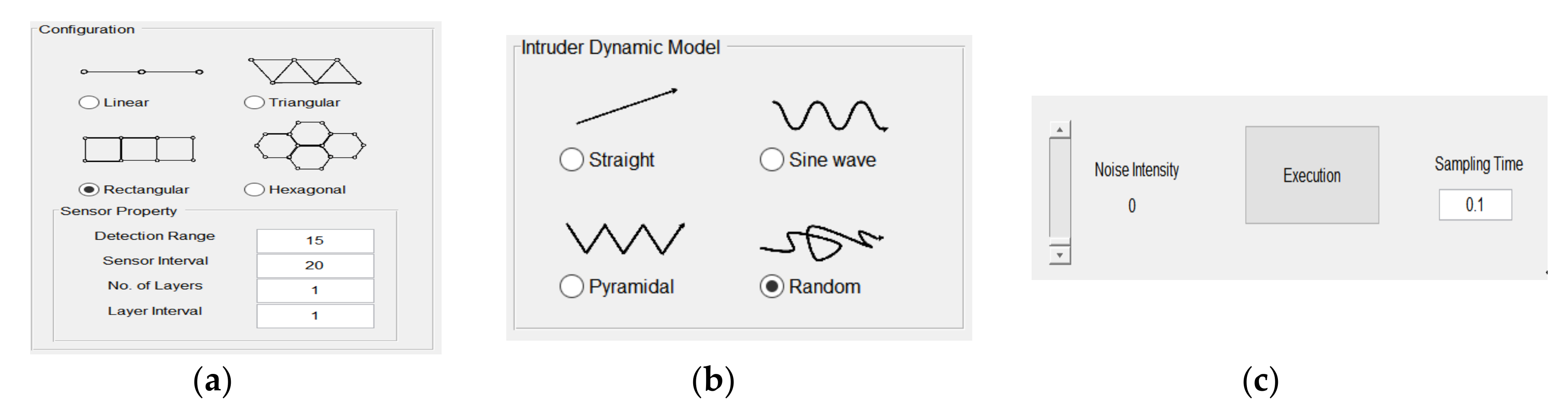
4.1.1. Sensor Configuration

The sensor configuration in Figure 5a comprises a domain where selection of the sensor structure is enabled and a sensor property domain controls its detailed content. The sensor structure includes linear, triangular, rectangular, and hexagonal forms, and one of these is selected. Selection of the sensor structure is followed by setting the detection radius of the sensor the user desires, the interval between the sensors, and the number of layers in which the sensors are arranged; these are set by the user through the sensor properties.

4.1.2. The Intruder Behavior Model

The intruder behavior model, shown in Figure 5b, is a domain where the type of behavior model is established. It consists of a straight model (a model of constant velocity), sine wave and pyramidal models (models of constant acceleration), and a random model with random movement.

4.1.3. Other Issues

Figure 5c shows a noise intensity domain where the size of the covariance of the noise components is set, and a sampling time domain where the time intervals are set. The size of the covariance, which is a slide bar of the noise intensity, is set using a mouse. The sampling time is set by the user, who fills in the value.

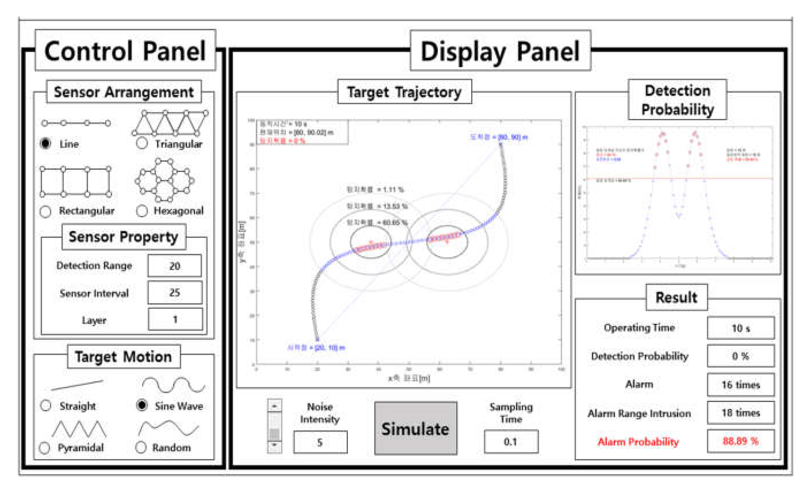
4.2. Display Domain

The display panel shown in Figure 6 is a domain where a simulation can be viewed with images under the method established in the control panel. The simulation provides information that is updated on a real time basis and the condition of the current progress may be observed, enabling real-time surveillance. The user can identify its performance with the simulation result values according to the set environment through graphs and numerical values.

4.3. Performance Evaluation and Results

For the intruder behavior model, the sampling interval T at 0.1 s, the measured noise intensity $q_{cv}$, $q_{ca}$ at $5 m^2/{\sec }^4$, the covariance matrix of the measured values at $R_i(k)$, the initial values of the state error covariance matrix for an intruder behavior model of constant velocity and acceleration $P_{cv}(0)$ and $P_{ca}(0)$ were set as follows.

$$R_i(k)=\left[\begin{array}{cc}{5}^2& 0\\ 0& 5^2\end{array}\right]m^2,$$

(24)

$$P_{cv}(0)={10}^{2}I(4\times 4)m^2, P_{ca}(0)={10}^{2}I(6\times 6)m^2.$$

(25)

In addition, the intruder behavior model is set with the movement of a sine wave that moves from the starting point at (20,10) m to the end point at (80,90) m.

The performance of the sensors in the sensor arrangement is evaluated with 12 scenarios, using two sensors at intervals of 15, 20, and 25 m and sensor detection radiuses at 20, 25, and 30 m. For the detection probability of the overlapped detection domain, the variance of Equation (22) of the sensor fusion technology algorithm is set at ${\sigma }_1{}^2={\sigma }_2{}^2$, and the standard for sounding the alarm is set at a detection probability of 60.65% or more.

The performance evaluation was conducted using the result value calculated through 100 Monte Carlo simulations under the same condition.

In addition, the intruder behavior model is set with the movement of a sine wave that moves from the starting point at (10,20) m to the end point at (80,90) m.

The performance of the sensors in the sensor arrangement is evaluated with 12 scenarios, using two sensors at intervals of 15, 20, and 25 m and sensor detection radiuses at 20, 25, and 30 m. For the detection probability of the overlapped detection domain, the variance of Equation (22) of the sensor fusion technology algorithm is set at ${\sigma }_1{}^2={\sigma }_2{}^2$, and the standard for sounding the alarm is set at a detection probability of 60.65% or more.

The performance evaluation was conducted using the result value calculated through 100 Monte Carlo simulations under the same condition.

Table 1. Performance comparison of the various sensor interval and detection radius.

Detection Radius	Sensor Interval = 15 m
	Alarm	Intrusion Alarm Domain	Intrusion Detection Domain
20 m	1155 times	1400 times	3900 times
25 m	1116 times	1400 times	4300 times
30 m	1002 times	1255 times	4700 times
Detection Radius	Sensor interval = 20 m
	Alarm	Intrusion alarm domain	Intrusion detection domain
20 m	1674 times	2040 times	4900 times
25 m	1579 times	1800 times	5300 times
30 m	1522 times	1800 times	5700 times
Detection Radius	Sensor interval = 25 m
	Alarm	Intrusion alarm domain	Intrusion detection domain
20 m	2269 times	2700 times	5904 times
25 m	2187 times	2600 times	6500 times
30 m	2033 times	2600 times	6706 times

shows that a narrower interval between the sensors or a greater detection radius increased the number of instances of intrusion into the alarm domain. In other words, the performance in terms of finding intruders was improved. Nonetheless, in the case where the interval between the sensors were 25 and 30 m and the detection radii of the sensors were 20 and 25 m, the number of intrusions into the alarm domain did not change. This was considered a problem with the sampling time interval; therefore, an additional performance evaluation according to the sampling time was also performed.

Table 2. Comparison of performance according to sampling time in 25 m sensor interval.

Detection Radius	Sampling Time = 0.01 s
	Alarm	Intrusion Alarm Domain	Intrusion Detection Domain
20 m	20,781 times	21,700 times	20,318 times
25 m	24,900 times	26,200 times	24,800 times
30 m	59,900 times	64,300 times	67,900 times
Detection Radius	Sampling time = 0.05 s
	Alarm	Intrusion alarm domain	Intrusion detection domain
20 m	4550 times	5300 times	11,900 times
25 m	4348 times	5200 times	12,900 times
30 m	4084 times	5000 times	13,500 times
Detection Radius	Sampling time = 0.1 s
	Alarm	Intrusion alarm domain	Intrusion detection domain
20 m	2269 times	2700 times	5904 times
25 m	2187 times	2600 times	6500 times
30 m	2033 times	2600 times	6706 times

shows that when the sampling time is changed from 0.1 s (the first assumed sampling time) to 0.05 s and to 0.01 s, changes in response to the detection radius are observed in Table 2 that did not occur in Table 1. In other words, for detailed measurements, the sampling time should be set short. Nonetheless, shortening of the sampling time interval results in accumulation of a lot of information, but the obtained information becomes imprecise, resulting in increased operation time. In other words, the user should establish an appropriate size for the sampling time that considers the measurement environment.

5. Conclusions and Future Plans

This paper dealt with the development of a simulator for an underwater aquaculture facility surveillance system. The simulator enables a performance evaluation of an alarm through a computer program prior to the establishment of the actual surveillance system. A reliable simulator measurement result was obtained by two methods. First, an intruder behavior model was expressed into a state space equation that can control several variables at the same time to express various movements of intruders. A sensor model was then designed with a statistical approach to deal with the decreased detection performance that occurs for diverse reasons when detecting objects with sensors; Matlab GUI was used as a simulator. The resulting system allows diverse experimental environments to be set simply by the arrangement of the sensors and the detection radius of the sensors, thereby enabling comparative analysis of performance of underwater surveillance systems under different experimental environments.

Nonetheless, this study did not examine the actual perception of intruders, although a high possibility of malfunctions could occur in an ocean environment where diverse variables exist. Moreover, the user should establish an appropriate size for the sampling time, due to accumulation of a lot of information the obtained information becomes imprecise, resulting in increased operation time. In particular, when intruders appear in the underwater surveillance system, they have different positions; therefore, meeting the conditions for perceiving intruders will be challenging. Thus, formulating an algorithm for intruder perception should be addressed in future studies that identify the appropriate characteristic conditions for perceiving intruders.

References

- Kim, C.-S.; Jeong, J.-S.; Park, S.-H. A study on remote monitoring system for protecting aquaculture farms. J. Korean Soc. Mar. Environ. Saf. 2004, 10, 55–60. (In Korean) [Google Scholar]
- Yim, J.B.; Nam, T.K. Implementation of unmanned aquaculture security system. J. Korean Soc. Mar. Environ. Saf. 2007, 13, 61–67. (In Korean) [Google Scholar]
- Reshma, B.; Kumar, S.S. Precision aquaculture drone algorithm for delivery in sea cages. In Proceedings of the 2016 IEEE International Conference on Engineering and Technology, Coimbatore, India, 17–18 March 2016; pp. 1264–1270. (In India). [Google Scholar]
- Akyildiz, I.; Su, W.; Sankarasubramaniam, Y.; Cayirci, E. A survey on sensor networks. IEEE Commun. Mag. 2002, 40, 102–114. [Google Scholar] [CrossRef] [Green Version]
- Akyildiz, I.; Su, W.; Sankarasubramaniam, Y.; Cayirci, E. Wireless sensor networks: A survey. Comput. Netw. 2002, 38, 393–422. [Google Scholar] [CrossRef] [Green Version]
- Min, S.H.; Choi, J.W. Development of an underwater fish farm surveillance simulator. Inst. Control Robot. Syst. 2017, 23, 497–502. [Google Scholar] [CrossRef]
- Yu, C.H.; Choi, J.W. Underwater wireless sensor networks-based distributed tracking filter for a fish farm trespasser. J. Inst. Control Robot. Syst. 2018, 24, 133–140. [Google Scholar] [CrossRef]
- Yu, C.H.; Choi, J.W. Interacting multiple model filter-based distributed target tracking algorithm in underwater wireless sensor networks. Int. J. Control Autom. Syst. 2014, 12, 618–627. [Google Scholar] [CrossRef]
- Samuel, K.; Choi, J.W. Improved IMM filter for tracking a highly maneuvering target with mixed system noises. Int. J. Control Autom. Syst. 2018, 16, 2763–2771. [Google Scholar] [CrossRef]
- Park, C.R.; Bae, M.S. Current state of open sea aquaculture and promotion work for vitalization. Nat. Assem. Res. Serv. Field Surv. Rep. 2012, 23, 1–12. (In Korean) [Google Scholar]
- Li, X.R.; Jilkov, V.P. Survey of maneuvering target tracking. Part I: Dynamic models. IEEE Trans. Aerosp. Electron. Syst. 1998, 34, 103–123. [Google Scholar]
- Bar-Shalom, Y.; Li, X.R.; Kirubarajan, T. Estimation with Applications to Tracking and Navigation: Theory, Algorithms, and Software; John Wiley & Sons, Inc.: Hoboken, NJ, USA, 2001. [Google Scholar]
- Gelb, A.; Kasper, J.F.; Nash, R.A.; Price, C.F.; Sutherland, A.A. Applied Optimal Estimation; The Massachusetts Institute of Technology Press: Cambridge, MA, USA, 1974. [Google Scholar]
- Maybeck, P.S. Stochastic Models, Estimation, and Control; Academic Press: Cambridge, MA, USA, 1994; Volume 1. [Google Scholar]
Figure 1.
Co-culture of abalone and sea cucumber: (a) floating cages for abalone production and sea cucumber; (b) sea cucumber cultivation cages at the bottom.
Figure 2.
The components of a sea cucumber aquaculture facility: (a) utility farming unit; (b) cultivation cage.
Figure 3.
Detection performance improvement resulting from sensor fusion.
Figure 4.
An integrated simulator for a Matlab GUI-based underwater aquaculture surveillance system.
Figure 5.
The control panel: (a) sensor configuration, (b) intruder behavior models, (c) noise intensity and sampling time.
Figure 6.
Display screen for control panel.