A Bayesian Approach to Heavy-Tailed Finite Mixture Autoregressive Models

Abstract

In this paper, a Bayesian analysis of finite mixture autoregressive (MAR) models based on the assumption of scale mixtures of skew-normal (SMSN) innovations (called SMSN–MAR) is considered. This model is not simultaneously sensitive to outliers, as the celebrated SMSN distributions, because the proposed MAR model covers the lightly/heavily-tailed symmetric and asymmetric innovations. This model allows us to have robust inferences on some non-linear time series with skewness and heavy tails. Classical inferences about the mixture models have some problematic issues that can be solved using Bayesian approaches. The stochastic representation of the SMSN family allows us to develop a Bayesian analysis considering the informative prior distributions in the proposed model. Some simulations and real data are also presented to illustrate the usefulness of the proposed models.

1. Introduction

Data analysts apply computational models to describe and infer statements about complex datasets. Mixture models are a valuable class of these models. Finite mixture models are of great importance in statistical inferences. The multimodality, skewness, kurtosis, and unobserved heterogeneity are usually observed in many datasets, for example time series datasets. Importance of mixture distributions, which are the main tools for statistical mixture models, has been noted by many references [1,2,3,4,5,6,7,8]. Various statistical fields containing time series modeling and regression analysis frequently use the mixture modeling. In fact, in analyzing time series data, some events may affect and change the behavior of data over time, for example, finance crises in many financial or panel time series datasets. The finite mixture autoregressive (MAR) models were suggested by Wong and Li [7], to catch the multimodal phenomena, are flexible and applicable in many fields, such as electroencephalogram modeling in medicine [8], interest rates and bond pricing [9], Forex rate [10], and other various fields such as telecommunications, hydrology, biology, sociology, and medical sciences.

Most researchers considered the MAR models based on Gaussian distribution, which are called Gaussian mixture of autoregressive (GMAR) models [7,8,9,10,11]. The GMAR models are sensitive to the existence of outliers, heavy tailed distribution and asymmetry in datasets, and thus some authors considered MAR models based on non-Gaussian, heavy tailed and/or asymmetric distributions. Wong and Li [12] introduced logistic mixture autoregressive model. Wong and Chan [13] also introduced a student t–mixture autoregressive model and discussed its inferences and then applied this model to the heavy tailed financial data.

The SMSN family, introduced by Branco [1], is a rich family containing famous symmetric scale mixtures of normal (SMN; [14]) distributions and asymmetric distributions such as the skew-t, skew-slash and skew-contaminated-normal distribution. The MAR model based on the SMSN innovations, hereafter called SMSN–MAR models, has reasonable performance to model real time series data with outliers and skewness. The various MAR model members can determine weights to each observation, and therefore each single observation affects the estimation of the model’s parameters, and it leads to robust inferences. Bayesian inferences of the MAR models have some advantages compared to classical methods, that some of them are discussed below.

For maximum likelihood computations and classical inference of a MAR model, although the numerical optimization algorithms such as the EM–algorithm can be applied, converging to the major mode may fail, while this is not an issue in Bayesian inferences. Furthermore, in the MAR models there exist many situations with indirect information about the parameters or large changes in the results by small changes in the data. When we consider a sample from a MAR model, the sample includes no information about the parameters of one or more components with a positive probability. Therefore, the likelihood function can be unbounded and consequently the resultant likelihood estimates are only local maximum. Using suitable priors and some Bayesian techniques can solve such problems. Another problematic issue on the classical likelihood–based inference is that, in MAR model, the component parameters are not identifiable marginally, so distinguishing any component from other components in the likelihood is hard. The identifiability is not an important problem in Bayesian inferences. Some of the other advantages of the Bayesian inferences of the mixture models are given in [15,16].

In this paper, we consider a Bayesian technique to find estimates of the SMSN–MAR models by the Gibb sampling scheme and application of the Markov Chain Monte Carlo (MCMC) methods. The main characteristics of the SMSN distributions are reviewed in Section 2. In Section 3, we consider the MAR models and apply the Bayesian methodology for estimating the proposed MAR model’s parameters. To evaluate the Bayesian estimates of parameters and performance of the proposed model, numerical studies and a real practical example are reported in Section 4. The conclusion is provided in the last section.

2. The SMSN Distributions

A random variable $Y$ is belonged to the scale mixtures of skew normal (SMSN) family, if it has the following representation:

$$Y=\mu +k^{1/2}\left(U\right)Z,$$

(1)

where the random variable $Z$ follows a skew-normal distribution in [17], where ${\sigma }^2$ and $\lambda$ are respectively scale and skewness parameters, the function $k\left(u\right)$ is positive respect to $u$, $U$ is the scale random variable with density function or pmf $h\left(\cdot ;\mathit{\nu }\right)$ and distribution function $H\left(\cdot ;\mathit{\nu }\right)$, and the vector or scalar $\mathit{\nu }$ indexes the distribution of $U$. The random variable $Y$ is denoted by $Y ~ SMSN\left(\mu ,{\sigma }^2,\lambda ,\mathit{\nu }\right)$, and in this work, because of its suitable mathematical properties, we let $k\left(u\right)=1/u$, so $Y|U=u~SN\left(\mu ,u^{-1}{\sigma }^2,\lambda \right)$. Therefore, the density of$Y$is given by

$$f\left(y;\mathit{\theta }\right)=2{{\displaystyle \int }}_0^{\infty }\varphi \left(y;\mu ,u^{-1}{\sigma }^2\right)\mathsf{\Phi }\left(\frac{u^{1/2}\lambda \left(y-\mu \right)}{\sigma }\right)dH\left(u|\mathit{\nu }\right),$$

(2)

where$\mathit{\theta }={\left(\mu ,{\sigma }^2,\lambda ,{\mathit{\nu }}^{\top }\right)}^{\top }$, and $\varphi (\cdot )$ and$\mathsf{\Phi }(\cdot )$ are density and distribution functions of the standard normal distribution, respectively.

Proposition 1.

Let $Y ~ SMSN\left(\mu ,{\sigma }^2,\lambda ;H\right)$,

(a)

If $E\left[U^{-1/2}\right]<\infty$, then ${\mu }_Y=E\left[Y\right]=\mu -b\Delta$,

(b)

If $E\left[U^{-1}\right]<\infty$, then ${\sigma }_Y^2=Var\left[Y\right]={\sigma }^2{k}_2-b^2{\Delta }^2$,

(c)

$Y$ has a stochastic representation given by$Y=\mu +\Delta W+\gamma U^{-1/2}{W}_1,$

where$b=-\sqrt{2/\pi }E\left[U^{-1/2}\right]$, $\delta =\lambda /\sqrt{1+{\lambda }^2}$, $\Delta =\sigma \delta$, ${\gamma }^2={\sigma }^2-{\Delta }^2$, $W=U^{-1/2}\left|w_0\right|$, and $W_0$ and $W_1$ are independent standard normal random variables.

The famous members of the SMSN family are the scale mixtures of normal (SMN) family [8,13], as the symmetric members of the SMSN family, and skew-normal (SN), skew-t (ST), skew-slash (SSL) and skew-contaminated-normal (SCN) distributions. More details are given in [18,19].

3. The SMSN–MAR Model and Bayesian Estimates

3.1. The SMSN–MAR Model

In this paper, we study the MAR model, which has been studied by Wong and Li [7], and Wong and Chan [20], due to its flexibility in use for non-linear time series analysis. This model is represented by

$$\begin{array}{c}{X}_t={\phi }_{i,0}+{{\displaystyle \sum }}_{j=1}^{p_i}{\phi }_{i,j}{X}_{t-j}+{\epsilon }_{i,t}, \mathrm{with} \mathrm{probability} {\pi }_i; i=1,2,\dots ,\mathrm{g}; t\\ =0,\pm 1,\pm 2,\dots ,\end{array}$$

(3)

or equivalently,

$$X_t=\{\begin{array}{c}{\phi }_{1,0}+{{\displaystyle \sum }}_{j=1}^{p_1}{\phi }_{1,j}{X}_{t-j}+{\epsilon }_{1,t}; \mathrm{with} \mathrm{probability} {\pi }_1\hfill \\ {\phi }_{2,0}+{{\displaystyle \sum }}_{j=1}^{p_2}{\phi }_{2,j}{X}_{t-j}+{\epsilon }_{2,t}; \mathrm{with} \mathrm{probability} {\pi }_2, t=0,\pm 1,\pm 2,\dots ,\hfill \\ ⋮\\ {\phi }_{\mathrm{g},0}+{{\displaystyle \sum }}_{j=1}^{p_{\mathrm{g}}}{\phi }_{\mathrm{g},j}{X}_{t-j}+{\epsilon }_{\mathrm{g},t}; \mathrm{with} \mathrm{probability} {\pi }_{\mathrm{g}}\hfill \end{array}$$

where

• g is a known positive integer which indicates the number of components in the model;
• each component occurs with probabilities${\pi }_i>0, i=1,\dots ,\mathrm{g}, {{\displaystyle \sum }}_{i=1}^{\mathrm{g}}{\pi }_i=1,$ which obeys a discrete distribution $\mathit{\pi }$;
• for each $i=1,\dots ,\mathrm{g}$,

  ➢

  the ith autoregressive component is of order $p_i\ge 1$;

  ➢

  ${\phi }_{i,j}, j=0,\dots ,p_i$, are the autoregressive coefficients of the ith components;

  ➢

  each ith innovation’s component${\epsilon }_{i,t}$ distributed as following:

  $${\epsilon }_{i,t} {\begin{array}{c}\begin{array}{c} \\ i.i.d.\end{array}\\ ~\\ \end{array}}^{ } SMSN\left(b_i{\Delta }_i, {\sigma }_i^2, {\lambda }_i, {\mathit{\nu }}_i\right); i=1,\dots ,\mathrm{g}; t=0,\pm 1,\pm 2,\dots$$

  (4)

  where $b_i=-\sqrt{2/\pi }E\left[U_i^{-r/2}\right]$, ${\delta }_i={\lambda }_i/\sqrt{1+{\lambda }_i^2}$, ${\Delta }_i={\sigma }_i{\delta }_i$ and ${\gamma }_i^2={\sigma }_i^2+{\Delta }_i^2$. Also in each ith component, $\left\{{\epsilon }_{i,t}\right\}$ are jointly independent and are independent of past $X_t$s and also independent of other component’s innovations.

Hereafter, this model will be called SMSN–MAR(p,g). Note that in each component, when$b_i$ exists,$E\left({\epsilon }_{i,t}\right)=0,$ and$\mathrm{Var}\left({\epsilon }_{i,t}\right)={\sigma }_i^2{k}_{i2}-b_i^2{\Delta }_i^2 ; i=1,\dots ,\mathrm{g}$. Note that we can assume that the vector of coefficients in MAR models, distributed as$\mathit{\pi }$, therefore, this model can be also interpreted as random coefficients autoregressive (RCA) model.

Without loss of generality, it is convenient to set $p={\max }_{i=1,\dots ,\mathrm{g}} p_i$ and${\phi }_{i,j}=\dots ={\phi }_{i,p}=0$ for$j>p_i$. Also, let$\left\{Z_t\right\}$ be an i.i.d. sequence of random variables which are distributed as$\mathit{\pi }$ (Multinomial), such that$P\left(Z_t=i\right)={\pi }_i,i=1,\dots ,\mathrm{g}$, that determines the components, and be independent of innovations and random history of model$\mathit{X}={\left(X_1,\dots ,X_n\right)}^{\top }$. Therefore, $X_t$obeys from ith component of MAR model, if$Z_t=i$. Thus, Equation (3) can be written as

$$X_t={\phi }_{Z_t,0}+{{\displaystyle \sum }}_{j=1}^p{\phi }_{Z_t,j}{X}_{t-j}+{\epsilon }_{Z_t,t}, t=0,\pm 1,\pm 2,\dots$$

(5)

where$Z_t~ \mathrm{Multinomial}\left(1,{\pi }_i,\dots ,{\pi }_{\mathrm{g}}\right)$.

It is convenient to set vector and matrix notations of sample$\mathit{X}={\left(X_1,\dots ,X_n\right)}^{\top }$ in the form of ${\mathit{X}}_{t-1}={\left(1,X_{t-1},\dots ,X_{t-p}\right)}^{\top };t=1,\dots ,n$,${\mathit{\varphi }}_{Z_t}={\left({\phi }_{0,Z_t},\dots ,{\phi }_{p,Z_t}\right)}^{\top }$, ${\mathit{\epsilon }}_{Z_t}={\left({\epsilon }_{Z_t,1},\dots ,{\epsilon }_{Z_t,n}\right)}^{\top }$ and $\mathit{A}$ be the $n\times p$ matrix whose tth row is ${\mathit{X}}_{t-1}$, in the rest of the paper. Thus, the following matrix representation

$$\mathit{X}=\mathit{A}{\mathit{\varphi }}_{Z_t}+{\mathit{\epsilon }}_{Z_t},$$

(6)

Note that in Equation (7), $X_t={\mathit{\varphi }}_{Z_t}^{\top }{\mathit{X}}_{t-1}+{\epsilon }_{Z_t,t}$ where $Z_t, t=1,\dots ,\mathrm{g}$ and distributed as$\mathit{\pi }$, so by Equation (5) we have

$$X_t|{\mathit{X}}_{t-1},Z_t~SMSN\left({\mathit{\varphi }}_{Z_t}^{\top }{\mathit{X}}_{t-1}+b_{Z_t}{\Delta }_{Z_t}, {\sigma }_{Z_t}^2, {\lambda }_{Z_t}, {\mathit{\nu }}_{Z_t}\right); Z_t=1,\dots ,\mathrm{g}, t=1,\dots ,n.$$

(7)

Therefore, the density of $N_t$ is given by

$$f_{X_t|X_{t-1},\dots , X_{t-p}}\left(x_t;\mathit{\theta }\right)={{\displaystyle \sum }}_{i=1}^{\mathrm{g}}{\pi }_i{f}_i\left(x_t|{\mathit{X}}_{t-1},{\mathit{\theta }}_i\right),$$

(8)

where $f_i\left(.|{\mathit{X}}_{t-1},{\mathit{\theta }}_i\right)$ is the pdf of $SMSN\left({\mathit{\varphi }}_i^{\top }{\mathit{X}}_{t-1}+b_i{\Delta }_i, {\sigma }_i^2, {\lambda }_i, {\mathit{\nu }}_i\right)$ defined in Equation (2), hereafter note that $\mathit{\theta }={\left({\mathit{\theta }}_1^{\top },\dots ,{\mathit{\theta }}_{\mathrm{g}}^{\top }\right)}^{\top }$, where${\mathit{\theta }}_i={\left({\pi }_i,{\mathit{\varphi }}_i^{\top },{\sigma }_i^2,{\lambda }_i,{\mathit{\nu }}_i^{\top }\right)}^{\top },i=1,\dots ,\mathrm{g}$ be the vector of parameters.

By using Markovian property of this model, we have that$L\left(\mathit{\theta }|\mathit{X}\right)=f_X\left(X_1, \dots , X_n;\mathit{\theta }\right)=$ ${{\displaystyle \prod }}_{t=1}^n{f}_{X_t|X_{t-p},\dots , X_{t-1}}\left(X_t;\mathit{\theta }\right)$, where$f_X(.)$ be the density of$\mathit{X}$. An auxiliary determiner of components in MAR models (6), can be expressed in the random vector ${\mathit{Z}}_t={\left(Z_{t1},\dots ,Z_{t\mathrm{g}}\right)}^{⊺}$, where

$$Z_{ti}=\{\begin{array}{l}1,\mathrm{if}t\mathrm{th}\mathrm{observation}\mathrm{of}\mathrm{MAR}\mathrm{process}\mathrm{obeys}\mathrm{the}i\mathrm{th}\mathrm{compoment}\\ 0,\text{otherwise}\end{array}$$

Therefore, under the above approach, the latent random vector ${\mathit{Z}}_t,t=1,\dots ,n$ has the following multinomial ${\mathit{Z}}_t ~Multinomial\left(1,{\pi }_1,\dots ,{\pi }_{\mathrm{g}}\right)$ with the following probability mass function:

$$\mathrm{P}\left(Z_i=z_i\right)={\pi }_1^{z_{t1}}{\pi }_2^{z_{t2}}\dots {\pi }_{\mathrm{g}}^{z_{t\mathrm{g}}};t=1,\dots ,n,$$

such that ${\Sigma }_{i=1}^g{\pi }_i=1$, ${\mathsf{\pi }}_i>0,i=1,\dots ,\mathrm{g}$. Therefore,

$$X_t|{\mathit{X}}_{t-1},Z_{ti}=1~SMSN\left({\mathit{\varphi }}_i^{\top }{\mathit{X}}_{t-1}+b_i{\Delta }_i, {\sigma }_i^2, {\lambda }_i, {\mathit{\nu }}_i\right), i=1,\dots ,\mathrm{g}; t=1,\dots ,n.$$

Also, to provide a MCMC method, we have:

$$X_t|{\mathit{X}}_{t-1},W_{ti}=w_{ti},U_{ti}=u_{ti},Z_{ti}=1 ~N\left({\mathit{\varphi }}_i^{\top }{\mathit{X}}_{t-1}+{\Delta }_i{w}_{ti}, u_{ti}^{-1}{\gamma }_i^2 \right),$$

$$W_{ti}|U_{ti}=u_{ti},Z_{ti}=1 ~ T{N}_1\left(b_i, u_{ti}^{-1}\right)I_{\left(b_i,\infty \right)},$$

$$U_{ti}|Z_{ti}=1 ~ H\left(u_{ti}; {\mathit{\nu }}_i\right),$$

$${\mathit{Z}}_t ~Multinomial\left(1,{\pi }_1,\dots ,{\pi }_{\mathrm{g}}\right),$$

for $t=1,\dots ,n$. Let $\mathit{D}={\left({\mathit{X}}^{\top },{\mathit{M}}^{\top }\right)}^{\top }$ as the complete data, where$\mathit{X}$ is the observed part of data, ${\mathit{M}}^{\top }=$ ${\left({\left(W_{ti},U_{ti},Z_{ti}\right)}_{t=1}^n\right)}_{i=1}^{\mathrm{g}}$ is the missing parts of data, and $\mathit{\theta }$ is the vector of unknown parameters. The conditional likelihood function based on the complete data is provided by

$$L\left(\mathit{\theta }|\mathit{D}\right)={{\displaystyle \prod }}_{t=1}^n{{\displaystyle \prod }}_{i=1}^{\mathrm{g}}{\left({\pi }_i{f}_{X_t|{\mathit{X}}_{t-1},W_{ti},U_{ti},Z_{ti}}\left(X_t;{\mathit{\theta }}_i\right)f_{W_{ti}|U_{ti},Z_{ti}}\left(W_{ti};{\mathit{\theta }}_i\right)f_{U_{ti}|Z_{ti}}\left(U_{ti};{\mathit{\theta }}_i\right)\right)}^{Z_{ti}}.$$

3.2. Bayesian Approach

In this part, we use the Bayesian approach by applying MCMC algorithms for the model in Equation (3). We consider informative priors under squared error loss function (SEL). To consider the prior distributions for the parameters of the considered model, we assign prior distributions to the parameters as follow:

$$\begin{gathered} {\mathit{\varphi }}_i ~ N_{p+1}\left({\mathit{\phi }}_i, {\mathsf{\Sigma }}_i\right), {\Delta }_i~ N\left({\mu }_{\Delta i},{\sigma }_{\Delta i}^2\right), {\gamma }_i^2 ~ \mathrm{IG}\left({\rho }_i/2,{\varrho }_i/2\right), \\ \mathit{\pi }=\left({\pi }_1,\dots ,{\pi }_{\mathrm{g}}\right) ~ \mathrm{Dir}\left({\delta }_1,\dots ,{\delta }_{\mathrm{g}}\right), \end{gathered}$$

(9)

for $i=1,\dots ,\mathrm{g},$ where $\mathrm{Dir}$ and IG denote the Dirichlet distribution and the Inverse-Gamma distribution, respectively.

The prior distribution assigned to ${\mathit{\nu }}_i, i=1,\dots \mathrm{g}$, varies with the particular SMSN distributions. For skew–t model, we can consider ${\nu }_i~\exp \left({\mathsf{\varsigma }}_i/2\right)I_{\left(2,\infty \right)},$ exponential distribution with mean$2/{\mathsf{\varsigma }}_i$ before truncation, for skew–slash model, we can consider ${\nu }_i~\mathrm{Gamma}\left(a_i,b_i\right)$ with small positive values $a_i$ and $b_i$ such that $b_i\ll a_i$, and for skew–contaminated–normal model, the independent and non-informative $U\left(0,1\right)$prior distributions are considered for each component of ${\mathit{\nu }}_i={\left({\nu }_i,{\gamma }_i\right)}^{\top }$. We also assume that priors are independent and all hyper-parameters (parameters of priors) are known, which guarantees that all posteriors are proper. The joint posterior of $\mathit{\theta }$ and missing variables is in the form of $\pi \left(\mathit{\theta }|\mathit{D}\right)\propto L\left(\mathit{\theta }|\mathit{D}\right)\pi \left(\mathit{\theta }\right)$, which is not analytically tractable, but the MCMC methods such as the Gibbs sampling, will be applied to draw samples from the marginal of conditional posteriors which are shown as follows, when ${\mathit{\theta }}_{\left(-m\right)}$, means the mth element of $\mathit{\theta }$ has been removed (Algorithm 1).

Algorithm 1: MCMC

For$i=1,\dots ,\mathrm{g}$, and$t=1,\dots ,n$, ${\mathit{Z}}_t|\mathit{\theta }, \mathit{U},\mathit{W};\mathit{X}~Multinomial\left(1,p_1,\dots ,p_{\mathrm{g}}\right),$ $\mathit{\pi }|{\mathit{\theta }}_{\left(-\pi \right)}, \mathit{D}~Dir\left({\delta }_1+{{\displaystyle \sum }}_{t=1}^n{Z}_{t1},\dots ,{\delta }_{\mathrm{g}}+{{\displaystyle \sum }}_{t=1}^n{Z}_{t\mathrm{g}}\right)$, $W_{ti}|\mathit{\theta }, \mathit{U},Z_{ti}=1;\mathit{X}~T{N}_1\left({\mu }_{W_{ti}}+b_i,u_{ti}^{-1}{M}_i^2\right)I_{\left(b_i,\infty \right)},$ ${\mathit{\varphi }}_i|{\mathit{\theta }}_{\left(-{\mathit{\varphi }}_i\right)},Z_{ti}=1,\mathit{D}~N_{p+1}\left({\mathit{\mu }}_{{\mathit{\varphi }}_i}, {\mathsf{\Sigma }}_{{\mathit{\varphi }}_i}\right),$ ${\gamma }_i^2|{\mathit{\theta }}_{\left(-{\gamma }_i\right)}, Z_{ti}=1,\mathit{D}~IG\left({\rho }_i,{\tau }_i\right),$ ${\Delta }_i|{\mathit{\theta }}_{\left(-{\Delta }_i\right)},Z_{ti}=1, \mathit{D}~N\left(\frac{{\beta }_i{\sigma }_{\Delta i}^2+{\gamma }_i^2{\mu }_{\Delta i}}{{\alpha }_i{\sigma }_{\Delta i}^2+{\gamma }_i^2},\frac{{\alpha }_i{\sigma }_{\Delta i}^2+{\gamma }_i^2}{{\gamma }_i^2{\sigma }_{\Delta i}^2}\right),$ $U_{ti}|\mathit{\theta },Z_{ti}=1,\mathit{D}~H_{post}\left(u;\mathit{\theta },\mathit{\nu }\right),$ $\mathit{\nu }|{\mathit{\theta }}_{\left(-\nu \right)},\mathit{U},Z_{ti}=1,\mathit{D}~f_{post}\left(\mathit{\nu } ;\mathit{\theta }\right),$ where${\mathit{Z}}_t={\left(Z_{t1},\dots ,Z_{t\mathrm{g}}\right)}^{\top }$,$p_i=\frac{{\pi }_{i}f\left(X_t|{\mathit{X}}_{t-1};{\mathit{\theta }}_i\right)}{{{\displaystyle \sum }}_{i=1}^{\mathrm{g}}{\pi }_{i}f\left(X_t|{\mathit{X}}_{t-1};{\mathit{\theta }}_i\right)}$,$M_i^2=\frac{{\gamma }_i^2}{{\gamma }_i^2+{\Delta }_i^2}$, ${\mu }_{W_{ti}}=M_i^2\frac{{\Delta }_i}{r_i^2}(X_t-{\mathit{\varphi }}_i^{⊺}{\mathit{X}}_{t-1}-b_i{\Delta }_i)$ ,${\mathit{\mu }}_{{\mathit{\varphi }}_i}={\left({\gamma }_i^{-2}\left({\mathit{Z}}^{\top }{\mathit{\Lambda }}_i\mathit{Z}\right)+{\mathit{M}}_{i0}^{-1}\right)}^{-1}\left({\gamma }_i^{-2}\left({\mathit{Z}}^{\top }{\mathit{\Lambda }}_i\mathit{Z}\right){\mathit{M}}_i+{\mathit{M}}_{i0}^{-1}{\mathit{\varphi }}_{i0}\right)$,${\mathsf{\Sigma }}_{{\mathit{\varphi }}_i}={\left({\gamma }_i^{-2}\left({\mathit{Z}}^{\top }{\mathit{\Lambda }}_i\mathit{Z}\right)+{\mathit{M}}_{i0}^{-1}\right)}^{-1}$, ${\rho }_i=\frac{n-p+p_i+\mathrm{i}}{2}$,${\tau }_i=\frac{1}{2}\left({\varrho }_i+{\left({\mathit{\varphi }}_i-{\mathit{M}}_i\right)}^{\top }\left({\mathit{Z}}^{\top }{\mathit{\Lambda }}_i\mathit{Z}\right)\left({\mathit{\varphi }}_i-{\mathit{M}}_i\right)\right)$,${\alpha }_i={\mathit{W}}_i^{\top }{\mathit{\Lambda }}_i \mathit{W}$and${\beta }_i={\mathit{W}}_i^{\top }{\mathit{\Lambda }}_i\left(X_t-{\mathit{\varphi }}_i^{⊺}{\mathit{X}}_{t-1}-b_i{\Delta }_i\right)$.

Finally, in order to complete the specifications of the sampling via MCMC methods, the posterior distribution of the latent variable $U_{ti},t=1,\dots ,n, i=1,\dots ,\mathrm{g}$, $H_{post}\left(u;\mathit{\theta },\mathit{\nu }\right)$, and its indexed parameter${\mathit{\nu }}_i$, ${\mathrm{f}}_{post}\left(\mathit{\nu };\mathit{\theta }\right)$, should be determined. Set $c_{ti}={\left(X_t-{\mathit{\varphi }}_i^{\top }{\mathit{X}}_{t-1}-{\Delta }_i{W}_{ti}\right)}^2/{\sigma }_i^2+{\left(W_{ti}-b_i\right)}^2$, we then have, for $t=–1,\dots ,n$ and the several models given as:

∎

ST–MAR:

$$U_{ti}|\mathit{\theta },Z_{ti}=1,\mathit{D}~\mathrm{Gamma}\left(\frac{{\nu }_i+2}{2},\frac{{\nu }_i+c_{ti}}{2}\right), i=1,\dots ,\mathrm{g}, t=1,\dots ,n,$$

(10)

and

$$\begin{array}{cc}\hfill \pi \left({\nu }_i|{\mathit{\theta }}_{\left(-{\nu }_i\right)},Z_{ti}=1,\mathit{D}\right)& \propto {\left(2^{{\nu }_i/2}\mathsf{\Gamma }\left({\nu }_i/2\right)\right)}^{-n}\hfill \\ & \times \mathrm{Gamma}\left(\frac{n{\nu }_i}{2}-1,\frac{1}{2}\left[{\displaystyle {\displaystyle \sum }_{t=1}^n}\left(U_{ti}-\log U_{ti}\right)+{\varsigma }_i\right]\right)I_{\left(2,\infty \right)}\left({\nu }_i\right).\hfill \end{array}$$

(11)

∎

SSL–MAR:

$$U_{ti}|\mathit{\theta },Z_{ti}=1,\mathit{D} ~\mathrm{Gamma}\left({\nu }_i+1,\frac{c_{ti}}{2}\right)I_{\left(0,1\right)}\left(U_{ti}\right), i=1,\dots ,\mathrm{g},$$

(12)

$${\nu }_i|{\mathit{\theta }}_{\left(-{\nu }_i\right)},\mathit{U},Z_{ti}=1,\mathit{D} ~\mathrm{Gamma}\left(n+a_i,b_i-{{\displaystyle \sum }}_{t=1}^n\log U_{ti}\right), i=1,\dots ,\mathrm{g}.$$

(13)

∎

SCN–MAR:

$$\pi \left(u_{ti}|\mathit{\theta },Z_{ti}=1,\mathit{D}\right)=\frac{A_{ti}}{A_{ti}+B_{ti}}I\left(U_{ti}={\gamma }_i\right)+\frac{B_{ti}}{A_{ti}+B_{ti}}I\left(U_{ti}=1\right), i=1,\dots ,\mathrm{g},$$

(14)

where $A_{ti}={\nu }_i{\gamma }_i\exp \left(-{\gamma }_i{c}_{ti}/2\right)$, $B_t=\left(1-{\nu }_i\right)\exp \left(-c_{ti}/2\right)$, and

$${\nu }_i|{\mathit{\theta }}_{\left(-{\nu }_i\right)},Z_{ti}=1,\mathit{D}~\mathrm{Beta}\left(\frac{n-{{\displaystyle \sum }}_{t=1}^n{U}_{ti}}{1-{\gamma }_i}+1,\frac{{{\displaystyle \sum }}_{t=1}^n{U}_{ti}-n{\gamma }_i}{1-{\gamma }_i}+1\right), i=1,\dots ,\mathrm{g},$$

(15)

$$\pi \left({\gamma }_i|{\mathit{\theta }}_{\left(-{\gamma }_i\right)},Z_{ti}=1,\mathit{D}\right)\propto {\nu }_i^{\frac{n-{{\displaystyle \sum }}_{t=1}^n{U}_{ti}}{1-{\gamma }_i}}{\left(1-{\nu }_i\right)}^{\frac{{{\displaystyle \sum }}_{t=1}^n{U}_{ti}-n{\gamma }_i}{1-{\gamma }_i}} , i=1,\dots ,\mathrm{g}.$$

(16)

Note that Equations for $v_i$ and ${\gamma }_i$ do not have closed forms, but a Metropolis–Hasting algorithm which has used in [21] can be employed to obtain draws of them.

In the Bayesian technique, some model selection criteria such as the expected Bayesian information criterion (EBIC) and the expected Akaike information criterion (EAIC) [22,23] can be considered. Let ${\mathit{\theta }}_1,\dots ,{\mathit{\theta }}_m$ as a sample from $\pi \left(\mathit{\theta }|\mathit{D}\right)$. The posterior mean of the deviance is estimated by$\overline{D}={{\displaystyle \sum }}_{i=1}^{m}D\left({\mathit{\theta }}_i\right)/m$, such that $D\left(\mathit{\theta }\right)=-2{{\displaystyle \sum }}_{t=1}^n\log f\left(X_t|{\mathit{X}}_{t-1},\mathit{\theta }\right),$ and$f\left(\cdot |{\mathit{X}}_{t-1},\mathit{\theta }\right)$ is the density given in Equation (8). These criteria can be respectively estimated by $\widehat{\mathrm{EAIC}}=\overline{D}+2k$ and $\widehat{\mathrm{EBIC}}=\overline{D}+k\log n$, where$k$ is the number of parameters,$n$ is the sample size and $\widehat{D}=D\left(\overline{\mathit{\theta }}\right),$ where$\overline{\mathit{\theta }}={{\displaystyle \sum }}_{i=1}^m{\mathit{\theta }}_i/m$.

4. Numerical Studies

In this section, numerical studies and a real data example are given to study the ability of the considered SMSN–MAR(p,g) model. The statistical R software version 3.6.1 is used. A sample size of $n=200$, and the following prior distributions are selected: ${\mathit{\varphi }}_i ~ N_{p+1}\left(\mathbf{0},{10}^3{\mathit{I}}_p\right)$, ${\Delta }_i~ N_1\left(0,{10}^3\right)$ and ${\gamma }_i^2 ~IG\left(0.001, 0.001\right)$, with ${\nu }_i~\exp \left(0.1\right)I_{\left(2,\infty \right)}$ for the skew-t model, ${\nu }_i~\mathrm{gamma}\left(1, 0.01\right)$ for the skew-slash model, and ${\nu }_i~U\left(0, 1\right)$ and independent of ${\gamma }_i~U\left(0, 1\right)$ for the skew-contaminated normal model. Also, a Gibbs sampling with iterations equal to 60,000 and a burn-in of 10,000 cycles is applied.

In the simulation parts, we considered two schemes. In the first scheme, simulations are based on the SMSN–MAR models to show the performances of the considered model and Bayesian estimates, and in the second scheme, simulations are mixture autoregressive model based on Generalized–Hyperbolic distribution (GH–MAR model). The GH distribution is well known because of it’s asymmetry and heavy-tailed nature [24,25]. The second scheme will show the performance of the proposed Bayesian estimates of the heavy-tailed SMSN–MAR models to the time series with heavy-tailed and asymmetric innovations. Finally, the SMSN–MAR model is applied on the closing price of the Iran Telecommunication Company stock via the proposed Bayesian methodology.

4.1. First Scheme

The first simulation study is devoted to the following SMSN–MAR(2,2) model with 1000 samples simulations from the SN, ST and SSL distributions for the innovations with parameters ${\mathit{\varphi }}_1={\left({\phi }_{1,0},{\phi }_{1,1},{\phi }_{1,2}\right)}^{\top }={\left(0.1,0.5,0.3\right)}^{\top },{\mathit{\varphi }}_2={\left({\phi }_{2,0},{\phi }_{2,1},{\phi }_{2,2}\right)}^{\top }={\left(0.1,0.6,0.2\right)}^{\top }$,${\pi }_1=0.4$, ${\sigma }_1^2=1$, ${\sigma }_2^2=2$, ${\lambda }_1=2$ and ${\lambda }_2=4$, and ${\nu }_1={\nu }_2=3$ for ST and SSL, and $\left({\nu }_1,{\gamma }_1\right)=\left({\nu }_2,{\gamma }_2\right)=\left(0.5,0.5\right)$ for the SCN. Means and standard deviations of the proposed Bayesian estimates are shown in

Table 1. Means and standard deviations of the Bayesian estimates of the simulated SMSN–MAR(2,2) models.

Model	SN–MAR		ST–MAR		SSL–MAR		SCN–MAR
Parameters (Values)	Mean	SD	Mean	SD	Mean	SD	Mean	SD
${\phi }_{1,0}\left(0.1\right)$	0.1003	0.02131	0.1001	0.02743	0.1004	0.02309	0.1010	0.02301
${\phi }_{2,0}\left(0.1\right)$	0.1002	0.02242	0.1007	0.02436	0.1005	0.02419	0.1012	0.02502
${\phi }_{1,1}\left(0.5\right)$	0.5017	0.01483	0.5011	0.01738	0.5010	0.01333	0.5033	0.01501
${\phi }_{1,2}\left(0.3\right)$	0.3011	0.01746	0.3009	0.01846	0.3024	0.01963	0.3032	0.01758
${\phi }_{2,1}\left(0.6\right)$	0.6032	0.01592	0.6048	0.01977	0.6024	0.01846	0.6101	0.01610
${\phi }_{2,2}\left(0.2\right)$	0.2101	0.02032	0.2097	0.02006	0.2008	0.01926	0.2112	0.02094
${\sigma }_1^2\left(1\right)$	1.1023	0.02064	1.0969	0.31741	1.1021	0.27493	1.1026	0.02080
${\sigma }_2^2\left(2\right)$	2.1978	0.03027	2.2019	0.28950	2.1992	0.31171	2.2011	0.03311
${\lambda }_1\left(2\right)$	2.0184	0.81651	2.0025	0.94561	1.9367	0.82846	2.0221	0.82331
${\lambda }_2\left(4\right)$	4.0038	1.09817	3.9014	0.95928	3.9930	0.90563	4.0112	1.09831
${\mathit{\nu }}_1\left(3\right)$	--	--	3.8957	0.56842	3.9473	1.14587	0.5211	0.01918
${\mathit{\nu }}_2\left(3\right)$	--	--	3.8957	0.46877	3.9473	1.24587	0.5192	0.02111
${\gamma }_1\left(0.5\right)$	--	--	--	--	--	--	0.5103	0.02013
${\gamma }_2\left(0.5\right)$	--	--	--	--	--	--	0.5201	0.02321
${\pi }_1\left(0.4\right)$	0.4011	0.04113	0.4008	0.02795	0.3957	0.01758	0.4011	0.04113

.

4.2. Second Scheme

The second simulation study is devoted to the following GH–MAR(2,2) model with 200 samples as follows:

$$X_t=\{\begin{array}{c}{\mathit{\varphi }}_1^{\top }{\mathit{X}}_{t-1}+{\epsilon }_{t1}; w.p. {\pi }_1=0.4,\\ {\mathit{\varphi }}_2^{\top }{\mathit{X}}_{t-1}+{\epsilon }_{t2}; w.p. {\pi }_2=0.6,\end{array}$$

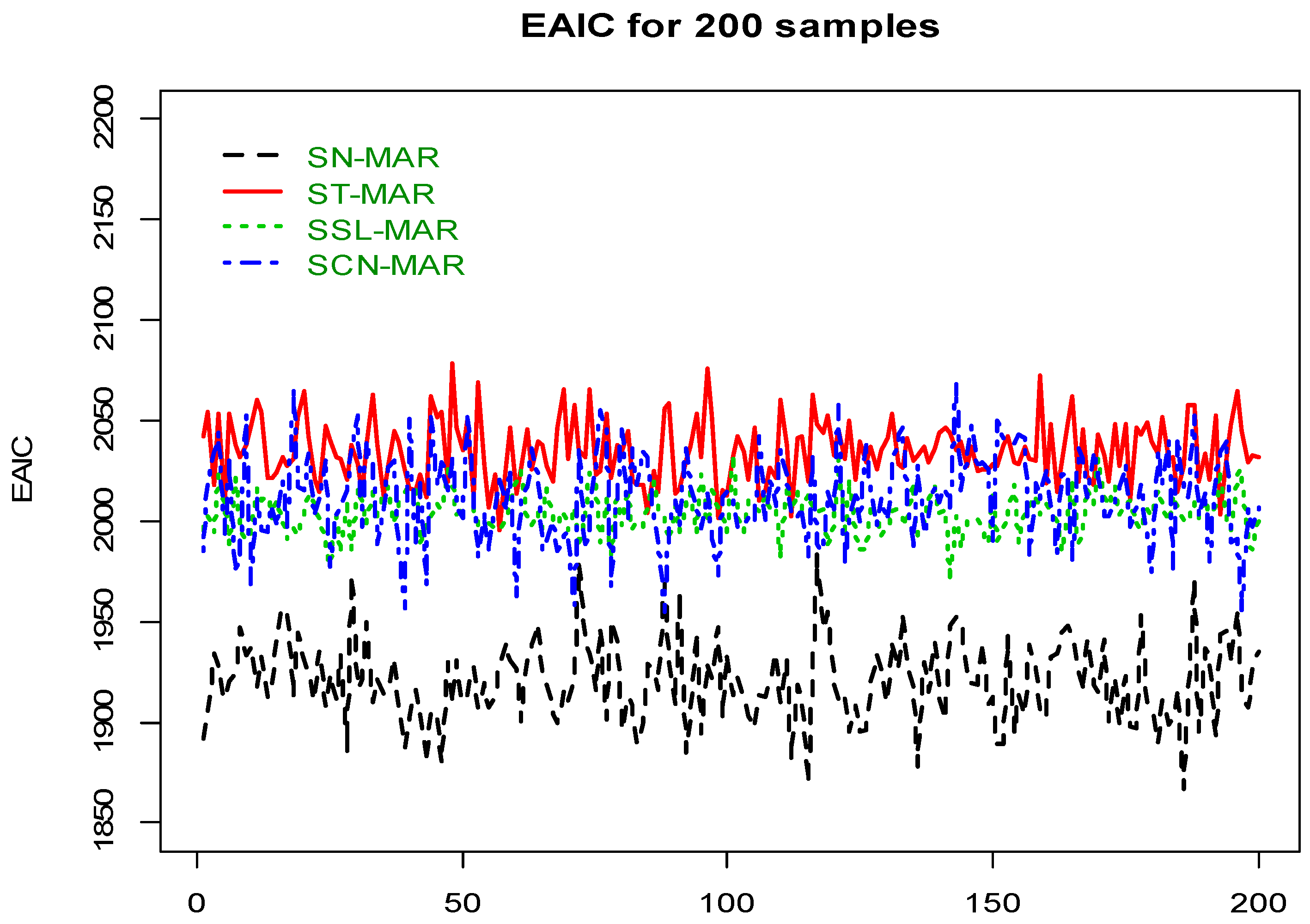
with the autoregressive coefficients in the first scheme, for which $\left\{{\epsilon }_{t1}\right\}$ be an i.i.d. sequence of $GH\left(\mu =0, \sigma =1,\gamma =-0.1, \overline{\alpha }=2,\lambda =1\right)$ with weak skewness, and $\left\{{\epsilon }_{t2}\right\}$ be an i.i.d. sequence of $GH\left(\mu =0, \sigma =1,\gamma =+3, \overline{\alpha }=2,\lambda =1\right)$ with strong skewness for innovations. The EAIC criteria of all Bayesian fitted SMSN–MAR models given in Figure 1, satisfies that the asymmetry and heavy-tailed members (i.e., ST–MAR, SSL–MAR and SCN–MAR models), especially ST–MAR, are the best fitted models in comparison with the light-tailed SN–MAR member.

4.3. Real Data

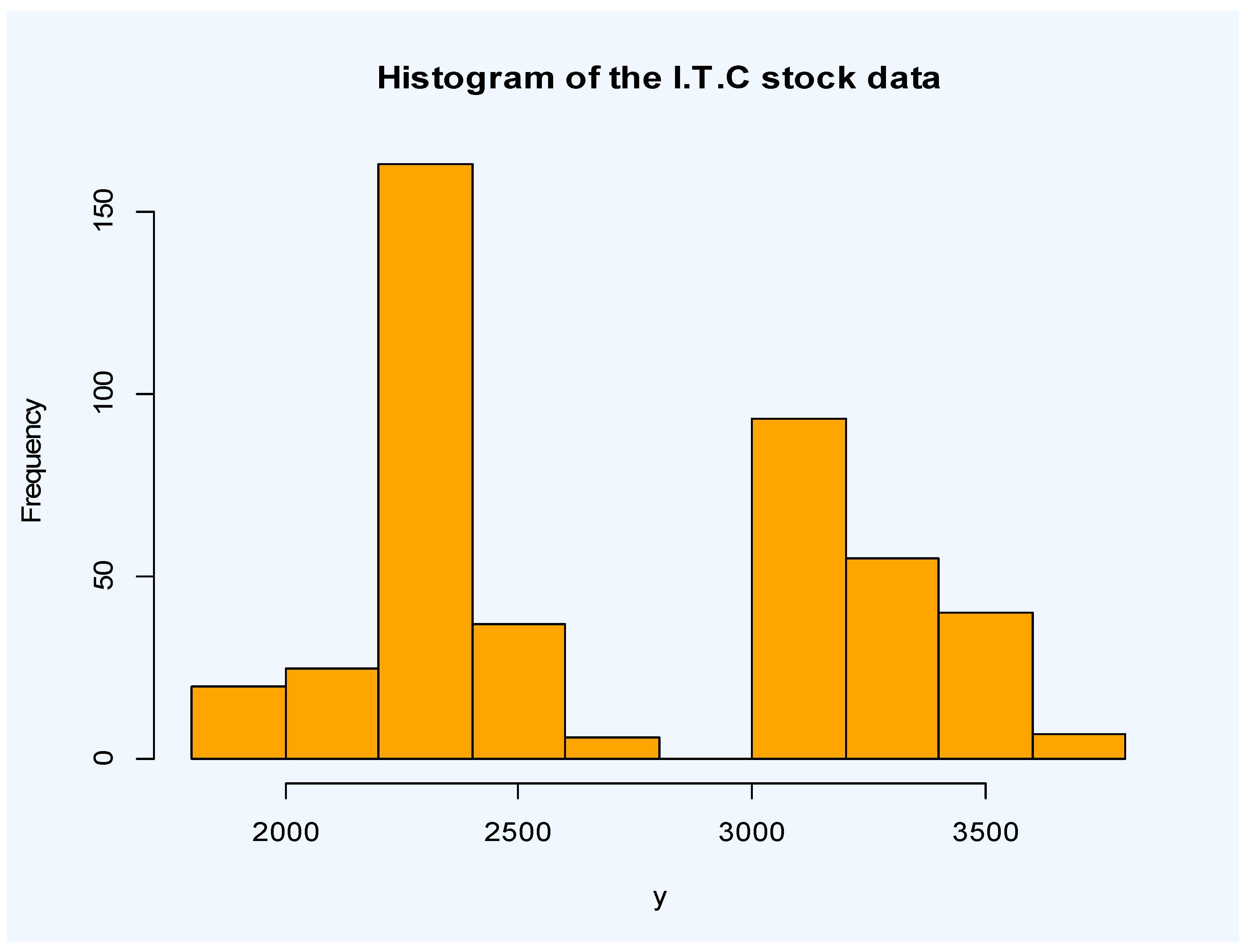
In this section, we consider the 446 daily observations of the closing price of Iran Telecommunication Company (I.T.C.) stock based on the Iranian Rial from 2011-07-02 up to 2013-07-02 (see data at Tehran securities exchange technology management company site: www.tsetmc.com). Original time series plot of the I.T.C. stock data $\left\{x_t\right\},$ where $x_t$ is the closing price at time$t,$ are given in Figure 2. It can be observed that the time series $\left\{x_t\right\}$ is not stationary. A histogram of the data is plotted in Figure 3.

Using the Box-Cox transformation with $\lambda =0$, and the difference with order of one, we have

$$y_t=x_t^{*}-x_{t-1}^{*}=\log \left(x_t/x_{t-1}\right),$$

(17)

where

$$x_t^{*}=\log x_t.$$

(18)

The time series $\left\{y_t\right\}$ has been plotted in in Figure 4. The Dickey–Fuller test verifies that the transformed time series data are stationary (p-value = 0.01).

The EAIC and EBIC criteria demonstrate that the best SMSN–MAR model has two components with order p₁ = 3 for the first AR component and p₂ = 1 for the second AR component. Using the proposed Bayesian approach, we fitted the N–MAR (GMAR), SN–MAR, ST–MAR, SSL–MAR and SCN–MAR models with g = 1,2,3 components. The Bayesian model selection criteria for them are given in

Table 2. Bayesian model selection criteria for the proposed SMSN–MAR(3,2) with various number of components $\mathrm{g}=1,2,3$.

Model	Number of Component (g)	EAIC	EBIC
N-MAR	1	3290.6352	3297.8210
	2	3067.3456	3291.9571
	3	3175.4758	3210.9882
SN-MAR	1	3262.7364	3271.7441
	2	3038.7464	3165.0641
	3	3175.7387	3183.7251
ST-MAR	1	2979.3748	2986.2951
	2	2816.8374	2887.3601
	3	2910.6364	2977.6781
SSL-MAR	1	3176.3647	3240.2990
	2	2997.0694	3099.8811
	3	3146.7564	3157.6441
SCN-MAR	1	3164.7564	3191.3452
	2	3009.3745	3097.3383
	3	3165.7564	3182.6013

Note: The best values (between all possible models) are indicated in bold.

. The Bayesian estimates (posterior mean) of the ST–MAR (3,2) (the best fitted) model parameters for the return series of the I.T.C. stock data are given in

Table 3. Bayesian estimates with standard deviations of the parameters of fitted ST–MAR (3,2) model for the return series of the I.T.C. stock data.

Component	Parameters	Bayesian Estimates	S.E.
First AR Component	${\pi }_1$	$0.5802$	$0.0156$
	${\phi }_{1,0}$	$0.0046$	$0.0100$
	${\phi }_{1,1}$	$0.1478$	$0.0304$
	${\phi }_{1,2}$	$-0.0487$	$0.0102$
	${\phi }_{1,3}$	$-0.0238$	$0.0011$
	${\sigma }_1^2$	$0.0036$	$0.0032$
	${\lambda }_1$	$1.0312$	$0.0193$
	$\mathit{\nu }$	$2.0034$	$0.0722$
Second AR Component	${\pi }_2$	$0.4198$	$0.0121$
	${\phi }_{2,0}$	$0.0030$	$0.0013$
	${\phi }_{2,1}$	$0.2256$	$0.0345$
	${\sigma }_2^2$	$1.0679$	$0.0094$
	${\lambda }_2$	$0.9017$	$0.0435$
	$\mathit{\nu }$	$2.0042$	$0.0847$

.

5. Conclusions

In this paper, we have considered the robust MAR models based on the scale mixtures of skew normal distributions, called SMSN–MAR, and a Bayesian approach to estimate the models’ parameters. These models are used for modeling non-linear time series data, which involve GMAR models, and offer greater flexibility than normal distribution. Numerical studies verified the good performance of the considered models and suitability of Bayesian estimates. A real data example demonstrated that SMSN–MAR models can be useful tools for non-linear and non-stationary time series modeling. In future studies, the researchers can consider cyclostationary or almost cyclostationary processes [26,27,28,29,30,31,32,33] with SMSN errors or mixture models based on these processes.

References

- Branco, M.D.; Dey, D.K. A general class of multivariate skew-elliptical distributions. J. Multivar. Anal. 2001, 79, 99–113. [Google Scholar] [CrossRef] [Green Version]
- Lindsay, B.G. Mixture models: Theory geometry and applications. In NSF-CBMS Regional Conference Series in Probability and Statistics; Institute of Mathematical Statistics: Hayward, CA, USA, 1995; Volume 51. [Google Scholar]
- Böhning, D. Computer-assisted analysis of mixtures and applications. In Meta-Analysis, Disease Mapping and Others; Chapman&Hall/CRC: Boca Raton, FL, USA, 2000. [Google Scholar]
- McLachlan, G.J.; Peel, D. Finite Mixture Models; Wiley: New York, NY, USA, 2000. [Google Scholar]
- Frühwirth-Schnatter, S. Finite Mixture and Markov Switching Models; Springer: New York, NY, USA, 2006. [Google Scholar]
- Mengersen, K.; Robert, C.P.; Titterington, D.M. Mixtures: Estimation and Applications; John Wiley and Sons: New York, NY, USA, 2011. [Google Scholar]
- Wong, C.S.; Li, W.K. On a mixture autoregressive model. J. R. Stat. Soc. Ser. B 2000, 62, 95–115. [Google Scholar] [CrossRef]
- Maleki, M.; Nematollahi, A.R. Autoregressive Models with Mixture of Scale Mixtures of Gaussian Innovations. Iran. J. Sci. Technol. Trans. Sci. 2017, 41, 1099–1107. [Google Scholar] [CrossRef]
- Ni, H.; Yin, H. A self-organizing mixture autoregressive network for time series modeling and prediction. Neurocomputing 2008, 72, 3529–3537. [Google Scholar] [CrossRef]
- McCulloch, R.E.; Tsay, R.S. Statistical inference of macroeconomic time series via markov switching models. J. Time Ser. Anal. 1994, 15, 523–539. [Google Scholar] [CrossRef]
- Glasbey, C.A. Non-linear autoregressive time series with multivariate Gaussian mixtures as marginal distributions. J. R. Stat. Soc. Ser. C 2001, 50, 143–154. [Google Scholar] [CrossRef]
- Wong, C.S.; Li, W.K. On a logistic mixture autoregressive model. Biometrika 2001, 88, 833–846. [Google Scholar] [CrossRef]
- Wong, C.S.; Chan, W.S. A student t-mixture autoregressive model with applications to heavy tailed financial data. Biometrika 2009, 96, 751–760. [Google Scholar] [CrossRef] [Green Version]
- Andrews, D.F.; Mallows, C.L. Scale mixtures of normal distributions. J. R. Stat. Soc. Ser. B 1974, 36, 99–102. [Google Scholar] [CrossRef]
- Maleki, M.; Wraith, D.; Arellano-Valle, R.B. Robust finite mixture modeling of multivariate unrestricted skew-normal generalized hyperbolic distributions. Stat. Comput. 2019, 29, 415–428. [Google Scholar] [CrossRef]
- Maleki, M.; Wraith, D. Mixtures of multivariate restricted skew-normal factor analyzer models in a Bayesian framework. Comput. Stat. 2019, 34, 1039–1053. [Google Scholar] [CrossRef]
- Zarrin, P.; Maleki, M.; Khodadadi, Z.; Arellano-Valle, R.B. Time series models based on the unrestricted skew-normal process. J. Stat. Comput. Sim. 2019, 89, 38–51. [Google Scholar] [CrossRef]
- Zeller, C.B.; Cabral CR, B.; Lachos, V.H. Robust mixture regression modeling based on scale mixtures of skew-normal distributions. Comput. Stat. Data Anal. 2010, 54, 2926–2941. [Google Scholar] [CrossRef]
- Maleki, M.; Wraith, D.; Arellano-Valle, R.B. A flexible class of parametric distributions for Bayesian linear mixed models. TEST 2019, 28, 543–564. [Google Scholar] [CrossRef]
- Wong, C.S.; Chan, W.S. Statistical Inference for Non-Linear Time Series Models. Ph.D. Thesis, University of Hong Kong, Hong Kong, China, 1998. [Google Scholar]
- Moravveji, B.; Khodadadi, Z.; Maleki, M. A Bayesian Analysis of Two-Piece Distributions Based on the Scale Mixtures of Normal Family. Iran. J. Sci. Technol. Trans. Sci. 2019, 43, 991–1001. [Google Scholar] [CrossRef]
- Brooks, S.P. Discussion on the paper by Spiegelhalter, Best, Carlin, and van der Linde. J. R. Stat. Soc. B 2002, 64, 616–618. [Google Scholar]
- Carlin, B.P.; Louis, T.A. Bayes and Empirical Bayes Methods for Data Analysis, 2nd ed.; Chapman & Hall/CRC: Boca Raton, FL, USA, 2001. [Google Scholar]
- Barndorff-Nielsen, O. Normal inverse Gaussian distributions and stochastic volatility modelling. Scand. J. Stat. 1997, 24, 1–13. [Google Scholar] [CrossRef]
- McNeil, A.J.; Frey, R.; Embrechts, P. Quantitative Risk Management: Concepts, Techniques and Tools; Princeton University Press: Princeton, NJ, USA, 2005. [Google Scholar]
- Mahmoudi, M.R.; Nematollahi, A.R.; Soltani, A.R. On the detection and estimation of the simple harmonizable processes. Iran. J. Sci. Technol. A (Sci.) 2015, 39, 239–242. [Google Scholar]
- Mahmoudi, M.R.; Maleki, M. A new method to detect periodically correlated structure. Comput. Stat. 2017, 32, 1569–1581. [Google Scholar] [CrossRef]
- Nematollahi, A.R.; Soltani, A.R.; Mahmoudi, M.R. Periodically correlated modeling by means of the periodograms asymptotic distributions. Stat. Pap. 2017, 58, 1267–1278. [Google Scholar] [CrossRef]
- Mahmoudi, M.R.; Heydari, M.H.; Avazzadeh, Z.; Pho, K.H. Goodness of fit test for almost cyclostationary processes. Digit. Signal Process. 2020, 96, 102597. [Google Scholar] [CrossRef]
- Mahmoudi, M.R.; Heydari, M.H.; Roohi, R. A new method to compare the spectral densities of two independent periodically correlated time series. Math. Comput. Simulat. 2019, 160, 103–110. [Google Scholar] [CrossRef]
- Mahmoudi, M.R.; Heydari, M.H.; Avazzadeh, Z. Testing the difference between spectral densities of two independent periodically correlated (cyclostationary) time series models. Commun. Stat. Theory Methods 2019, 48, 2320–2328. [Google Scholar] [CrossRef]
- Mahmoudi, M.R.; Maleki, M.; Pak, A. Testing the Difference between Two Independent Time Series Models. Iran. J. Sci. Technol. A (Sci.) 2017, 41, 665–669. [Google Scholar] [CrossRef]
- Mahmoudi, M.R.; Heydari, M.H.; Avazzadeh, Z. On the asymptotic distribution for the periodograms of almost periodically correlated (cyclostationary) processes. Digit. Signal Process. 2018, 81, 186–197. [Google Scholar] [CrossRef]
Figure 1.
EAIC criterion for 200 MAR samples based on the GH distributions.
Figure 2.
Time series plot of the I.T.C. stock from 2011-07-02 up to 2013-07-02.
Figure 3.
Histogram of the I.T.C. stock from 2011-07-02 up to 2013-07-02.
Figure 4.
Plot of returned I.C.T stock data.