
Abstract
BepiColombo has a larger and in many ways more capable suite of instruments relevant for determination of the topographic, physical, chemical and mineralogical properties of Mercury’s surface than the suite carried by NASA’s MESSENGER spacecraft. Moreover, BepiColombo’s data rate is substantially higher. This equips it to confirm, elaborate upon, and go beyond many of MESSENGER’s remarkable achievements. Furthermore, the geometry of BepiColombo’s orbital science campaign, beginning in 2026, will enable it to make uniformly resolved observations of both northern and southern hemispheres. This will offer more detailed and complete imaging and topographic mapping, element mapping with better sensitivity and improved spatial resolution, and totally new mineralogical mapping.
We discuss MESSENGER data in the context of preparing for BepiColombo, and describe the contributions that we expect BepiColombo to make towards increased knowledge and understanding of Mercury’s surface and its composition. Much current work, including analysis of analogue materials, is directed towards better preparing ourselves to understand what BepiColombo might reveal. Some of MESSENGER’s more remarkable observations were obtained under unique or extreme conditions. BepiColombo should be able to confirm the validity of these observations and reveal the extent to which they are representative of the planet as a whole. It will also make new observations to clarify geological processes governing and reflecting crustal origin and evolution.
We anticipate that the insights gained into Mercury’s geological history and its current space weathering environment will enable us to better understand the relationships of surface chemistry, morphologies and structures with the composition of crustal types, including the nature and mobility of volatile species. This will enable estimation of the composition of the mantle from which the crust was derived, and lead to tighter constraints on models for Mercury’s origin including the nature and original heliocentric distance of the material from which it formed.
1 Introduction
BepiColombo is the next mission to Mercury, made possible by collaboration between the European Space Agency (ESA) and the Japan Aerospace Exploration Agency (JAXA). The mission will build on the achievements of NASA’s Mariner-10 and MESSENGER missions, which revolutionized our understanding of Mercury but also raised many questions about this innermost planet of our Solar System, and to some extent about the formation of our Solar System itself as whole. Fuller understanding the current characteristics and origin of its inner end member will shed light on Solar System formation and evolution processes. As for many previous planetary missions, insights into planetary history can be gathered thanks to the thorough characterization of the physico-chemical properties of the planet’s surface (including its geology), its interior, and its close environment.
In 2008, members of the ESA’s BepiColombo Surface and Composition Working Group (SCWG) documented their intentions and aspirations for relevant science that could be conducted at Mercury by BepiColombo (Rothery et al. 2010). Although partially informed by preliminary results from MESSENGER’s first flyby, as well as Mariner-10’s three flybys in 1974-5, that work predated MESSENGER’s two subsequent flybys and, more importantly, MESSENGER’s March 2011 to April 2015 orbital campaign (Solomon et al. 2018, and references therein). Also, although BepiColombo’s instrument payload was already determined, the instruments themselves had not yet been assembled and some aspects of their capabilities were still evolving.
Here, in the light of the much improved knowledge of Mercury that is now available thanks to the completion of the MESSENGER mission, and knowing the capabilities of the instruments commissioned in space after BepiColombo’s launch on 20 October 2018, we discuss current knowledge and open questions about Mercury’s surface and composition. We discuss how BepiColombo’s comprehensive and complementary suite of instruments should be able to contribute to answering these questions, and describe some of the work that is underway to help us exploit BepiColombo data effectively.
2 Insights from the MESSENGER Era
MESSENGER imaging revealed the whole of the planet for the first time. Studies informed by MESSENGER data have considerably improved our knowledge of Mercury, its place in the Solar System (Solomon et al. 2018), and planet formation in general. They have also increased our awareness of what else we need to find out to further advance our understanding.
Previously, although Mercury’s high uncompressed density and intrinsic magnetic field demonstrated a large and partly molten iron core, the apparent low iron abundance (<3 wt% FeO) at the surface, suggested by lack of visible/near infrared Fe2+ crystal field absorption in silicates or glass phases, could be at least partly dismissed as a result of Fe-O bonds in silicate minerals having been broken by space weathering. This would turn some of the surface Fe into spectrally indeterminate nanophase iron particles (e.g., Hapke 2001; Warell and Blewett 2004; Penttilä et al. 2020). The latter could be responsible for the remnant crustal magnetization measured by MESSENGER at low altitudes (Johnson et al. 2015; Strauss et al. 2016). However, the total surface Fe abundance (independent of chemical state) was shown by MESSENGER X-ray and gamma-ray spectroscopy to be low. It ranges from 0.6 to 2.4 wt% across four northern hemisphere terrains, and the southern hemisphere average is 1.5 wt% (Nittler et al. 2011; Evans et al. 2012; Weider et al. 2014; McCoy et al. 2018). With confidence boosted by spacecraft gamma-ray spectroscopic studies of sampled asteroids, McCubbin et al. (2017) revisited MESSENGER gamma-ray spectroscopic data and concluded that this demonstrates a northern hemisphere O/Si ratio on Mercury of 1.2 ± 0.1, which is markedly lower than in other rocky bodies of the solar system. This implies that magmas originating from the mantle must have had a higher O/Si ratio than that observed at the surface, so and that any O/Si variability at the surface of Mercury might be linked to both the heterogeneity of mantle-derived melts and the degree of melt-crust interaction. It should however be noted that smelting described by McCubbin et al. (2017) is a secondary process resulting from the interaction between mantle-derived magmas and crustal graphite.
Understanding of the geochemical conditions during differentiation (i.e., while the core was segregating, and during possibly multiple episodes of crust formation) is necessary to reconcile the planet’s very high ratio of bulk metal (its core being presumably mostly Fe ± Ni, Si, S) with the iron-poor silicates and low oxygen abundance at its surface and in the mantle.
Before MESSENGER there was doubt as to how much of Mercury’s crust, even its smooth plains, is volcanic in origin (Wilhelms 1976; Strom 1997), but interpretation of MESSENGER images (e.g., Fig. 1) established beyond reasonable doubt that almost all the intact exposed crust is volcanic (e.g., Head et al. 2008; Byrne et al. 2018a, and references therein, and Denevi et al. 2018, and references therein). Modelling by Brown and Elkins-Tanton (2009) and Vander Kaaden and McCubbin (2015) showed that the low Fe content of Mercury’s primordial magma ocean would have resulted in too low a density contrast for any silicate phase to be sufficiently buoyant to form a flotation crust. The only feasible floating primary crust would have been a thin graphite layer (Vander Kaaden and McCubbin 2015), traces of which might now be evidenced by the ‘low reflectance material’ exhumed around some of the larger craters (Peplowksi et al. 2016; Klima et al. 2018). The thickness of the primary graphite crust, estimated at only a few 100 m by (Vander Kaaden and McCubbin 2015), is highly speculative and cannot be firmly estimated without additional constraints on carbon solubility in the core and in silicate melts under reduced conditions.

Part of Mercury’s Borealis Planitia seen in polar stereographic projection, and containing ample evidence of flooding by lava flows. Longitude marked at 20° intervals, latitude marked at 10° intervals. F is within a 140 km flooded basin at the southern edge of the plains. G marks two ghost craters whose rims are manifested only by wrinkle ridges. This is a standard MESSENGER enhanced colour view derived by principal component (PC) analysis of multi-spectral image data (red = PC2, green = PC1, blue = 433 nm/996 nm), on which the younger lava plains appear orange whereas the older terrain to the south (probably also emplaced as lava) appears bluer. (NASA/Johns Hopkins University Applied Physics Laboratory/Carnegie Institute of Washington)
The MESSENGER images showed tectonic shortening structures across the whole globe and brought the estimates of planetary radial contraction from photogeological mapping into line with the more extreme predictions from thermal models of 5-10 km (Byrne et al. 2018b). In addition, the highest-resolution imaging revealed some small young (<100 Ma?) structures and some small young (<100 Ma?) displacements on some large ancient structures, showing that global contraction probably continues into the present day (Banks et al. 2015; Watters et al. 2016). Although there are exceptions (Fig. 2) the dominant structural trend outside of impact basins is N-S, except polewards of 60° latitude (Byrne et al. 2018b). This finding is consistent with having been controlled by a blend of tidal despinning and thermal contraction (Klimczak et al. 2015), although it is not clear whether the effects of illumination bias (which emphasises N-S structures in mid-low latitudes) have been adequately accounted for (e.g., Fegan et al. 2017). Other than local fault-bend structures and small grabens on the crests of thrust-related anticlines, signs of extensional tectonics are limited to basin interiors where they convey information on basin isostasy and thermal contraction of lava flows (Byrne et al. 2018b).

MESSENGER Narrow Angle Camera (NAC) mosaic of an area within the Derain quadrangle (cylindrical projection). An atypical east-west stepped fault scarp (Calypso Rupes), cuts across smooth plains near 20° N. Note the locally-reduced crater density within some patches sharply-bounded by the downthrown (southern) side of the fault suggesting relatively recent ponding of small episodes of topographically constrained lava effusion, especially 40-41° E and 44° E. Note also the ubiquity of 20 km flooded craters except close to the southern (downthrown) side of the fault, where ponding would naturally be thickest allowing such craters to have become completely buried. (NASA/Johns Hopkins University Applied Physics Laboratory/Carnegie Institute of Washington)
One of MESSENGER’s most unexpected revelations was to provide multiple independent lines of evidence that Mercury’s surface, and by implication its crust and possibly mantle too, is rich in volatiles (Nittler et al. 2018, and references therein). Determining which volatiles are now (or were formerly) present, and in what abundances, is of fundamental importance for determining the distance from the Sun at which the material that now makes up Mercury condensed, as well as the history and nature of the collisions by which it grew. High volatile abundances could favour condensation significantly farther from the Sun than Mercury’s present orbit. A hit-and-run impact might be required to remove much of Mercury’s original silicate content (to explain its proportionately large core) without fully denuding of the surviving portion of volatiles although there are alternative explanations (Asphaug and Reufer 2014; Ebel and Stewart 2018; Cartier and Wood 2019).
Prime examples of evidence for volatiles include the following observations:
-
1)
the surface concentrations of Na, S, K, and Cl are similar to those on Mars (previously regarded as the most volatile-rich planet in the inner Solar System), and Na, S, and Cl abundances are at least an order of magnitude larger than on the volatile-depleted Moon (Nittler et al. 2018). Ebel and Stewart (2018) conclude that Mercury is anomalously enriched in S and that its bulk Cl and Na are probably enriched above chondritic values, whereas K is depleted but less so than for Earth.
-
2)
photogeologic identification of explosive volcanic vents in the form of non-circular holes of about 10 km size and 1 km depth (see later, Fig. 9). These are usually in the centre of a high albedo, spectrally red spot (a facula), several tens of km across with a diffuse outer edge, which is interpreted as an explosive eruption deposit (Byrne et al. 2018a and references therein). This is of relevance because explosive eruptions on the observed scale require the violent gaseous expansion of one or more abundant volatiles (Kerber et al. 2009).
-
3)
the discovery of ‘hollows’ (Fig. 3), which are (evidently young) steep-sided, flat bottomed depressions 10-20 m deep where 100 m to km wide patches of material have somehow been removed from the surface (Blewett et al. 2018 and references therein). The mechanism for hollow formation has not been determined (candidates include sublimation, thermal desorption, photon-stimulated desorption, and sputtering), nor do we know the identity of the species that is or are being lost. However, it is clear that whatever is being lost is not fully stable at present-day Mercury surface conditions and so it is, by definition, volatile-bearing.
Fig. 3 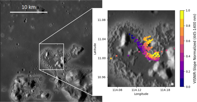
Hollows as seen in detail by MESSENGER in a 35 m/pixel NAC image. This example includes parts of the floor and central peak complex of Eminescu crater. The hollow-forming process appears to have eaten away at the surface around the peaks. In the enlargement on the right dots have been added to locate the mid-points of MASCS spectroscopic measurements, colour-coded to show the visible to near-IR slope (445 nm to 1400 nm) normalized by the slope of the Mercury reference spectrum calculated by Izenberg et al. (2014). Higher values of spectral slope are located on the hollow floors while lower values occur on their surrounding haloes. This hints at compositional differences, but the spatial resolution of these measurements is about 3 times larger than the dot size and the materials involved in hollows remain mysterious. We expect more informative data from BepiColombo. (From work in preparation by Barraud et al.)

Other observations consistent with the presence of volatile species include suggested down-slope mass movements (Malliband et al. 2019a), evidence for scarp-retreat at the edges of circum-Caloris ejecta blocks excavated from the lower crust or upper mantle below the basin (Wright et al. 2019a), and very low dip-angle thrusts (20° or less) which imply low friction coefficients on fault planes, possibly due to volatile overpressure during thrusting (Galluzzi et al. 2019). Known exospheric species include Na, Ca, Mg, Al, and K (McClintock et al. 2018), but the mechanisms by which these species are released from the surface into the exosphere are varied, depending on several factors. Their differing dawn-dusk and equator-pole asymmetries suggest a complex situation that might not be straightforwardly related to processes and composition observed or inferred at the surface (Milillo et al. 2020).
The significance of polar volatiles on Mercury is different from that of the widespread surface and crustal volatile species, which are almost certainly intrinsic to Mercury. Before MESSENGER, ground-based radar had mapped a radar-bright unit inside permanently-shadowed parts of polar craters, whose dielectric properties were consistent with any of water-ice or sulfur or supercooled silicates (Harmon and Slade 1992; Sprague et al. 1995; Harmon 2007). However, the MESSENGER neutron spectrometer data (Lawrence et al. 2013) showed a dip in both epithermal and fast neutron flux at high northern latitudes diagnostic of a hydrogen-rich substance (consistent with water, rather than sulfur and supercooled silicates). Reflectance measurements performed by the MESSENGER laser altimeter in north polar permanently-shadowed parts of craters, and eventually targeted imaging using light scattered into the shadows from the sunlit surroundings, showed surfaces with albedos distinctly different from that surrounding terrain. A few locations (notably, but not exclusively within the 112-km-diameter crater Prokofiev) had very high albedo consistent with water-ice, but numerous locations have very low albedo, interpreted to be complex carbon-bearing organic compounds (Chabot et al. 2018, and references therein). Both high- and low-albedo units are most simply interpreted as having been supplied as volatile molecules from comets or volatile-rich asteroids, or even from a single relatively recent impact event (Ernst et al. 2018). These molecules would have dispersed from impact sites until becoming confined in polar cold traps. If so, they are extrinsic to Mercury, and are likely to have no genetic relationship with the intrinsic crustal volatiles. It has been suggested that volatiles from volcanic outgassing could have contributed to polar volatile deposits but the fresh appearance and distinct surface reflectance of polar deposits would require outgassing to be sufficiently active at present or at least in Mercury’s recent past, which seems unlikely (Chabot et al. 2018).
3 Studies in Preparation for the BepiColombo Mission
3.1 Geological and Colour Mapping
Image coverage by Mariner 10 during its three flybys of Mercury allowed the production of 1:5M scale geological maps of the approximately 45% of the planet that had been adequately seen (see summary in Galluzzi et al. 2016). Geological maps of Mercury were not a planned deliverable of the MESSENGER project, although a global 1:15M scale geological map is in progress (Kinczyk et al. 2018).
The BepiColombo SCWG has set itself the goal of preparing geological maps covering the entire planet at 1:3M scale to establish an improved context for BepiColombo observations, and to help to prioritise targets for data acquisition and return. Data used are mostly from MESSENGER, supplemented by Mariner 10 images in cases where the different illumination conditions are helpful. So far, four of the fifteen quadrangles (H02, H03, H04, and H05) have been published (Galluzzi et al. 2016; Mancinelli et al. 2016; Guzzetta et al. 2017; Wright et al. 2019b), and several others are in progress (e.g., Galluzzi et al. 2018; Giacomini et al. 2017; Galluzzi 2019; Lewang et al. 2018; Malliband et al. 2019b; Pegg et al. 2019; Man et al. 2020; see Fig. 4). These morphostratigraphic maps (e.g., Fig. 5) adhere to protocols and standards recommended by the European Commission Horizon 2020 “Planmap” project (Rothery et al. 2018), which follow closely the established USGS protocols (Skinner et al. 2018) and symbology (FGDC 2006).

The status of Mercury geological mapping by SCWG in 2020. Green = ongoing, blue = scheduled. H01 is being mapped independently of SCWG by Ostrach et al. (2018)

Part of the 1:3 million scale map of the Hokusai quadrangle (H05), extracted from Wright et al. (2019b). The full quadrangle is 0°–90° E and 22.5°–65° N. This version distinguishes five crater degradation classes, whereas the version included in Fig. 4 distinguishes only three such classes, so colours used for crater materials are different
Planmap and allied efforts are also devoted to integrating morphological and spectral information by redefining geological units, through consideration of colour variation on spectral index maps as well as morphostratigraphic characteristics (e.g., Bott et al. 2019; Zambon et al. 2019). For example, the spectrally-defined ‘low reflectance material’ makes up some, but by no means all, of the morphostratigraphically-defined intercrater plains (Fig. 6; Whitten et al. 2014). There has also been some localized geomorphological mapping at up to about 1:300,000 scale in association with spectral studies of hollows (Lucchetti et al. 2018).

Enhanced MESSENGER colour image (as Fig. 1) of the Shakespeare quadrangle, H03 (Bott et al. 2019). This colour combination emphasises spectral units, such as the ‘low reflectance material’ (LRM) characterized by low reflectance and low spectral slope (dark blue in this rendering), and faculae (F), thought to be pyroclastic deposits, characterized by high reflectance and high spectral slope (orange in this rendering)
Upon completion of BepiColombo’s orbital mission, we anticipate that the unprecedented resolution of its imagery and compositional mapping will enable revision of quadrangle geological maps, and the production of larger scale maps of special interest areas.
3.2 Laboratory and Computational Studies to Support BepiColombo Surface Science
To understand the mineralogic diversity of a planet’s surface, it is essential to be able to interpret the remotely sensed spectral properties of the surface over a broad wavelength range.
The interpretation can be strong if analogue materials with systematic variation of both chemical properties (e.g., Fe/Mg in mafic solid solutions, variable SiO2 amount, different abundance of mixed minerals) and physical properties (e.g., grain size) have been investigated in laboratories with the same techniques. Moreover the environmental conditions (e.g. temperature) and weathering processes (e.g., solar wind, cosmic rays and solar photons) have to be taken into account. When spectral properties are determined under conditions similar to those of the anticipated observations, this enables models to interpret the spectral variation to be tested. Many activities associated with laboratory analysis and interpretation are ongoing within the SCWG.
Studies of emissivity and reflectance in the mid-infrared (MIR), and of reflectance in the visible to near-infrared (VNIR), have been done in air or low vacuum conditions, sometimes with variable acquisition geometry. These experiments are key to be able to attribute spectral features detected in the VNIR and MIR by BepiColombo to known mineral properties. We describe some examples below.
The emissivity of several analogues has been measured at the Planetary Spectroscopy Laboratory (PSL) of the Institute of Planetary Research in the German Aerospace Center (DLR) in Berlin, including rocks and silicates (Maturilli et al. 2008, 2014; Weber et al. 2016; Maturilli et al. 2017; Morlok et al. 2019), sulfides (Helbert et al. 2013b; Varatharajan et al. 2019), and graphites (Maturilli et al. 2019). Typically measurements in the spectral range of 7-14 μm are made at five temperatures (100, 200, 300, 400, 500 °C), in a low vacuum environment, intended to support mineral identification by BepiColombo’s thermal infrared instrument, MERTIS (see Sect. 4). The spectral reflectance of both fresh (before heating) and thermally processed (500 °C) analogues is measured from low to high phase angles (26-80°) across a wide spectral range covering 0.2-100 μm. During emissivity measurements, the analogues are continuously monitored using a webcam to study the chemical, physical, and morphological weathering of fresh analogues as they progress towards their thermally processed/weathered counterparts (Fig. 7).

Behaviour of MgS, a proposed volatile-rich mineral for hollows on Mercury (Vilas et al. 2016), is monitored while heating under thermal environment emulating Mercury at PSL during emissivity measurements where (a) shows the experiment setup before heating any sample (in this case MgS), b) MgS at 100 °C, c) MgS at 200 °C, d) MgS sputtered out while reaching the temperature of 250 °C, which is deposited in the side wall, thermopiles, and the rotating carousel
At Istituto di Astrofisica e Planetologia Spaziali (IAPS) laboratories in Rome, studies on possible low-iron analogues are ongoing to test the capability to document the composition of iron-bearing minerals at low abundances (e.g., Serventi et al. 2018), and properties of glasses with variable composition (Carli et al. 2018). Such tests have been performed with special attention in the VNIR where SIMBIO-SYS (see Sect. 4) will work. Various models (including Gaussian deconvolution of spectra and modelling by radiative transfer and intimate mixing) have been applied to retrieve mineralogical composition of mineral mixtures with igneous-like rock forming minerals and glasses (e.g., Carli et al. 2018; Serventi et al. 2018). For some of these materials the reflectance properties have been measured during various temperature ramps with a confocal microscope set-up in a nitrogen flowed environment in collaboration with Institut d’Astrophysique Spatiale (IAS), Orsay, and Laboratoire d’études spatiales et d’instrumentation en astrophysique (LESIA), Paris (e.g., Bott et al. 2018).
For modeling the spectral properties of minerals in VNIR and MIR wavelengths, the University of Helsinki has developed computational light-scattering methods to be used in the inversion of optical constants and in simulating spectral reflectance (Martikainen et al. 2019; see also Muinonen et al. 2018; Väisänen et al. 2019). The methods can take into account the size distribution of regolith particles and the effects of different ratios of surface-based and volume-based scattering. Furthermore, nanophase iron or carbon particles can be included as small diffuse scatterers in a thin surface layer of the regolith particles (Penttilä et al. 2020). Darkening of the mineral spectra is particularly relevant due to the harsh space-weathering conditions on Mercury.
Elsewhere, there are studies on space weathering effects caused by macro to micro impactors. For example, at the Westfälische Wilhelms Universität Münster, Germany, analogue material can be altered with a pulsed 193 nm ArF UV excimer laser or by an IR laser (Weber et al. 2019). The run products are analyzed in NIR and MIR. In collaboration with the Museum für Naturkunde in Berlin, MIR spectra of glasses produced with an 8 kW infrared fibre laser and pulsed laser irradiation experiments with a 300 W Nd_YAG laser are obtained (Morlok et al. 2020).
In addition to the laser-altered analogue material, classic shock recovery experiments (experimental set-up described in Stöffler and Langenhorst 1994) are conducted in collaboration with the University of Bern to simulate impacts into porous regolith material. Monomineralic porous powder samples are shock-altered, and run products are investigated in the MIR range (Stojic et al. 2019).
Thanks to the facilities and expertise at IAS and the SOLEIL IR line, investigations of the effects of space weathering on several materials, glasses and minerals, are ongoing (e.g., Carli et al. 2018). It is planned to use the SIDONIE mass separator at Centre des Sciences Nucléaires et de Sciences de la Matière (CSNSM) Orsay to measure minerals, meteorites and synthetic Mercury-like analogues, to simulate the effects of the solar wind, with implanting of various ions (e.g., Ar, He, …).
Other space weathering simulations are expected to be performed by the Planetology Laboratory University of Salento (PLUS), recently University Section of INAF, irradiatiating powders of analogues with a KrF excimer laser, working at a wavelength of 248 nm. The irradiated materials will be analyzed using directional-hemispherical reflectance spectra collected from the UV up to MIR (with two set-ups: 0.25–2.5 μm and 2.0–25. 0 μm).
In the X-ray region of the spectrum, “regolith effects” (mainly the grain size and porosity of the surface) can lead to changes in the observed intensity of different energy X-rays as a function of the phase angle of the observation (Maruyama et al. 2008; Näränen et al. 2009; Weider et al. 2011). Such phase-angle effects were observed empirically in Fe/Si and Cr/Si measurements made by the MESSENGER X-ray Spectrometer (Weider et al. 2014; Nittler et al. 2020). To fully understand the influence of these effects on data returned by the MIXS instrument (Sect. 4), experiments will be undertaken at the University of Leicester using flight-like versions of the electronics and detector systems on board MIXS to study Mercury analogue materials (Bunce et al. 2020). Spectral modelling at the University of Helsinki will be used to constrain the influence of grain size, porosity and viewing geometry on the data returned from these experiments, seeking to maximise the scientific return from in-flight data. The modelling was initiated in Parviainen et al. (2011), in which olivine basalt was studied using first-order fluorescence in discrete random media of particles. For example, in Fig. 8 the methods are applied to a regolith composed of large plagioclase particles, illustrating regolith effects on X-ray intensity.

Simulated fluorescence line ratios of Ca K\(\alpha \)/Al K\(\alpha \) from a porous, infinitely thick slab composed of close-packed spherical plagioclase particles of equal size (radius \(r\)). FPE refers to the Fundamental Parameter Equation of X-ray fluorescence (Van Grieken and Markowicz 1993; Clark and Trombka 1997), which is an analytical approximation for a first-order X-ray fluorescence from a smooth, infinitely thick, solid slab of plagioclase. The results are normalized to unity at the emergence angle of 0° as counted from the outward normal direction of the surface element
In the gamma-ray energy range, the MGNS team performed experimental testing of methodology of the gamma-ray space science measurements with samples prepared as analogs of Mercurian surface material. The experimental research was performed at the Laboratory of Neutron Physics at the Joint Institute for Nuclear Research (JINR, Dubna) by physicists from Space Research Institute (IKI, Moscow, Russian Academy of Sciences). The samples include chemical elements that are the main rock-forming elements in the Mercurian surface layers: Si, Al, Ca, Fe, Ti, Mn, Cr, Cl etc. The results of these experimental measurements have been used to compile a database of the reference gamma-ray lines of basic rock-forming elements that can be identified by means of a MGNS gamma-ray spectrometer based on a CeBr3 scintillation crystal. This will be used to analyze and interpret gamma-ray data from the MGNS space-science experiments in ordbit about Mercury (Kozyrev et al. 2018). Also, a comprehensive programme of numerical simulations of the energy spectra of gamma-rays will be performed for different types of the surface composition. The results of these calculations will be used for identification of detected nuclear lines and for estimation of abundance of corresponding elements in the shallow subsurface (Masarik and Reedy 1996; Mitrofanov et al. 2020).
4 BepiColombo Spacecraft and Instruments
BepiColombo consists of two scientific spacecraft that, after arrival at Mercury, will be placed in separate polar orbits (Benkhoff et al. 2020; Murakami et al. 2020). The European Space Agency, ESA, will retain control of the Mercury Planetary Orbiter, MPO. This spacecraft is especially relevant to Mercury’s surface and its composition, and will have an initial low-latitude periherm of about 480 km above the surface and an apoherm of about 1500 km above the surface. The initial periherm will be north of the equator, but is expected to drift southwards as the mission progresses. This will permit equally good coverage of northern and southern hemispheres, in contrast to MESSENGER that had a much more eccentric orbit with a periherm latitude largely confined to between 60° and 84° N (Solomon and Anderson 2018). The MPO payload, including names and acronyms, is summarized in Table 1.
The other orbiter, Mio (formerly known as the Mercury Magnetospheric Orbiter, MMO), will be controlled by the Japan Aerospace Exploration Agency, JAXA, after it has been delivered into orbit about Mercury. This spacecraft will have an initial periherm at about 600 km and an apoherm of about 12,000 km. It is equipped to study magnetic and electric fields and the particle environment (Murakami et al. 2020). After 2-3 years in orbit Mio’s periherm could have drifted sufficiently low for it to be able to detect crustal magnetic anomalies.
Following Mercury orbit insertion in December 2025, full MPO science operations are expected to be underway by May 2026, whereas Mio will already be in its science orbit and should be fully functional at an earlier date. The nominal science mission is one year, but if the spacecraft remain healthy they could continue for a few years longer. MPO’s periherm is expected to become lower at decreasing rate (reaching about 280 km by 1 January 2028), whereas Mio’s will become lower at an increasing rate (reaching about 330 km by the same date). The capabilities of individual instruments are addressed in relevant papers in this volume. Among the entire BepiColombo payload, the experiments of most relevance to determining surface properties (composition, physical state, topography) are BELA, MERTIS, MGNS, MIXS, and SIMBIO-SYS, whereas PHEBUS and SERENA might be able to quantify the volatile species being released from the surface.
5 Science Questions
We describe below the main science questions concerning Mercury’s surface and composition that we hope BepiColombo will be able to answer. We comment on the relevance or context of each question, and point out the expected contributions from each instrument. Few if any questions can be well addressed by a single instrument, and synergies between instruments will be of great importance. More details on the capabilities of each experiment are given in the relevant experiment-specific papers in this volume.
The questions listed here draw on, but do not directly map onto, the BepiColombo project’s Science Traceability Matrix for each instrument. The general ordering of the questions here proceeds from the specific toward the more general.
5.1 What Is the Elemental Composition of the Surface and Crust?
MIXS and MGNS are the two MPO instruments that will make direct measurements of surface elemental abundances, by imaging X-ray spectroscopy and non-imaging gamma-ray spectroscopy of the very shallow subsurface, respectively (Bunce et al. 2020; Mitrofanov et al. 2010). In addition, the MGNS neutron spectrometer will provide measurements of neutron flux at different energies, from which abundances of hydrogen can be inferred. A low-altitude opportunity to detect neutron moderation attributable to carbon was achieved by MESSENGER’s neutron spectrometer (e.g., Peplowksi et al. 2016), which the MGNS neutron spectrometer may not be able to repeat. However if the opportunity arises we would hope to confirm the interpretation by a detecting consistently increased emission of carbon nuclear lines using the MGNS gamma-ray spectrometer.
The MPO’s near-equatorial periherm will potentially result in finer spatial resolution data than MESSENGER at all latitudes. Moreover, both poles will be well mapped. This is in contrast to the equivalent experiments on MESSENGER that returned no spatially resolved element abundance data over mid- to high-southern latitudes, due to its periherm being always at a high northern latitude and its apoherm (at the opposite southern latitude) being about ten times more distant than MPO’s will be, with the result that the range to the surface was much larger in the south.
The gamma-ray spectrometer component of MGNS will detect radioactively-emitted gamma rays from U, Th and K, and gamma rays emitted as a result of cosmic ray bombardment of minerals containing Na, Fe, Ti, Al, Mg, Si, Ca, C and O. Achievable spatial resolution by MGNS over the lifetime of the mission will be about 400 km per pixel for most elements, but may be as coarse as global for weak emitters such as Na, Ti, and Ca. MIXS will provide much better spatial resolution (at best a few km per pixel for MIXS-T, a few tens to hundreds of km per pixel for MIXS-C), but comparisons of abundance measurements between the two experiments will be of interest because of the larger sampling depth (top tens of cm) achieved by gamma-ray spectroscopy compared with the tens of μm sampling depth of X-ray spectroscopy.
The X-ray spectrometer, MIXS, will detect more elements in total than MGNS. Moreover, one of its two components (MIXS-T) is an X-ray telescope capable of sub-10 km spatial resolution near periherm during flares, when the incident solar X-ray flux will be of sufficiently high intensity. The achievable pixel size will usually be coarser than this, varying for each element, the flare state of the Sun, and range to the planet’s surface. Potentially mappable elements are Si, Al, Fe, Mg, Ca, S, Ti, Cr, Mn, Na, K, P, Cl, Ni, and O, of which the first eight were spatially resolvable (across parts of the globe only) by MESSENGER’s X-Ray Spectrometer (XRS), which also placed an upper limit on Mn (Nittler et al. 2018). The 277 eV K\(\alpha \) fluorescence by C is technically below the lower energy threshold of the MIXS focal plane assembly after the predicted in-space radiation exposure, but actual detector performance, which will be assessed in orbit, may allow C to be detected (Bunce et al. 2020). The ability of MIXS to map both Si and O will allow it to evaluate spatial variations of the O/Si ratio of crustal rocks and estimate the abundance of Si-rich, Si-Fe alloys at the surface, which McCubbin et al. (2017) suggested to be 12-20%. This will cast light on whether these phases are primary or secondary, for example formed by smelting when magma encountered graphite in low-reflectance material and perhaps space weathering as proposed by McCubbin et al. (2017). Mineralogical mapping by MERTIS will also be useful to constrain these processes.
On the basis of MESSENGER XRS and Neutron Spectrometer (NS) data it is possible to distinguish a few apparently distinct ‘geochemical terranes’ (Nittler et al. 2020), including a ‘high-magnesium region’ that except for some potential tectonic boundaries (Galluzzi et al. 2019) has no obvious visual identity in the landscape (e.g., Weider et al. 2015; Peplowksi et al. 2015; Frank et al. 2017). BepiColombo will use more elements to map geochemical terranes. It will do this with spatial resolution better suited to localizing their edges, and thus help to clarify whether their boundaries are confined by impact basins, or controlled by tectonic features or flow-fronts.
Significant geochemical variability is however observed even within individual provinces, which indicates that they formed through long-lasting igneous events (Weider et al. 2015). Better understanding of the origin of erupted products as well as their short- to long-wavelength geochemical heterogeneity requires accurate measurements at high spatial resolution. Currently available XRS data from MESSENGER have data gaps for some elements (Ca, S, Fe) in the northern hemisphere and the resolution in the southern hemisphere is poor for all elements (Weider et al. 2015; Nittler et al. 2018, 2020). The additional elements, higher spatial resolution, and more uniform coverage planned for MIXS lead us to expect further insights and surprises from BepiColombo.
5.2 What Is the Mineralogy of the Crust?
Knowledge of the mineralogy of a planet’s crust is useful for understanding not just how the minerals formed (the influences of fractional crystallization and crustal assimilation), but also deep magmatic processes such as the mechanisms and degree of mantle melting. Mineralogy also has a crucial bearing on the physical properties of the crust, and hence is relevant for understanding geophysical data. The mineralogy of Mercury’s surface is currently inadequately known, because of the difficulties and ambiguities in interpreting the spectral data. Ground-based and airborne mid-infrared telescopic studies indicate a regolith composition dominated by plagioclase, pyroxene and olivine with minor feldspathoids, garnet, amphibole, rutile and perovskite. Spectra also show similarity to intermediate to (ultra)mafic rocks. Grain size is mostly finer than 25 μm. However, these studies integrate the signals of large regions (\(10^{4}\) – \(10^{6}~\text{km}^{2}\)) and have low signal to noise ratios due to atmospheric interference (Donaldson-Hanna et al. 2007; Sprague et al. 1994, 2000, 2002, 2007, 2009; Sprague and Roush 1998; Emery et al. 1998; Cooper et al. 2001).
MESSENGER spectroscopic data provide a few further hints about Mercury’s surface mineralogy. One of the first attempts to derive a global mineralogy of Mercury’s surface was presented by Wurz et al. (2010) based on all data available at the time, including Mariner 10, the early (flyby) MESSENGER results, and ground based observations. This early model presents Mercury surface mineralogy as a mixture of feldspar, pyroxene, olivine, metallic iron and nickel, and a few wt% of sulfides, ilmenite, and apatite.
The main mineralogic insights provided by MESSENGER come from indirect approaches such as calculating normative mineralogies based on the measured elemental abundances (Stockstill-Cahill et al. 2012; Vander Kaaden et al. 2017) and high temperature experiments (Charlier et al. 2013; Namur and Charlier 2017). These methods allow the identification of likely minerals, but modal abundance and the crystallinity of the rocks (glass vs. crystals) are largely unknown. Experiments give a direct insight into mineralogy and petrography, but are time consuming and impractical to perform across a large variety of bulk compositions. Normative calculations are much faster, but represent only a first approximation to the actual mineralogy because of two necessary assumptions: 1) that what is seen in each pixel represents a single rock type (i.e. that the regolith in the pixel is derived from a uniform source, which is in most cases not true); and 2) that crystallization has proceeded under conditions of equilibrium (i.e., no fractional crystallization or crustal assimilation). The peculiar compositions measured on Mercury make this approach even less dependable.
Other peculiar aspects of Mercury’s crustal mineralogy concern the existence of sulfide minerals, inferred from the high sulfur abundance, coupled with the low abundance of O. What sulfide species are involved is currently unknown. The low Fe content of Mercury’s crust is not consistent with FeS being the main sulfur host (Cartier and Wood 2019). In contrast, the correlation between Ca/Si and S/Si ratios discovered by MESSENGER suggests the presence of CaS (Weider et al. 2011), although experiments have shown that S forms complexes preferentially with Mg in silicate melts under Mercury conditions (Namur et al. 2016a). Associated with the high S abundance, the low O/Si ratio derived from MESSENGER gamma-ray spectroscopy (McCubbin et al. 2017) suggests that 12-20% of the surface materials on Mercury are Si-rich, Si-Fe alloys.
MPO is equipped with instruments that are better suited for mineral identification than MESSENGER was. VIHI, the visible and near IR imaging spectrometer component of SIMBIO-SYS has a spectral range extending to 2000 nm (Cremonese et al. 2020) whereas MESSENGER’s non-imaging spectrometer (Mercury Atmospheric and Surface Composition Spectrometer, MASCS) cuts off at 1450 nm. VIHI’s enhanced near-infrared range will bring additional electronic transitions of ferrous iron and other transition elements into scope (e.g., Burns and Burns 1993), potentially enabling solid solution of olivines and pyroxenes to be characterized. However, MESSENGER MASCS data showed little variation in the 300 – 1450 nm range (Izenberg et al. 2014) possibly because of the low total Fe content of Mercury’s surface.
VIHI will permit global coverage of Mercury’s surface with an average pixel scale of better than 500 m, and the ability to image selected targets at a pixel scale of better than 120 m (Flamini et al. 2010; Capaccioni et al. 2010, Cremonese et al. 2020). The pixel scale will depend on the MPO orbit that will change during the mission, but the consistently much higher spatial resolution is expected to be a key factor in the identification of any spatially variable mineralogies present on Mercury’s surface.
Perhaps more significantly, MPO has a 7-14 μm thermal infrared imaging spectrometer as the main component of MERTIS (Hiesinger et al. 2020), allowing identification and characterization of mineral phases by means of the cation-anion and lattice vibrations of crystalline structure (Farmer 1974). This will provide thermal infrared evidence of fundamental vibrations in silicates, independently from VNIR absorptions caused by the presence of transition elements. Pyroxenes and olivines should be distinguishable regardless of Fe content, and even the complex spectral features of the feldspar group (Reitze et al. 2020) or other phases lacking transition elements are capable of being determined. It is likely that metallic Si and Si-Fe alloy could be detectable through emissivity features (whose width is likely to be temperature dependent) in the MERTIS spectral range (e.g., Abedrabbo et al. 1998).
The harsh thermal environment and high diurnal thermal range on Mercury can lead to shifts in the position of characteristic features for silicate minerals at the TIR wavelength ranges (Helbert et al. 2013b; Ferrari et al. 2014) due to changes in the lattice volume space. Furthermore, heating-related features such as structural order/disorder effects in the abundant feldspar can be detected in the MIR (Reitze et al. 2020). The combination of simultaneous temperature measurement by the MERTIS radiometer plus spectral measurements will allow this effect to be studied in detail. The available laboratory data (Maturilli et al. 2014; Ferrari et al. 2014) show that the thermal effects are variable in different crystals but well understood for the main minerals that are thought to characterize the hermean surface.
In contrast the NIR and visual spectral range is strongly affected by a loss of spectral contrast as observed for example for sulfides (Helbert et al. 2013a; Varatharajan et al. 2019), labradorite (Helbert and Maturilli 2009), and komatiite (Maturilli et al. 2014), although wavelength shifts in spectral absorptions are likely. Hence coupling the SIMBIO-SYS VIHI and MERTIS datasets will be pivotal for correct interpretation of Mercury’s mineralogical surface composition. Together with the deblurring thanks to improved spatial resolution of elemental mapping that MPO will provide, we expect to develop a much better grasp of Mercury’s mineralogy than before.
5.3 What Are the History and Mechanisms of Effusive Eruption?
MESSENGER established with little doubt that the vast majority of Mercury’s surface is constructed from large volume, low viscosity lava flows. Even parts of the intercrater plains, which is the collective term for the oldest widespread unit, retain traces of ghost craters demonstrating burial of craters by lava followed by subsidence or regional horizontal compressive stress to allow topographic re-expression of the buried crater rim. Smooth plains, which extend over nearly 30% of the globe (Denevi et al. 2013), contain numerous ghost craters and wrinkle ridges (Fig. 1). Although large scale effusive volcanism waned about 3.5 billion years ago (Byrne et al. 2016), smooth crater floor material, which is often clearly younger than its host crater, is very likely lava rather than impact melt (Prockter et al. 2010; Marchi et al. 2011; Fegan et al. 2017). Additionally, small smooth patches, notably some that are ponded against fault scarps (Malliband et al. 2018; Fig. 2), provide plausible evidence that the waning of effusive volcanism after the first fifth of the planet’s history was subsequently drawn out at smaller scales over billions of years. BepiColombo will either increase our confidence in this interpretation, or force us to revise our opinions.
The source vents for plains-forming lavas on Mercury (including within basins <200 km diameter) have not been convincingly located, and it is reasonably assumed that the lavas have buried their own source vents (Byrne et al. 2018a). Four ‘coalesced depressions’ illustrated by Byrne et al. (2014) are not necessarily effusive vents (one alternative is that they are sites of explosive eruptions, lacking visible faculae). Some broad channels with streamlined ‘islands’ are known near the southeast margin of the smooth plains of Borealis Planitia (Byrne et al. 2014), and high-resolution, high sun-angle images reveal some intriguing surface morphologies at sites where flows have descended topographic steps in and around the Caloris basin (Rothery et al. 2017). Rothery et al. (2017) argued on the basis of the patchiness revealed in MESSENGER enhanced colour images of the circum-Caloris plains that flow lengths are more likely to be hundreds rather than thousands of km. We expect that improved coverage by suitable SIMBIO-SYS images will reveal more detail and further examples, enabling ambiguous lava features to be interpreted with better confidence. In combination, STC and HRIC may also reveal flow boundaries and lava tube skylights that have so far proved elusive (Byrne et al. 2018a); whereas VIHI and MERTIS might distinguish lava flows of different mineralogical composition.
We also look ahead to better and more comprehensively imaged ghost craters, whose study will enable estimates of flow thickness (and hence volume), and for use in quantifying the age difference between pre- and post-lava surfaces. More robust identification of ‘small, young’ lava patches will enable better constraints on whether or not the waning phase of effusive eruptions persisted (like explosive eruptions, see next section) into Kuiperian times.
There is a current disagreement over whether there exists on Mercury a mappable unit (‘intermediate plains’) whose morphology is intermediate between intercrater plains and smooth plains, and, if so, whether or not this shows spectral variability different from either of the other two units (Galluzzi et al. 2017). Where such a unit is mapped, it is unclear whether it represents simply lava plains of intermediate age or else thin flow units that have incompletely obscured pre-existing craters on the intercrater plains (e.g., Whitten et al. 2014; Galluzzi et al. 2017; Wright et al. 2019b). This issue is unlikely to be settled until we have higher resolution image coverage from BepiColombo.
5.4 What Are the History and Mechanisms of Explosive Eruption?
The majority of Mercury’s explosive volcanic vents are on the floors, rims, central peaks or peak rings of impact structures, on a fault, or within 20 km of a fault (Klimczak et al. 2018). These explosive eruptions could not have happened unless there were sufficient volatiles to expand explosively as a gas (Kerber et al. 2009). Better documentation of the nature and history of these eruptions should improve our understanding of the quantities and sources of volatiles involved in eruptions, the most likely plumbing systems and whether volatiles must be recharged between successive eruptions (Pegg et al. 2020). Rothery et al. (2014) studied one of the best-imaged vents, in the middle of what has now been named Agwo Facula in the southwest of the Caloris basin. These authors showed that the 30 km long pit contains about 9 individual vents lying within a common rim and in some cases separated by narrow septa (Fig. 9). They likened this to a ‘compound volcano’ on Earth where the locus of eruption has migrated over time, and pointed out that textural contrasts between the vents imply a series of eruptions conceivably spread over a considerable (billion year) time scale. If this interpretation is correct, the surrounding facula is the product of a series of eruptions rather than of a single event. Thomas et al. (2014b) showed that, where documented by MESSENGER laser altimetry or stereo imaging, vents are 1-3 km deep and the surrounding facula is rarely thick enough to constitute a perceptible topographic cone.

Agwo Facula and the compound volcanic vent at is centre. Main image: enhanced MESSENGER colour image (as in Fig. 1), centred on the Agwo Facula vent. The facula is the diffuse edged orange region surrounding the vent (another facula, Abeeso, overlaps it on the southwest). Insert: High resolution MESSENGER NAC image of the vent, revealing its compound nature. Different impact crater densities and topographic sharpness are revealed in the various component vents within in
Jozwiak et al. (2018) also recognised the likelihood of multiple phases of eruption from non-equidimensional vents. In addition, Pegg et al. (2020) suggested that as many as 70% of 288 identified vents are probably compound vents. Few compound vents were imaged by MESSENGER as clearly as the Agwo Facula example, so much remains to be discovered by BepiColombo.
The long-term recurrence of explosive eruptions at any vent site has implications for the supply of volatiles, and the intervals between eruptions are relevant to the rate at which volatiles are locally recharged. Considerations of recharge apply to the site of magmagenesis if the volatiles arrive with the magma, or to some layer in the crust (or even just the regolith) if the ascending magma gains its volatiles from those units during approach to the surface. Analysis of faculae using MESSENGER’s non-imaging spectrometer (MASCS) demonstated the value of spectral parameters in defining the limits of these diffuse-edged features and confirms that they are larger than was apparent when first identified on MESSENGER fly-by images (Besse et al. 2020). High-resolution MASCS data are limited to discrete profiles (usually oriented close to north-south), so VIHI imaging spectroscopy is likely to be valuable in better constraining facula dimensions.
In addition to the compositional data described in Sect. 5.6, an important contribution by BepiColombo to understanding the nature of the explosive processes, and the longevity and recurrence of their activity, will be to image more of them in higher resolution so that cross-cutting (and hence age) relationships can be established. This will also allow age-related muting (mantling?) of surface textures to be better discerned and documented. Additionally, stereo imaging by SIMBIO-SYS STC and laser altimetry by BELA will give improved measurements of vents’ steep internal slopes.
Explosive vents generally cut through, and their faculae generally overlie, plains or crater floor material. The youngest vents cut through terraces inside Kuiperian age craters (Thomas et al. 2014c; Jozwiak et al. 2018), and so must have been active within the past billion years, or even within the past 280 million years on the chronology of Banks et al. (2017). Vent interiors are far too small to permit reliable model surface ages from cratering statistics, but comparisons within a compound vent in the superposed density of <100 m diameter craters never contradict the time sequence deduced by cross-cutting relationships, and can at least indicate over what fraction of a vent’s age the activity is likely to have taken place. There are no candidate explosive vents that demonstrably pre-date smooth plains, but if more detailed study reveals evidence of early Calorian or Tolstojan ages for some vents, such a discovery would at least partly overturn the current impression that volcanism switched from effusive to explosive during the Calorian (Goudge et al. 2014; Thomas et al. 2014c). On the other hand better-defining the upper age of pyroclastic material with HRIC data could constrain the potential contribution of intrinsic volatiles to polar deposits in permanently shadowed regions. The thermal inertia maps provided by MERTIS will provide insights into the grain size variation around volcanic vents which would provide constraints on models for explosive volcanism on Mercury.
Additionally, stereo imaging by SIMBIO-SYS STC and laser altimetry by BELA will give improved measurements of the steep internal slopes of vents. By sampling of the return pulse BELA has the capability for determining the pulse broadening that is indicative of slope and roughness at the footprint diameter of about 20 to 50 m (changing with MPO altitude). By correcting for slopes from a sequence of laser spots, the pulse-spreading is a measure for surface roughness on the footprint scale. Correlation (or anti-correlation) with geologic units will be indicative of processes that have shaped the surface on these small scales.
The locations of candidate volcanic vents are already well known, simplifying the task of locating BepiColombo data likely to be of relevance. Thomas et al. (2014b) catalogued vents at 174 sites, of which 150 are surrounded by a facula and 64 contain multiple vents. Building on this and other studies (Goudge et al. 2014; Jozwiak et al. 2018; Pegg et al. 2020) identified more candidates and catalogued a total of 288 vents. Thus, we probably already know the locations of most of Mercury’s explosive vents, and which ones would probably most benefit from improved imaging.
5.5 What Are the Characteristics of Permanently Shadowed Regions?
Ground-based radar observations have shown radar-bright deposits in permanently-shadowed craters near both poles (Harmon et al. 2001, 2011). These and other permanently shadowed regions (PSRs) in rough polar terrain are thought to be places where direct sunlight never falls throughout the entire Mercury year (Paige et al. 2013). MESSENGER’s eccentric orbit allowed its neutron spectrometer to measure a distinct dip in the epithermal neutron flux, indicative of the presence of water-ice, at northern latitudes only (Lawrence et al. 2013). It would be surprising if the situation were fundamentally different near the south pole, but MPO’s MGNS will provide the first opportunity to test this.
MESSENGER imaging and laser VNIR reflectance demonstrated a few locations (notably, but not exclusively in the PSR inside the 112-km-diameter crater Prokofiev) having very high albedo consistent with water-ice, and numerous locations within PRSs that have very low albedo, interpreted to be complex carbon-bearing organic compounds (Chabot et al. 2014, 2016, Chabot et al. 2018 and references therein), which may in many cases be a lag deposit overlying water-ice. However, such techniques are not capable of compositional measurements. The thickness of the low-albedo deposits is estimated to be 10-30 cm on the basis of neutron data (Lawrence et al. 2013), while composition is consistent with carbon-bearing or organic materials (Paige et al. 2013; Zhang and Paige 2009).
Deutsch et al. (2016) and Chabot et al. (2018) analyzed illumination conditions occurring during one hermean year and found that a total surface area of about 60,000 km2 within about 10° of Mercury’s poles is never reached by solar rays. This condition defines local environments at stable cryogenic temperatures, even for a warm planet close to the Sun like Mercury. Despite similar favourable thermal conditions for ice preservation, not all such areas show evidence of water-ice presence: radar bright deposits have been observed only on about one half of them and are distributed on a wide range of spatial scales, including large impact craters (Neumann et al. 2013; Chabot et al. 2014). Deutsch et al. (2017) and Rubanenko et al. (2018) argue for the likely presence of globally significant amounts of water-ice in small-scale cold traps located in uneven terrain and microcold traps (on scales of 1, 10 or 100 m).
The volatiles now forming ices of different compositions can be traced to several different formation mechanisms including asteroid and cometary nuclei impacts, volcanism, and the interaction of solar wind particles with the regolith (Crider and Vondrak 2000, 2002). Any organic species are probably delivered by impactors, any very volatile species such as Ar are probably released during volcanic activity, and C-bearing species can be associated with both endogenic and exogenic processes (Zhang and Paige 2009). BepiColombo should place firmer constraints on the composition and the total volume of hermean polar ice deposits (and any derived lag deposits), which are fundamental in constraining the formation and evolution scenarios through which these deposits have survived.
BELA will be able to provide laser reflectance measurements at 1064 nm inside south polar shadows to locate low and high albedo deposits independently (as done by MESSENGER’s laser altimeter only near the north pole; Neumann et al. 2013). This will provide extremely useful information for modelling of the mixing among ice and organics in polar deposits. In addition, their distinction from the surroundings coupled with altimetric estimates may allow us to estimate their thickness, though we note that Susorney et al. (2019) found that MESSENGER laser altimetry could constrain only an upper limit of 15 m thickness.
Hitherto, there have been no measurements of the surface temperature in the permanently shadowed craters. All assumptions about the stability of water-ice or organic volatiles are based on modelled surface temperatures that calculate temperatures less than about 110 K for the exposed ice and 110-300 K for the less-volatile low albedo material (Rognini et al. 2019). MERTIS will provide surface temperatures with an accuracy better than 1 K at a spatial resolution of better than 5 km. This will place strong limits on the potential stability of exposed water-ice. Furthermore the temperature measurements will allow derivation of thermal inertia, which will provide insights into surface texture and compaction. Exposed layers of water-ice would show a distinct contrast with a regolith cover or an organic lag layer. In addition MERTIS aims to obtain clues to composition via TIR spectral emissivity by stacking long series of observations. To achieve this it will run a dedicated polar mapping campaign for 10% of the orbits during Mercury’s spring and autumn seasons.
Solar illumination conditions on Mercury are those of an extended source at a finite distance, so that the projected shadow is bounded by a penumbra, in the form of a blurred transition zone. SIMBIO-SYS HRIC and STC panchromatic imaging and VIHI reflectance spectroscopy will all be possible in penumbral conditions (Filacchione et al. 2019). SIMBIO-SYS will therefore perform a systematic survey of permanently shadowed regions to evaluate their distribution, the current extent of deposits within them (mostly via overexposed images), and the reflectance spectra of their penumbras.
Taking advantage of observations over the night side, the PHEBUS UV spectrometer, operating between 55 and 330 nm, could detect reflection of the interplanetary hydrogen Lyman-alpha glow at 121.6 nm from water-ice in PSRs at resolutions between 10 and 50 km, depending on MPO altitude. Finally, the instruments STROFIO and PICAM of the SERENA experiment will likely be able to measure some volatiles released as neutrals (S, OH, Si) or ions (S+, OH+. Si+) released by the surface, from which insights into surface composition could be gained.
5.6 What Are the Nature and Expression of Volatiles Involved in Explosive Eruptions, Hollow Formation and Other Processes of Volatile Loss?
When Fraser et al. (2010) described the sulfur detection capability of MIXS, this was promoted as a means to identify sulfur in permanently shadowed regions. Now, thanks to MESSENGER, we believe that the cold-trapped polar volatiles are mostly water-ice plus substantial amounts of carbon-rich volatiles (Chabot et al. 2018) whereas sulfur is distributed globally at a level of a few wt % (Nittler et al. 2018). The sulfur is generally presumed to be in sulfides. This could not be proven by MESSENGER, but it is possible that the SIMBIO-SYS VIHI instrument (Flamini et al. 2010; Cremonese et al. 2020) will be able to identify sharp absorption features shortwards of 600 nm characteristic of sulfides (Helbert et al. 2013b). Furthermore, a considerable body of accumulated experimental data suggests that sulfides might be characterizable in the thermal infrared using MERTIS (e.g., Serventi et al. 2018; Varatharajan et al. 2019).
MIXS should be able to map sulfur abundance with spatial resolution better than 100 km across the entire globe. This capability, coupled with mineralogical mapping at much higher spatial resolution by MERTIS and SIMBIO-SYS, brings with it the potential to characterize the volatiles involved in two surface processes on Mercury that were unknown before MESSENGER imaging revealed them: explosive volcanism, and hollow formation. The former is a violent process, mostly billions of years old, the latter is a smaller scale, relatively passive, slow process that can be seen to be young and is possibly ongoing at the present day (Blewett et al. 2018). Both of these processes must both involve the loss of volatiles, and Mercury’s surface shows other indicators of processes related to volatile loss too. All of these should be better understood as a result of BepiColombo observations.
5.6.1 Explosive Volcanism
Although faculae (the presumed pyroclastic deposits) are spectrally distinct in MESSENGER UV, VIS and near-IR spectroscopic data, no compositionally diagnostic spectral features are apparent (e.g., Besse et al. 2015), and their spatial extent is generally too small to be spatially resolved in MESSENGER XRS data. The single exception is Nathair Facula (shown in the Fig. 5 map), which before it received its formal name was usually known as NE Rachmaninoff. This facula is at least 140 km in radius (Besse et al. 2020), making it the largest recognised pyroclastic deposit on Mercury. Nathair Facula was overflown by MESSENGER during a targeted ‘staring mode’ at a time when X-ray fluorescence was strongly increased because of a powerful solar flare. The high flux and 200s integration time allowed spatially resolved elemental ratio measurements of the facula. These revealed a Ca/S ratio five times higher than the global mean, taken to demonstrate depletion of sulfur in the deposit (Weider et al. 2016). There is also an apparent depletion of carbon evidenced by a decrease in thermal neutron count rates over the deposit indicative of carbon also having been lost (Peplowksi et al. 2016), consistent with McCubbin et al. (2017) who argue that a smelting reaction between silicates and graphite could potentially make CO the dominant volcanic gas. Weider et al. (2016) reasonably interpret these results as indicating that both S and C were lost during eruption, most likely by oxidation reactions liberating sulfur and carbon oxides as the expanding gases that drove the explosive eruption, although Li et al. (2017) argue that under reducing conditions the main volcanic gas is most likely to have been CH4.
It would be rash to assume that the single example of Nathair Facula is representative of Mercury’s pyroclastic volcanism in general. MIXS will attempt to replicate, and thus verify, the MESSENGER results at Nathair Facula and to obtain comparable data at a number of smaller faculae that were undetectable by MESSENGER’s X-ray and neutron spectrometers, but for MGNS to do so would be a major challenge given its nominal 400 km resolution. However, it is possible that MERTIS will be able to detect metallic silicon alloys derived from mantle melts or resulting from smelting reactions between graphite and silicate magma (Sect. 5.2; McCubbin et al. 2017).
In addition to faculae surrounding probable volcanic vents, Thomas et al. (2014b) documented 24 areas of spectrally red pitted ground, like small faculae but lacking any sign of a volcanic vent. One hypothesis is that this is where lava has flowed over volatile-rich ground, but higher resolution imaging and compositional data from BepiColombo are needed to determine how this phenomenon relates to both the more common hollows (see next section) and the larger-scale pyroclastic deposits.
5.6.2 Hollows
Hollows (Fig. 3) are shallow irregular flat-floored depressions that are characterised by bright interiors and haloes (Blewett et al. 2011, 2018). Such features commonly range from tens of meters across for individual cases to tens of kilometers across for fields of hollows clustered together. They are often found on crater walls, rims, floors, peak-rings and central peaks of various ages (Blewett et al. 2013, Thomas et al. 2014a). Given their fresh appearance, they are considered to be actively forming today as a result of surface or subsurface volatile loss, leading them to widen (rather than deepen) with time (Blewett et al. 2018), but no direct evidence of present-day activity has been detected.
We know that hollows occur in close association with ‘low reflectance material’, which is probably graphite (i.e., carbon) bearing. However, currently mineralogic measurements are sparse (e.g., Fig. 3) and elemental measurements are non-existent for the high-albedo spectrally blue hollow floors (volatile-depleted?), or of the redder material surrounding hollows and within which the hollows are forming (still volatile-loaded?), or of the bright haloes that bound the most active-looking hollows. Although it is highly-likely that hollows grow by a process in which volatiles are lost to space (Blewett et al. 2018), neither the identity of the volatiles nor the mechanism of volatile-loss leading to hollow growth can be firmly established until we have elemental and mineralogical data from BepiColombo that characterizes both the pre-hollow material and the hollow-floor (lag deposit?) material.
Hollows are young features, and their floors are scarred by few if any impact craters down to the limit of image resolution, in contrast to their surroundings that typically have numerous sub-100 m craters. Blewett et al. (2018) use two independent estimates to suggest that the minimum rate at which hollows expand laterally is 1 cm per 104 to 105 years. There is no guarantee that hollow-growth proceeds at a steady state; it could be locally episodic so it will be of interest to search SIMBIOS-SYS HRIC images for any detectable changes that occurred at the edges of the best-imaged MESSENGER hollows during the 15 year interval between MESSENGER and BepiColombo. Thomas et al. (2014a) catalogued 445 groups of hollows, so most locations where hollows occur are probably already a matter of record, simplifying the task of locating BepiColombo data likely to be of relevance. However, being free of MESSENGER’s north-south asymmetry in image resolution, BepiColombo is likely to discover additional hollows. If so, it will be important to eliminate the possibility that additional hollows might be genuinely new, rather than merely revealed by better imaging.
Although the data on elemental composition provided by MESSENGER do not have sufficient spatial resolution to function at the scale of hollows (Nittler et al. 2018), different candidates for the dominant volatile have been proposed, such as chlorides and sulfides (Blewett et al. 2013; Helbert et al. 2013b). Vilas et al. (2016) attributed to CaS and MgS an absorption band (centered at 630 nm) identified in the hollows located in Dominici crater, but thermal cycling of such candidate minerals suggests that the extreme heating occurring during a Mercury day would generally weaken such absorption feature over extended periods of time (Helbert et al. 2013b). On the other hand, Lucchetti et al. (2018), performing a spectral analysis of the hollows identified through high-resolution geological mapping in Dominici, Canova and Velazquez craters, suggested that the sulfides alone cannot explain such spectra, and other minerals such as pyroxenes with transitional elements as Cr, Ti and Ni need to be invoked. Blewett et al. (2016) point to association with ‘low reflectance material’ and speculate on loss of carbon by ion sputtering or conversion to methane by proton irradiation. Hollow terrains likely include both residual material remaining after the volatile-loss process, as well as volatile-rich material in which they formed, so clearly much higher spatial and spectral resolution is needed to solve this conundrum.
Based on recent laboratory work by Varatharajan et al. (2019) MERTIS should be able to quickly confirm or reject the presence of sulfides in the hollow regions. SYMBIOS-SYS VIHI will be able to detect the presence of pyroxenes with transitional elements as Cr, Ti and Ni. Both will be supported by elemental mapping from MIXS-T, the telescopic channel of the MIXS instrument. In addition the MERTIS radiometer channel will yield insights into the texture and grain size distribution of the hollow surfaces on a spatial scale of up to 2 km.
Determination of the species involved in hollow formation plus the nature and rate of process may place important constraints on whether at a given location hollow formation is a one-time process, or whether it can be repeated after the necessary volatiles have been recharged by some kind of lateral or vertical migration through the regolith.
5.6.3 Other Volatile-Related Geological Processes
Some other aspects of Mercury’s geomorphology, especially the gravity-driven processes, may be further indicators that volatiles play a role in shaping the planet’s landscape. By altering the stability of particles and blocks on sloped surfaces, the release of volatiles can trigger various slope processes whose effects can be identified in high resolution images.
Wright et al. (2019a) found that km-scale blocks of ejecta from the Caloris basin have degraded towards steep, smooth-sided conical shapes. They propose that this occurred by means of scarp retreat. They further argue that the steepness (close to the ∼32° angle of repose) and smoothness of these cones requires that their shapes have been modified long after their original emplacement (∼3.9 Ga) by a modification process that outpaces degradation by impact gardening (which would reduce the steepness of slopes). The observation of small groups of hollows, which evolve by scarp retreat, on many such cones indicates that at least those examples contain volatiles that began to be lost to space when exhumed in the original blocks, leading to the degradation of the block into a debris cone. If this view is correct, an important implication is that the lower crust or upper mantle below the Caloris basin from which these blocks were excavated must have been relatively rich in volatiles, which in turn would constrain planetary formation mechanisms for Mercury. We look forward to testing this interpretation using improved models of their shapes based on STC imaging and BELA altimetry. A specific low-altitude, high-spatial resolution observation of the volatile exospheric content above these regions by SERENA-STROFIO and by PHEBUS will provide a possible proof of preferential volatile release.
Further, Malliband et al. (2019a) systematically catalogued down-slope streaks on central peaks and the inner walls of impact craters and inside the Nathair Facula vent, using MESSENGER images of 20 m per pixel or better, in a test quadrangle on Mercury (Fig. 10). All the examples found were all on young (morphologically fresh), high-angle slopes and appeared to reflect down-slope mass movement that could have been triggered by volatile loss. Gullies with alcoves at their head (coincident with a layer of hollow-forming material) and fans at the foot are apparent inside the Nathair Facula vent (Fig. 10c), but elsewhere resolution and illumination conspire to limit the appearance to that of simple streaks. We anticipate that SIMBIO-SYS HRIC imaging of candidate features is the likeliest way that BepiColombo will help us to understand how these landforms develop and evolve.

Slope lineae on Mercury. a, b: Martins crater. Low solar incidence angle (a) reveals high albedo lineae, and a potential bright layer below the crater rim. Dark material outside the crater matches well with distribution of ‘low reflectance material’. In an image recorded with a moderate incidence angle (b), the high albedo lineae are still clearly visible. c: Gully like features in the vent in Nathair Facula, these are particularly evident in the east (right) of the image. Further west similar gullies are expressed as albedo features. d: High albedo lineae on a peak-ring element inside Rustaveli. These are smaller and less regular than examples a-c
The displaced rims of craters cross-cut by faults have revealed that some thrusts on Mercury are characterized by very low dip angles (locally even less than 10°), which would have required extremely low friction coefficients on the fault plane at the time of their activity (Galluzzi et al. 2015, 2019). Volatile overpressure on faults is one of the most probable explanations for this (Galluzzi et al. 2019) and further investigations on deformed craters and pyroclastic vents apparently associated with fault structures (Fig. 11) are needed to disentangle this geo-mechanical conundrum. SIMBIO-SYS HRIC and STC are capable of providing the required structural information.

A volcanic vent cut by a fault trace (arrowed), within an un-named 25 km diameter crater, 147° E, 65° S, seen on a 145 m/pixel MESSENGER NAC image (from work in preparation by Pegg et al.). This is an example of the relationship between volcanic and tectonic features that will be more clearly seen by BepiColombo, notably STC and HRIC
5.7 What Are the Nature, Causes and Timing of Tectonic Features?
High resolution images from SIMBIO-SYS HRIC and STC, plus the improved topography from SIMBIO-SYS STC and BELA (that, unlike imagery, will be independent of illumination bias), will either improve confidence in our existing appreciation of Mercury’s global tectonic pattern, or lead to reinterpretation. Improved measurements of the relief of the planet’s myriad tectonic landforms (such as lobate scarps), together with better constraints on fault slip data derived from terrain data (Galluzzi et al. 2015, 2019) will increase the accuracy with which we can measure the displacement and kinematics on each fault. This will improve our understanding of the mechanical properties of the crust during faulting, elucidate the relationships among various possible geodynamic causes of faulting, and provide fuller documentation of the history of global tectonism.
One of the most intriguing open questions about Mercury’s tectonic features is the dynamics involved in their origin. Although global contraction due to interior cooling is probably the main mechanism responsible for the formation of most tectonic features on Mercury, this alone does not fully explain the structural framework observed on the planet’s surface. Other processes, like tidal despinning and/or mantle convection could have contributed, especially during Mercury’s early history (e.g., Klimczak et al. 2015; Massironi et al. 2015). Knowing when the structures formed should help us to better understand their origin and, in turn, the thermophysical evolution of the planet. Careful interpretation is required, because the discernible movement on a tectonic feature depends on the aggregate value of the finite strain for all deformational phases, and the youngest phase might post-date most of the displacement by billions of years.
Several studies have been carried out to try to determine the ages of Mercury’s tectonic features (Giacomini et al. 2015, 2020; Fegan et al. 2017; Galluzzi et al. 2019), dating some of these features back to 3.6-3.7 Ga (Giacomini et al. 2015, 2020; Galluzzi et al. 2019), although we note that absolute ages of all features on Mercury are model-dependent and are best used in context with relative or stratigraphic age. Although much of the shortening was likely accommodated during the early Calorian (Crane and Klimczak 2017), the detection of small fresh fault segments (Watters et al. 2016), and recent fault movements along large-scale structures (Banks et al. 2015), suggest that global contraction has persisted until recent times or is still ongoing. High resolution images from SIMBIO-SYS HRIC and STC will be capable of detecting ‘recent’ (i.e., within the Kuiperian) fault breaks on pre-existing tectonic features, identifying freshness or degradation state of sub-3 km diameter craters that superpose, or are superposed by, faults (Banks et al. 2015). This should allow discovery of small-scale tectonic features additional to the few currently known from the highest-resolution MESSENGER images (a little less than 10 m per pixel at mid-high northern latitudes) that were obtained during its low-altitude campaign (Watters et al. 2016). HRIC’s 5 m per pixel coverage will extend across all latitudes.
The planar geometry of some thrusts characterized by long lateral ramps (Massironi et al. 2015) and the measurement of fault dips from deformed craters along lobate scarps have suggested a large range of fault dip angles, including gently dipping fault surfaces at depth (Galluzzi et al. 2015, 2019). If this observation is confirmed by BepiColombo’s higher resolution DTMs, the overall contraction of the planet, currently accepted as up to about 7 km (Byrne et al. 2014), would need to be revised upwards. Serious problems would then arise concerning critical taper mechanics on Mercury, since slip on such gently dipping fault planes is not possible without invoking ductile shearing, lubrication and/or pore overpressure (Rothery and Massironi 2010; Galluzzi et al. 2019). Ductile shearing is indeed favoured at an early stage of planetary evolution and/or by injection of magma along fault zones, which might act as lubricating agents. Pore overpressure would imply a syn-kinematic relationship between faults and explosive volcanic vents. Constraining the absolute-model age of fault activity as well the age relationship between faults and volcanic centres would provide clues not only to the tectonism-volcanism interaction, but also to the mechanical properties of the crust at the time of faulting.
Volcanic vents that straddle a fault are usually regarded as post-dating the fault, in which case the fault is likely to have provided a pathway for magma ascent (e.g., Klimczak et al. 2018). The alternative scenarios regarding age relationships between faulting and magmatism can be tested with high-resolution images (e.g., Fig. 11), because fault traces revealed inside a vent might imply that at least the most recent fault movement may post-date or be coeval with the last eruption at the vent. STC images may thus provide an overall estimate of the absolute model age of fault activity and volcanism.
5.8 What Is the Relationship Between Impact Cratering and Magmatic Effusion?
In contrast to the Moon, on Mercury the primary crust was probably a thin graphite-rich layer floating on a low density magma ocean, which was subsequently covered and intruded by effusive and intrusive silicates (Vander Kaaden and McCubbin 2015; Denevi et al. 2018). This would have led to an interplay between impact basin formation and volcanism because plumbing systems within such a crust could have been opened by fractures associated with basin impacts, facilitating access to the surface by low viscosity magmas from the Mg-rich mantle. Indeed, the basins that formed on Mercury during the late heavy bombardment were substantially covered by volcanic deposits, or erased by some other process (Fassett et al. 2012; Orgel et al. 2020), and appear less uniform and with an uneven distribution with respect to the Moon (Fassett et al. 2011). In addition, the post impact deformation within basins, which appears more complex with increasing basin size, was deeply affected by global tectonism and the loading of adjacent or internal volcanic effusions (Byrne et al. 2018a, 2018b). Science goals of BepiColombo include: inferring the sites of old buried basins and their control on fault nucleation and propagation; determining the interplay of processes between impacts and volcanic effusion; and understanding how global geodynamic strain and volcanic effusion affected the post impact deformation within basins. These will be pursued by integrating SIMBIO-SYS, MERTIS and MIXS observations with geophysical data provided by MORE and ISA.
In addition, MESSENGER observations did not settle the question of which examples of smooth crater floor material are impact melt and which are post-impact lava flow (e.g., Chapman et al. 2018). It remains possible that a large proportion of crater floors have been flooded by lavas, enabled to reach the surface thanks to impact-induced fractures. We expect to be able to settle this issue thanks to BepiColombo measurements of elemental and mineralogical composition of smooth crater floor deposits, plus determination of the relative ages of crater smooth floors versus rim materials and ejecta.
5.9 What Is the Space Weathering Regime?
Space weathering encompasses several processes. Among those likely to be important on Mercury are: continual micrometeoroid bombardment; solar irradiation by day; the background rate of charged particle influx at the polar cusps and via the magnetotail; and direct solar wind impact onto the sunward surface during solar storms. This means that space weathering is probably capable of changing the surface by physical processes such as impact-gardening to make regolith and also by chemical changes such as production of nanophase Fe metal. The relative importance of each to the overall weathering of Mercury’s surface is uncertain. The BepiColombo mission has a payload able to quantify the micrometeoroid concentration, to map the precipitating ion flux onto the surface, and to measure the subsolar irradiation (e.g., Grande 1997; Grande et al. 2001; Milillo et al. 2020).
Study of the optical maturation of high-albedo ejecta around young craters led Braden and Robinson (2013) to suggest that the rate of space weathering on Mercury is about four times faster than on the Moon. As on the Moon, space weathering on Mercury leads to darkening (absorption band attenuation) and reddening of the corresponding NIR spectra of the surface over time. The overall iron oxide concentration on Mercury is lower than that on the Moon, but absorption bands in Mercury’s NIR spectrum, although shallower, should still be visible as only minute amounts of Fe2+ or Fe3+ are required for electronic transitions to be spectrally evident. Thus the NIR spectrum of Mercury’s surface should be indicative of space weathering processes. The lower abundance of iron as oxides on Mercury (but possibly higher abundance of submicroscopic metallic iron) than on the Moon, and the un-Moon-like likely presence of metallic silicon alloys (McCubbin et al. 2017), means that the specific reasons for optical maturation are probably different between the two bodies (Lucey and Riner 2011; Riner and Lucey 2012; Domingue et al. 2014; Izenberg et al. 2014; Trang et al. 2017). Furthermore, agglutinate formation is also expected to be a more or less dominant process on Mercury as inferred from several laser irradiation experiments (Weber et al. 2019).
BepiColombo data, producing equally resolved elemental abundance mapping by X-ray and gamma-ray spectroscopy in both hemispheres, coupled with mineralogical insights from visible, near-infrared and thermal-infrared spectroscopy, has the potential to constrain and identify Mercury’s space weathering processes such that we can develop a much better understanding than we currently have. One of the possible lines of evidence will be the identification of absorptions (in the VNIR due to crystal field effects or in the mid-infrared due to the silicate reststrahlen band) associated with glasses that may be an abundant regolith component attributable to weathering (e.g., Noguchi et al. 2014; Strazzulla and Brunetto 2017; Carli et al. 2018).
In view of the present-day north-south asymmetry in Mercury’s magnetic field, it would be instructive to establish whether any corresponding asymmetry can be demonstrated in the nature and history of space weathering, and over what timescales. For this purpose, measurement of back scattered particles from the surface by SERENA-ELENA and precipitating ions by SERENA-MIPA averaged over a Mercury year will provide a map of preferential ion precipitation regions to be compared to the surface characteristics of space weathering activity recorded by other instruments. The Mercury Dust Monitor (MDM) on Mio will be able to quantify the present day dust flux that could be used as a guide to the historical micrometeoroid action on the surface.
Identifying the crater made by MESSENGER when it crashed near 54.5° N, 210.1° E at about \(4~\mbox{km}\,\mbox{s}^{-1}\) on 30 April 2015 will provide an opportunity to see material that has been exposed for a known duration of little more than a decade. Even though this will probably consist of regolith that had previously been churned over many times rather than being newly fragmented bedrock, close scrutiny may be instructive. There may be an ejecta blanket about 50 m in diameter surrounding a 16 m diameter crater, so although spatially resolved on HRIC imagery it will occupy less than a VIHI pixel. Comparison of the sizes of the crater and its ejecta deposit with what is expected would provide useful information on the physical properties of the surface and near-subsurface.
5.10 What Interactions Occur Between the Surface and Exosphere?
The instruments most relevant to exosphere characterization on BepiColombo are PHEBUS (Quemerais et al. 2020), SERENA-STROFIO (Orsini et al. 2020) on MPO, and on Mio the Mercury Sodium Atmospheric Spectral Imager (MSASI) and the Mercury Dust Monitor (MDM). The exosphere instruments on MPO will provide vertical profile and chemical composition at low-altitudes to be compared to the underlying surface composition provided by the MIXS, MERTIS and SIMBIO-SYS mapping. This will allow evaluation of the link between the surface and the exosphere.
Mercury has a non-collisional surface-bounded exosphere. Particles are released from the surface by various release mechanisms driven by surface temperature, ion, photon or micrometeoroid impacts (e.g., Killen and Ip 1999; Wurz and Lammer 2003; Cremonese et al. 2005; Milillo et al. 2010; Killen et al. 2018). After a ballistic trajectory, the majority of released particles impact the surface, but some suffer Jeans escape or are photo-ionized. Those ‘planetary ions’ circulate inside the magnetosphere, and finally either impact onto the surface or are lost to space. The net effect is that most of the released neutral particles remain close to the generation region. This offers the opportunity to relate the exosphere composition to the surface composition (Wurz and Lammer 2003).
Characterization of the released particles by BepiColombo will provide information not only on composition but also on surface properties like aggregation status, and preferential agents of erosion or space weathering. Study of spatial variations of the exosphere may reveal relationships with the surface composition, and mineralogy and geological structures (Wurz et al. 2010). Moreover, Wurz et al. (2019) showed that atoms sputtered from the surface at high latitudes by solar wind ions in the cusp regions are transported to the equatorial tail region of the hermean magnetosphere after being ionised by solar radiation, which successfully explained the FIPS plasma ion composition measurements during the first flyby of MESSENGER (Zurbuchen et al. 2008). As a whole, BepiColombo’s exosphere analysis will provide information on how the surface evolves. The exosphere composition, including refractory or volatile species or atom groups, and their vertical profiles (distinctive of energy distribution) will provide hints to the main surface release processes (see also Milillo et al. 2020).
Micrometeoroid impact vaporization releases a sample of the whole surface material from a small volume where the meteoroid struck. The released particles leave the surface with a thermal energy distribution (between 3000 and 5000 K) thus the exosphere is replenished by a cloud constituted of surface material re-aggregated and gravitationally differentiated (Bereznoy 2018). MESSENGER measurements showed a correlation between the Mg-rich surface and the Mg exosphere (Merkel et al. 2018) but it was not possible to link the exosphere measurements to specific surface features because the MASCS measurements were restricted in their pointing and did not cover the whole planet at high resolution. Nevertheless, the MASCS measurements identified that the most probable process of release for the refractories, such as Ca and Mg (Killen and Hahn 2015), is micrometeoroid impact vaporization and that release occurs mainly at specific Mercury true anomaly angles (about 30°) and local time (predawn) where the 2P/Encke comet meteoroid stream is encountered (Christou et al. 2015; Plainaki et al. 2017). In contrast, analysis of MASCS data by Gamborino et al. (2019) concluded that thermal desorption from Mercury’s surface is the main source of subsolar exospheric Na at low altitudes, and micrometeoroid impact vaporization is responsible for the exospheric Na at high altitudes, whereas other mechanisms apply at other latitudes and times of day.
The possibility of detecting the consequences of a bigger (1 cm, 10 cm, 1 m) meteoroid impact during the BepiColombo mission was investigated by Mangano et al. (2007). They concluded that a noticeable increase of some species over the average exospheric density, the amplitude of the produced cloud, the duration, and the favourable detection probability of the micrometeoroid impact vaporization event conspire to favour detection of a micrometeoroid impact vaporization cloud from an impact by a 10 cm meteoroid, and therefore of analysing the bulk surface composition at the impact site. The vaporized surface hemispherical volume could reach the dimension of meters, depending on the density and porosity of the regolith. Analysis of this vaporized surface material by the SERENA-STROFIO spectrometer and PHEBUS UV spectrometer on board MPO could have important roles in detecting the effects of micrometeoroid impact vaporization events, while the MDM on Mio could register a simultaneous increase in dust distribution in Mercury’s environment.
Detailed measurement of the exospheric Na, K and S to determine whether there is any spatial relationship with hollows, the circum-Caloris conical ejecta blocks, or (a remote possibility) large volcanic vents such as the one within Nathair Facula could help us to understand the evolution and formation of these structures. Furthermore, the Na release mechanisms seem to be inversely related to the average surface temperatures. In equatorial regions these temperatures peak at the so-called hot poles (Cassidy et al. 2016). The Na atoms stick more efficiently to the surface where the temperature is lower so that when the surface is again in sunlight a higher release rate is registered above the cold region. Thus, generally it is expected to find higher volatile concentrations in the cold regions. BepiColombo will test this, in addition to monitoring for seasonal variability.
5.11 What Are the History and Rates of Impact Cratering and Regolith Formation?
Comparison of HRIC imagery with spatially coincident images at <10 m per pixel from MESSENGER’s low altitude campaign may reveal new impact craters and allow an estimate of the current impactor flux rate at Mercury. This approach has been applied on Mars (Daubar et al. 2013), where the measured rate is apparently lower than the expected flux, whereas a similar lunar study has revealed a contemporary flux 30% higher than expected (Speyerer et al. 2016). Coverage at adequate resolution will be less complete for Mercury, but it may be possible to reveal whether or not there is any discrepancy with the theoretical impact flux at Mercury.
Impacts by meteoroids, micrometeoroids, and more generally by particles (dust and charged particles) are the driving factors of regolith formation on planetary surfaces. Analysis of the MESSENGER MDIS and MASCS data allowed a first characterization of Mercury’s regolith thanks to the use of several photometric models adjusted to the data. Although similar in appearance, the surfaces of the Moon, asteroids, and Mercury are revealed to be actually quite different. Proximity to the Sun and faster collisional speeds both contribute to the expectation that Mercury’s regolith should develop at a faster rate than its lunar equivalent (Langevin 1997). Mercury’s regolith seems to be smoother at micrometre scales, and made of finer particles (which can be produced by space weathering of the surface) compared to its lunar counterpart, with compositional differences yet to be explained (Domingue et al. 2016).
Mercury’s regolith will be studied SIMBIO-SYS and MERTIS to derive its fundamental properties such as its thermal inertia (MERTIS/TIR), and grain size (SIMBIO-SYS/VIHI and MERTIS/TIR). The degree of maturation and gardening of the Hermean surface, will be characterized thanks to emissivity measurements performed by MERTIS, as well as by characterizing the spectral reddening of the surface thanks to reflectance measurements performed by SIMBIO-SYS.
5.12 What Crustal Magnetic Anomalies Can Be Detected, and What Information do They Convey?
Some information on the composition of the surface and subsurface can be constrained by the characteristics of the crustal magnetic field. This field owes its preservation to magnetic carriers such as iron alloys, iron metal, iron phosphides etc. As with Earth, the local crustal magnetic field at Mercury can provide clues about the planet’s magnetic history. If the crust was heated locally, magnetic materials contained in the crust should store the local magnetic field as it was when they cooled below the Curie temperature (thermoremanent magnetization). MESSENGER data, especially from the final months of the mission when its periherm was lowest, have proved adequate for mapping the crustal magnetization in mid- to high-northern latitudes (Johnson et al. 2015; Hood 2016; Hood et al. 2018). For example, using MESSENGER magnetometer data for heights less than 100 km above the surface, Johnson et al. (2018) removed the core and the magnetospheric fields from the data and applied a bandpass filter to the remainder, allowing crustal magnetization spatial length scales as small as 40 km to be recognized. This roughly translates into a spherical harmonic degree of 380 – well beyond the detectable dynamo harmonics. Johnson et al. (2018) found the strongest magnetizations (with a maximum magnetization of 40 A/m) in the vicinity of the Caloris Basin. The fields at the time of magnetization are, however, only weakly constrained. Thus, we know that paleomagnetic fields of a few hundred nT to Earth-like fields (\(B> 10000\) nT) are possible at Mercury, depending on the type of material, its susceptibility and the thickness of the magnetized layer.
Magnetic anomalies associated with craters are of special interest, because relative dates for craters can usually be inferred, and because the relatively small length scale allows the magnetizing field to be regarded as spatially uniform. Data collected by MESSENGER during its lowest altitude passes enabled the crustal magnetic field to be calculated at an altitude of 40 km in the latitude band 35-75° N (Hood 2016; Hood et al. 2018). At this altitude, the magnetic field from the studied anomalies amounts to less than 10 nT. This revealed that although several magnetic signatures have no obvious relationship to any particular geological feature, some impact craters do have an associated crustal magnetic anomaly. This may indicate iron-rich impactors, some of whose material is now dispersed locally in the regolith. As pointed out by Hood (2016), at the Moon magnetic anomalies are often seen antipodal to major impact basins (where distal ejecta might be expected to converge), and they ascribe the non-observation of this effect on Mercury as possibly due to the planet’s higher gravity. However it may simply be that the high resolution observations on MESSENGER were confined to quite a narrow northern band, so that southern hemisphere observations by BepiColombo may reveal more occurrences.
Assuming a dipolar magnetic field in the ancient past, Oliveira et al. (2019) analysed for the locations of the paleopoles (i.e. the magnetic north pole in former times). They analysed the magnetic field from five impact craters (Rustaveli, Vyasa and three unnamed craters). Four out five paleopoles lie between 30°S and the geographic south pole. This indicates that the dipole magnetic field when these craters formed was similar to the one today (dipole moment pointing southward) but does not rule out deviation away from the present-day almost zero dipole tilt with respect to the axis of rotation. The uncertainties in the analysis are quite large. Also, the influence of the strong external field from the magnetosphere on the magnetic anomaly analysis is yet to be determined. The magnetic carrier is uncertain, and so the ancient magnetic field strength producing the magnetization cannot yet be determined. BepiColombo imaging and spectroscopic studies of craters known to be associated with magnetic anomalies, such as Rustaveli and Vyasa, may reveal local enhanced iron or other unusual attributes.
The lateral resolution of crustal anomalies depends on both the strength of the magnetization and the height of the observing satellite above the surface. The MPO and Mio periherms will not be low enough in the initial phase of the mission to improve on the mapping based on MESSENGER data during its nominal mission. However, due to gravitational effects of Mercury together with the Sun, the periherm heights of MPO and Mio will decrease over time. Thus, it is possible that an improvement may be achieved during the closing phases of the mission. As well as refining the known mid-northern hemisphere magnetic anomalies, this may reveal hitherto unknown examples at other latitudes. It is uncertain for how long Mio will survive, which will probably be limited by its ability to maintain its spin axis direction.
How well will BepiColombo resolve a magnetic anomaly like the one associated with the Rustaveli impact crater? For this purpose, we make a simple model: At 0° latitude we put a magnetic dipole on the surface that causes a 10 nT magnetic field at 40 km altitude. We model its magnetic field seen from circular orbits with 500 km altitude (corresponding to the MPO altitude at mission start), with 200 km altitude (about 3 years into the mission), and one for reference with 40 km altitude. The respective magnetic field magnitudes are plotted in Fig. 12. This shows that at 200 km altitude the magnetic field from the anomaly causes only a 0.1 nT (maximum) signal which is above the expected instrument noise but below a conservative estimate of the signal uncertainty caused by magnetic disturbances from the satellite (∼1 nT) and the current knowledge of the average magnetospheric field (∼20 nT). At 500 km, the anomaly signal has even less amplitude and is practically undetectable. In conclusion, BepiColombo might allow us to determine a global picture of crustal magnetization (including the southern hemisphere), but this knowledge is likely to be gained only in a much more degraded orbit of the spacecraft well beyond the nominal mission.

The decreasing detectability of a crustal magnetic anomaly with orbital height above the surface
During low altitude passages above the magnetic anomalies, the boundaries of the magnetic anomaly regions could be mapped by SERENA-ELENA through detection of neutralised and backscattered protons. Charged particles directed toward the surface are deviated by the local magnetic field and are expected to impact preferentially at the borders of the anomalies. This behaviour has been observed at the Moon (Wieser et al. 2010) where the magnetic environment is much simpler, but a signature could be expected also at Mercury in the case of strong anomaly (see also Milillo et al. 2020).
5.13 What Are the Thermal Processes at the Surface?
The extreme environment on Mercury’s surface must have a direct effect on crystal lattice elasticity (Helbert et al. 2013a, 2013b; Ferrari et al. 2014). This might result in an emission spectrum that changes over time for the same material in the same location due to the diurnal temperature excursion. Such an effect would be expected to vary according to longitude and latitude, and through time. This effect, so far under-considered, can be studied on Mercury’s surface by combining observations from MERTIS and SIMBIO-SYS VIHI. Other potential effects of the harsh thermal environment at Mercury’s surface are the possibility of regolith production through thermal stress and the triggering of volatile exhalation through sublimation or some other heat-related process. Both these effects might be detected by SIMBIO-SYS HRIC through investigation of key targets including the hot poles.
Another possible effect induced by the extreme environment that is deserving of further investigation relates to the effects of surface temperatures on magma viscosity. Laboratory studies have demonstrated large variations in viscosity with temperature for lava composition belived to match Mercury’s Borealis Planitia (Vetere et al. 2017). This has implications on estimates of effusion rates and volatile content. Improved and higher-resolution imaging by BepiColombo may reveal details of lava flows or channels that enable dynamic viscosities to be estimated independently.
5.14 What Are the History and Mechanisms of Crustal Formation?
So far, the best analytical evidence supporting the contention that Mercury’s ‘low reflectance material’ represents exhumed remnants of a graphitic primary crust is from neutron spectrometry conducted at low altitude (<100 km) by MESSENGER (Peplowksi et al. 2016). Data gathering at such a low altitude is not within BepiColombo’s primary mission (though nor was it in MESSENGER’s) and thus it may not be possible for BepiColombo to repeat, confirm and extend these neutron spectroscopy observations. However, as noted in Sect. 5.1 it may be possible to detect and map carbon with MIXS or the MGNS gamma-ray spectrometer.
As noted in Sect. 2, it has become widely accepted that most of Mercury’s surface is ‘secondary crust’ emplaced largely by effusive volcanism (accompanied by an unquantified but probably significant amount of intrusive igneous activity; Byrne et al. 2018a) supplied by partial melting in Mercury’s mantle, although possible remnants of primary crust cannot be excluded (Hauck et al. 2018). The amount of originally intrusive material that now resides on the surface as impact ejecta, uplifted in central peaks or peak-rings, or (rarely) exposed on lava-free tracts of basin floors remains unquantified (Head et al. 2009; Ernst et al. 2010; D’Incecco et al. 2015). Geochemical and mineralogical mapping by BepiColombo (chiefly VIHI, MERTIS, MIXS and MGNS) is intended to collect compositional evidence to improve our understanding of the nature of the crust. We note that Thomas et al. (2015) cite the apparent lack of floor-fractured craters as evidence that sill-like intrusions do not generally occur below impact craters on Mercury or, if they do, that they are situated deeper than on the Moon. However, this inference will remain robust only if higher-resolution imaging by BepiColombo does not reveal hitherto unrecognized crater floor fracturing associated with explosive volcanic vents.
BepiColombo gravity field measurements will not have the spatial resolution necessary to allow gradiometry to reveal giant feeder dykes for the plains-forming lavas in the manner achieved by GRAIL for the Moon (Andrews-Hanna et al. 2013). Moreover, whether dykes can underlie some of the graben-like features in the smooth floors of several basins is doubtful (Klimczak et al. 2010).
5.15 What Can We Deduce About the Processes of Magmagenesis?
Elemental abundance measurements by MESSENGER provide evidence for discrete geochemical terranes in Mercury’s northern hemisphere (Weider et al. 2015; Nittler et al. 2020). From this finding it has been possible to suggest a temporal evolution from more mafic lavas towards lavas richer in plagioclase, and an inferred shallowing and decreasing degree of partial melting over time (Namur et al. 2016b; Namur and Charlier 2017).
BepiColombo’s more direct measurements of the mineralogy of Mercury’s surface (Sect. 5.2, and mapping of elemental abundances across both hemispheres (Sect. 5.1) should enable much more confident modelling of magmagenesis, including the nature and depth of the source material, and the degree of partial melting at source. Together with surface age determination, it should also reveal what temporal and spatial heterogeneities there have been in these factors and help to resolve the remaining ambiguities between lava and impact melt (see Sect. 5.8).
5.16 How Did Redox Conditions During Planetary Formation and Differentiation Control What We See Today?
When solar flare conditions permit, BepiColombo’s MIXS will provide better spatial resolution mapping of S and Fe, and fuller coverage and better sensitivity of low-concentration elements such as Ti and Cr, and additional information on elements potentially informative of redox conditions and deep structure such as P and Ni.
The huge metallic core of Mercury but its surface depletion in Fe coupled with enrichment in S and C suggest that the planet differentiated under considerably more strongly reducing conditions than other terrestrial planets (Cartier and Wood 2019; Nittler and Weider 2019). The redox conditions of Mercury, expressed as the logarithm of the oxygen fugacity, log \(f\)O2, were formerly estimated to be in the range IW -6.3 to IW -2.6, where IW is the iron-wüstite redox equilibrium (McCubbin et al. 2012; Zolotov et al. 2013). Based on surface sulfur concentration as measured by MESSENGER, Namur et al. (2016a) proposed a narrower range of log \(f\)O2 = IW -5.4±0.4. Under these reducing conditions, elements behave differently to within the Earth: familiar lithophile (i.e., tending to form silicates or oxides) elements can become chalcophile (i.e., having an affinity for sulfur), whereas siderophile (i.e., having an affinity for metallic iron) elements can become lithophile. Titanium becomes chalcophile below IW -4 and can be used as a tracer for the likelihood of the presence of an iron sulfide layer at Mercury’s core-mantle boundary (Cartier et al. 2020).
Parameterization of partitioning data for Ti between silicate, sulfide and metallic melts enables calculation of the relative depletion of Ti in the bulk silicate fraction of Mercury as a function of putative FeS layer thickness. Comparing the model results and current best surface elemental data, suggests that Mercury most likely lacks the putative iron sulfide layer at the core-mantle boundary (Cartier et al. 2020). However, MESSENGER detection of Ti was close to the XRS detection limit, yielding only a global average of Ti/Si of 0.0098±0.0030 (Nittler and Weider 2019), whereas BepiColombo’s MIXS is expected to achieve an improved sensitivity for Ti due to the higher energy resolution of the detector, providing spatially-resolved measurements during active Sun conditions. Thus MIXS determination of Ti abundances will enable much more confidence to be placed in modelled results.
Some MESSENGER XRS data on Cr concentration have suggested a heterogeneous distribution across Mercury’s surface (Nittler et al. 2018), though coverage in the northern hemisphere was severely limited. Cr has multiple valence states and its geochemical behavior (e.g., compatibility in silicate melts) depends strongly on oxidation state. Moreover, like Ti, it is chalcophile under Mercury’s conditions, but remains more siderophile than Ti (Boujibar et al. 2018; Nittler et al. 2018). Thus, Cr is potentially a very useful oxybarometer for Mercury. Cr will be more mappable by MIXS than by MESSENGER’s XRS, allowing any hitherto undetectable disparities to be revealed and interpreted.
5.17 Where and How Did Mercury Form?
The origin of Mercury is an unanswered question, and to be plausible any model must be consistent with the documented properties of Mercury’s surface and composition. The biggest challenges are the high metal to silicate ratio (its large core) and vacant orbital spaces between the Sun and Mercury, and between Mercury and Venus. Ebel and Stewart (2018) reviewed the numerous processes that have been proposed to explain Mercury’s high metal to silicate ratio and divided these into “orderly” and “chaotic” processes. Orderly processes include selective condensation of metal within the inner region of the solar nebula (Lewis 1972), photophoresis that selectively pushes silicate dust outwards (Würm et al. 2013) and the balance of forces between gravity and gas drag (Weidenschilling 1978). These mechanisms, however, require specific disk conditions whose likelihood is uncertain.
Chaotic Mercury-forming processes involve large impacts such as are probably inevitable in the final stages of planetary growth. In this kind of model, most of the mantle and crust of a Mercury precursor body, which initially had a more typical metal to silicate ratio, is stripped by a single giant impact, or by a hit-and-run-collision with another large body, or by multiple collisions with smaller bodies (Benz et al. 1988; Asphaug and Reufer 2014; Chau et al. 2018). However, it remains unclear whether any of the proposed impact scenarios could result in the observed volatile-rich composition of Mercury’s silicate portion, given the substantial heating that must accompany such high-energy events.
Understanding the origin of Mercury is a key to understanding the ancient accretional environment of the Solar System. In the classical scenario, planets grow from planetesimals whose distribution follows a continuous power-law distribution (e.g., Safronov 1972; Hayashi et al. 1985), whereas accretion within a localized distinct narrow ring-like distribution of planetesimals may explain the small masses of Mars and Mercury (Hansen 2009; Hyodo et al. 2019), although though this may be inconsistent with the strong chemical differences (notably the oxidation state) between Mercury and the other terrestrial planets. Constraints on models may be considerably tightened if BepiColombo is able to identify and measure the currently uncertain volatiles, elemental composition and mineralogy in order to better understand the building blocks and the disk conditions from which Mercury was formed.
6 Conclusions
A successful orbital mission by BepiColombo will greatly increase our knowledge of Mercury’s surface and composition. This will elucidate more fully the planet’s internal differentiation and its geological history. We note that definition of future landing missions (e.g., Vander Kaaden et al. 2020; Ernst et al. 2020) is driven by considerations of surface composition, and constrained by surface thermal and roughness properties, all of which will be better known as a result of successful BepiColombo orbital science. Most of the anticipated advances in understanding are likely to come from using data from multiple instruments, rather than from a single instrument in isolation.
References
S. Abedrabbo, J.C. Hensel, A.T. Fiory, B. Sopori, W. Chen, N.M. Ravindra, Mater. Sci. Semicond. Process. 1(3–4), 187 (1998)
J.C. Andrews-Hanna, S.W. Asmar, J.W. Head, W.S. Kiefer, A.S. Konopliv, F.G. Lemoine, I. Matsuyama, E. Mazarico, P.J. McGovern, H.J. Melosh, G.A. Neuman, F. Nimmo, R.J. Phillips, D.E. Smith, S.C. Solomon, G.J. Taylor, M.A. Wieczorek, J.G. Williams, M.T. Zuber, Science 339, 675 (2013)
E. Asphaug, A. Reufer, Nat. Geosci. 7, 564 (2014)
M.E. Banks, Z. Xiao, T.R. Watters, R.G. Strom, S.E. Braden, C.R. Chapman, S.C. Solomon, C. Klimczak, P.K. Byrne, J. Geophys. Res., Planets 120, 1751 (2015)
M.E. Banks, Z. Xiao, S.E. Braden, N.G. Barlow, C.R. Chapman, C.I. Fassett, S.S. Marchi, J. Geophys. Res., Planets 122, 1010 (2017)
J. Benkhoff et al., Space Sci. Rev. (2020, this issue)
W. Benz, W.L. Slattery, A.G.W. Cameron, Icarus 74, 516 (1988)
A.A. Bereznoy, Icarus 300, 210 (2018)
S. Besse, A. Doressoundiram, J. Benkhoff, J. Geophys. Res., Planets 120, 2102 (2015)
S. Besse, A. Dorresoundiram, L. Griton, O. Barraud, T. Cornet, C. Munoz, I. Varatharajan, J. Helbert, J. Geophys. Res., Planets 125, 2018JE005879RRR (2020, accepted)
D.T. Blewett, N.L. Chabot, B.W. Denevi, C.M. Ernst, J.W. Head, N.R. Izenberg, S.L. Murchie, S.C. Solomon, L.R. Nittler, T.J. McCoy, Z. Xiao, D.M.H. Baker, C.I. Fassett, S.E. Braden, J. Oberst, F. Scholten, F. Preusker, D.M. Hurwitz, Science 333(80), 1856 (2011)
D.T. Blewett, W.M. Vaughan, Z. Xiao, N.L. Chabot, B.W. Denevi, C.M. Ernst, J. Helbert, M.D. Amore, A. Maturilli, J.W. Head, S.C. Solomon, J. Geophys. Res., Planets 118, 1013 (2013)
D.T. Blewett, A.C. Stadermann, H.C. Susorney, C.M. Ernst, Z. Xiao, N.L. Chabot, B.W. Denevi, S.L. Murchie, F.M. McCubbin, M.J. Kinczyk, J.J. Gillis-Davis, J. Geophys. Res., Planets 121, 1798 (2016)
D.T. Blewett, C.M. Ernst, S.L. Murchie, F. Vilas, in Mercury, the View After MESSENGER, ed. by S.C. Solomon, L.R. Nittler, B.J. Anderson (Cambridge University Press, Cambridge, 2018), p. 324S
N. Bott, R. Brunetto, C. Carli, F. Capaccioni, A. Doressoundiram, Y. Langevin, D. Perna, F. Poulet, G. Serventi, M. Sgavetti, F. Borondics, C. Sandt, in EPSC 2018, vol. 12 (2018), EPSC2018-1092
N. Bott, A. Doressoundiram, F. Zambon, C. Carli, L. Guzzetta, D. Perna, F. Capaccioni, J. Geophys. Res., Planets 124, 2326 (2019)
A. Boujibar, L.R. Nittler, N. Chabot, F.M. McCubbin, K. Righter, K.E. Vander Kaaden, T.J. McCoy, in LPI Contrib., vol. 2047 (2018). https://www.hou.usra.edu/meetings/mercury2018/pdf/6112.pdf
E. Braden, M.S. Robinson, J. Geophys. Res., Planets 118, 1903 (2013)
S.M. Brown, L. Elkins-Tanton, Earth Planet. Sci. Lett. 286, 446 (2009)
E. Bunce et al., Space Sci. Rev. (2020, this issue)
R.G. Burns, R.G. Burns, Mineralogical applications of crystal field theory (Vol. 5) (Cambridge University Press, Cambridge, 1993)
P.K. Byrne, C. Klimczak, D.A. Williams, D.M. Hurwitz, S.C. Solomon, J.W. Head, F. Preusker, J. Oberst, J. Geophys. Res., Planets 118, 1303 (2013)
P.K. Byrne, C. Klimczak, A.C. Şengör, S.C. Solomon, T.R. Watters, S.A. Hauck, Nat. Geosci. 7(4), 301 (2014)
P.K. Byrne, L.R. Ostrach, J.C.I. Fassett, B.W. Denevi, A.J. Evans, C. Klimczak, M.E. Banks, J.W. Head, S.C. Solomon, Geophys. Res. Lett. 43, 7408 (2016)
P.K. Byrne, J.L. Whitten, C. Klimczak, F.M. McCubbin, L.R. Ostrach, in Mercury, the View After MESSENGER, ed. by S.C. Solomon, L.R. Nittler, B.J. Anderson (Cambridge University Press, Cambridge, 2018a), p. 287
P.K. Byrne, C. Klimczak, M.C. Şengör, in Mercury, the View After MESSENGER, ed. by S.C. Solomon, L.R. Nittler, B.J. Anderson (Cambridge University Press, Cambridge, 2018b), p. 249
F. Capaccioni, M.C. De Sanctis, G. Filacchione, G. Piccioni, E. Ammannito, L. Tommasi, I.F. Veltroni, M. Cosi, S. Debei, L. Calamai, E. Flamini, IEEE Trans. Geosci. Remote Sens. 48(11), 3932 (2010)
C. Carli, R. Brunetto, G. Strazzulla, G. Serventi, F. Poulet, F. Capaccioni, Y. Langevin, E. Gardes, R. Martinez, P. Boduch, A. Domaracka, H. Rothard, in EPSC Abstracts, vol. 12 (2018), p. 672
C. Cartier, B.J. Wood, Elements 15, 39 (2019)
C. Cartier, O. Namur, L.R. Nittler, B. Charlier, Earth Planet. Sci. Lett. 534, 116108 (2020)
T.A. Cassidy, W.E. McClintock, R.M. Killen, M. Sarantos, A.W. Merkel, R.J. Vervack Jr., M.H. Burger, Geophys. Res. Lett. 43(21), 11 (2016). https://doi.org/10.1002/2016GL071071
N.L. Chabot, C.M. Ernst, B.W. Denevi, H. Nair, A.N. Deutsch, D.T. Blewett, S.L. Murchie, G.A. Neumann, E. Mazarico, D.A. Paige, J.K. Harmon, J.W. Head, S.C. Solomon, Geology 42, 1051 (2014)
N.L. Chabot, C.M. Ernst, D.A. Paige, H. Nair, B.W. Denevi, D.T. Blewett, S.L. Murchie, A.N. Deutsch, J.W. Head, S.C. Solomon, Geophys. Res. Lett. 43, 7408 (2016)
N.L. Chabot, D.J. Lawrence, G.A. Neumann, W.C. Feldman, D.A. Price, in Mercury, the View After MESSENGER, ed. by S.C. Solomon, L.R. Nittler, B.J. Anderson (Cambridge University Press, Cambridge, 2018), p. 346
C.R. Chapman, D.M.H. Baker, O.S. Barnouin, C.I. Fassett, S. Marchi, W.J. Merline, L.K. Ostrach, L.M. Prockter, R.G. Strom, in Mercury, the View After MESSENGER, ed. by S.C. Solomon, L.R. Nittler, B.J. Anderson (Cambridge University Press, Cambridge, 2018), p. 217
B. Charlier, T.L. Grove, M.T. Zuber, Earth Planet. Sci. Lett. 363, 50 (2013)
A. Chau, C. Reinhardt, R. Helled, J. Stadel, Astrophys. J. 865, 35 (2018)
A.A. Christou, R.M. Killen, M.H. Burger, Geophys. Res. Lett. 42, 7311 (2015). https://doi.org/10.1002/2015GL065361
P.E. Clark, J.I. Trombka, J. Geophys. Res. 102, 16361 (1997)
B. Cooper, A. Potter, R. Killen, T. Morgan, Midinfrared spectra of Mercury. J. Geophys. Res. 106(E12), 32803 (2001)
K.T. Crane, C. Klimczak, Geophys. Res. Lett. 44, 3082 (2017). https://doi.org/10.1002/2017GL072711
C. Cremonese et al., Space Sci. Rev. (2020, this issue)
G. Cremonese, M. Bruno, V. Mangano, S. Marchi, A. Milillo, Icarus 177, 122 (2005)
D.H. Crider, R.R. Vondrak, J. Geophys. Res. 105, 26773 (2000)
D.H. Crider, R.R. Vondrak, Adv. Space Res. 30, 1869 (2002)
I.J. Daubar, A.S. McEwen, S. Byrne, M.R. Kennedy, B. Ivanov, Icarus 225, 506 (2013)
B.W. Denevi, C.M. Ernst, H.M. Meyer, M.S. Robinson, S.L. Murchie, J.L. Whitten, J.W. Head, T.R. Watters, S.C. Solomon, L.R. Ostrach, C.R. Chapman, P.K. Byrne, C. Klimczak, P.N. Peplowski, J. Geophys. Res., Planets 118, 891 (2013)
B.W. Denevi, C.M. Ernst, L.M. Prockter, M.S. Robinson, in Mercury, the View After MESSENGER, ed. by S.C. Solomon, L.R. Nittler, B.J. Anderson (Cambridge University Press, Cambridge, 2018), p. 144
A.N. Deutsch, N.L. Chabot, E. Mazarico, C.M. Ernst, C.J.W. Head, G.A. Neumann, S.C. Solomon, Icarus 280, 158 (2016)
A.N. Deutsch, G.A. Neumann, J.W. Head, Geophys. Res. Lett. 44, 9233 (2017)
P. D’Incecco, J. Helbert, M. D’Amore, A. Maturilli, J.W. head, R.L. Klima, N.R. Izenberg, W.E. McClintock, H. Heisinger, S. Ferrari, Planet. Space Sci. 119, 250 (2015)
D.L. Domingue, C.R. Chapman, R.M. Killen, T.H. Zurbuchen, J.A. Gilbert, M. Sarantos, M. Benna, J.A. Slavin, D. Schriver, P.M. Travnicek, T.M. Orlando, A.L. Sprague, D.T. Blewett, J.J. Gillis-Davis, W.C. Feldman, Space Sci. Rev. 181, 121 (2014)
D.L. Domingue, B.W. Denevi, S.L. Murchie, C.D. Hash, Icarus 268, 172 (2016)
K.L. Donaldson-Hanna, A.L. Sprague, R.W.H. Kozlowski, K. Boccafolo, J. Warell, Mercury and the moon: initial findings from mid-infrared spectroscopic measurements of the surface, in 38th Lunar and Planetary Science Conference (2007), Abstract 1338
D.S. Ebel, S.T. Stewart, in Mercury, the View After MESSENGER, ed. by S.C. Solomon, L.R. Nittler, B.J. Anderson (Cambridge University Press, Cambridge, 2018), p. 497
J.P. Emery, A.L. Sprague, F.C. Witteborn, F.C. Colwell, R.W.H. Kozlowski, Mercury: thermal modeling and mid-infrared (5–12 μm) observations. Icarus 136, 104–123 (1998)
C.M. Ernst, S.L. Murchie, O.S. Barnouin, M.S. Robinson, D.W. Denevi, D.T. Blewett, J.W. Head, N.R. Izenberg, S.C. Solomon, J.H. Roberts, Icarus 209, 210 (2010)
C.M. Ernst, N.L. Chabot, O.S. Barnouin, J. Geophys. Res., Planets 123, 2628 (2018)
C.M. Ernst, N.L. Chabot, R.L. Klima, S. Kubota, P.K. Byrne, S.A. Hauck, K.E. Vander Kaaden, R.J. Vervack, S. Besse, D.T. Blewett, B.W. Denevi, S. Goosens, N.R. Izenberg, C.L. Johnson, L.M. Jozwiak, H. Korth, R.L. McNutt, S.L. Murchie, P.N. Peplowksi, J.M. Raines, E.B. Rampe, M.S. Thompson, S.Z. Weider, in LPSC, vol. 51 (2020), p. 1550. https://www.hou.usra.edu/meetings/lpsc2020/pdf/1550.pdf
L.G. Evans, P.N. Peplowski, E.A. Rhodes, D.J. Lawrence, T.J. McCoy, L.R. Nittler, S.C. Solomon, A.L. Sprague, K.R. Stockstill-Cahill, R.D. Starr, S.Z. Weider, W.V. Boynton, D.K. Hamara, J.O. Goldsten, J. Geophys. Res., Planets 117, E00L07 (2012)
V.C. Farmer, The Infrared Spectra of Minerals, vol. 4 (Mineralogical Society Monograph, London, 1974), p. 539
C.I. Fassett, S.J. Kadish, J.W. Head, S.C. Solomon, R.G. Strom, Geophys. Res. Lett. 38(10) (2011)
C.I. Fassett, J.W. Head, D.M.H. Baker, M.T. Zuber, D.E. Smith, G.A. Neumann, S.C. Solomon, C. Klimczak, R.G. Strom, C.R. Chapman, L.M. Prockter, R.J. Phillips, J. Oberst, F. Preusker, J. Geophys. Res. 117, E00L08 (2012)
E.R. Fegan, D.A. Rothery, S. Marchi, M. Massironi, S.J. Conway, M. Anand, Icarus 288, 226 (2017)
S. Ferrari, M. Massironi, A. Maturilli, J. Helbert, M. Alvaro, M.C. Domeneghetti, F. Zorzi, Am. Mineral. 99, 786 (2014)
FGDC (Federal Geographic Data Committee), FGDC Document Number FGDC-STD-013-2006 Appendix A (2006). http://ngmdb.usgs.gov/fgdc_gds/geolsymstd/fgdc-geolsym-sec25.pdf
G. Filacchione, A. Panoni, M. Ciarniello, F. Capaccioni, M.C. De Sanctis, G. Cremonese, V. Galluzzi, A. Lucchetti, in EPSC-DPS Joint Meeting 2019 (2019)
E. Flamini, F. Capaccioni, L. Colangeli, G. Cremonese, A. Doressoundiram, J.L. Josset, Y. Langevin, S. Debei, M.T. Capria, M.C. De Sanctis, L. Marinangeli, M. Massironi, E. Mazzotta Epifani, G. Naletto, P. Palumbo, P. Eng, J.F. Roig, A. Caporali, V. Da Deppo, S. Erard, C. Federico, O. Forni, M. Sgavetti, G. Filacchione, L. Giacomini, G. Marra, E. Martellato, M. Zusi, M. Cosi, C. Bettanini, L. Calamai, M. Zaccariotto, L. Tommasi, M. Dami, J. Ficai Veltroni, F. Poulet, Y. Hello The SIMBIO-SYS Team, Planet. Space Sci. 58, 125 (2010)
E.A. Frank, R.W.K. Potter, O. Abramov, P.B. James, R.L. Klima, S.J. Mojzsis, L.R. Nittler, J. Geophys. Res., Planets 122, 614 (2017). https://doi.org/10.1029/2016JE005244
G.W. Fraser, J.D. Carptenter, D.A. Rothery, J.F. Pearson, A. Martindale, J. Huovelin, J. Treis, M. Anand, M. Anttila, M. Ashcroft, J. Benhkoff, P. Bland, A. Boyer, A. Bradley, J. Bridgers, C. brown, C. Bulloch, E.J. Bunce, U. Christensen, M. Evans, R. Fairbend, M. Feasey, F. Giannini, S. Herman, M. Hesse, M. Hilchenbach, T. Jorden, K. Joy, M. Kiapiainen, I. Kithcingman, P. Lechner, G. Lutz, A. Malkki, K. Muinonen, J. Näränen, P. Portin, M. Prydderch, J. San Juan, E. Sclater, E. Schyns, T.J. Stevenson, L. Strüder, M. Syrjasuo, D. Talboys, P. Thomas, C. Whitford, S. Whitehead, Planet. Space Sci. 58, 70 (2010)
V. Galluzzi, in Planetary Cartography and GIS, ed. by H. Hargitai (Springer, Berlin, 2019), p. 207. https://doi.org/10.1007/978-3-319-62849-3
V. Galluzzi, G. Di Achille, L. Ferranti, C. Popa, P. Palumbo, Special Publications, vol. 401 (Geological Society, London, 2015), p. 313
V. Galluzzi, L. Guzzetta, L. Ferranti, G. Di Achille, D.A. Rothery, P. Palumbo, J. Maps 12, 227 (2016)
V. Galluzzi, L. Guzzetta, P. Mancinelli, L. Giacomini, C. Malliband, A. Mosca, J. Wright, L. Ferranti, M. Massironi, C. Pauselli, D.A. Rothery, in EGU General Assembly Conference Abstracts, vol. 19 (2017), p. 13822
V. Galluzzi, L. Guzzetta, P. Mancinelli, L. Giacomini, A.M. Lewang, C.C. Malliband, A. Mosca, D. Pegg, J. Wright, L. Ferranti, H. Hiesinger, M. Massironi, D.A. Rothery, P. Palumbo, in LPI Contrib. vol. 2047 (2018). https://www.hou.usra.edu/meetings/mercury2018/pdf/6075.pdf
V. Galluzzi, L. Ferranti, M. Massironi, L. Giacomini, L. Guzzetta, P. Palumbo, J. Geophys. Res., Planets 124, 2543–2562 (2019). https://doi.org/10.1029/2019JE005953
D. Gamborino, A. Vorburger, P. Wurz, Ann. Geophys. 37, 455 (2019)
L. Giacomini, M. Massironi, S. Marchi, C.I. Fassett, G. Di Achille, G. Cremonese, in Volcanism and Tectonism Across the Inner Solar System, vol. 401, ed. by T. Platz, M. Massironi, P.K. Byrne, H. Hiesinger (Geol. Soc. London Spec. Pub., 2015), p. 291
L. Giacomini, V. Galluzzi, C. Carli, M. Massironi, L. Ferranti, P. Palumbo, in European Planetary Science Congress, vol. 11 (2017). https://meetingorganizer.copernicus.org/EPSC2017/EPSC2017-976.pdf
L. Giacomini, M. Massironi, V. Galluzzi, S. Ferrari, P. Palumbo, Geosci. Front. 11, 855 (2020)
T.A. Goudge, J.W. Head, L. kerber, D.T. Blewett, B.W. Denevi, D.L. Domingue, J.J. Gillis-Davis, K. Gwimmer, J. Helbert, G.M. Holsclaw, N.R. Izenberg, R.L. Klima, W.E. McClintock, S.L. Murchie, G.A. Neumann, D.E. Smith, R.G. Strom, Z. Xiao, M.T. Zuber, S.C. Solomon, J. Geophys. Res., Planets 119, 635 (2014)
M. Grande, Adv. Space Res. 19, 1609 (1997)
M. Grande, S.K. Dunkin, B. Kellett, Planet. Space Sci. 49, 1553 (2001)
L. Guzzetta, V. Galluzzi, L. Ferranti, P. Palumbo, J. Maps 13, 227 (2017)
B.M.S. Hansen, Astrophys. J. 703, 1131 (2009)
B. Hapke, J. Geophys. Res. 106, 10039 (2001)
J.K. Harmon, Space Sci. Rev. 132, 307 (2007)
J.K. Harmon, M.A. Slade, Science 258, 640 (1992)
J.K. Harmon, P. Perillat, M.A. Slade, Icarus 149, 1 (2001)
J.K. Harmon, M.A. Slade, M.S. Rice, Icarus 211, 37–50 (2011)
S.A. Hauck, M. Grott, P.K. Byrne, B.W. Denevi, S. Stanley, T.J. McCoy, in Mercury, the View After MESSENGER, ed. by S.C. Solomon, L.R. Nittler, B.J. Anderson (Cambridge University Press, Cambridge, 2018), p. 516
C. Hayashi, K. Nakazawa, Y. Nakagawa, in Protostars and Planets II, ed. by D.C. Black, M.S. Matthews (1985), pp. 1100–1153
J.W. Head, S.L. Murchie, L.M. Prockter, M.S. Robinson, S.C. Solomon, R.G. Strom, C.R. Chapman, T.R. Watters, W.E. McClintock, D.T. Blewett, J.J. Gillis-Davis, Science 321, 69–72 (2008)
J.W. Head, S.L. Murchie, L.M. Prockter, S.C. Solomon, R.G. Strom, C.R. Chapman, T.R. Watters, D.T. Blewett, J.J. Gillis-Davis, C.L. Fassett, J.L. Dickson, D.M. Hurwitz, L.R. Ostrach, Earth Planet. Sci. Lett. 285, 251 (2009)
J. Helbert, A. Maturilli, Earth Planet. Sci. Lett. 285, 347 (2009)
J. Helbert, F. Nestola, S. Ferrari, A. Maturilli, M. Massironi, G.J. Redhammer, M.T. Capria, C. Carli, F. Capaccioni, M. Bruno, Earth Planet. Sci. Lett. 371, 252 (2013a)
J. Helbert, A. Maturilli, M. D’Amore, Earth Planet. Sci. Lett. 369, 233 (2013b)
H. Hiesinger et al., Space Sci. Rev. (2020, this issue)
L. Hood, J. Geophys. Res., Planets 121, 1016 (2016)
L. Hood, J.S. Oliveira, V. Galluzzi, D.A. Rothery, J. Geophys. Res., Planets 123, 2647 (2018)
R. Hyodo, S. Ida, S. Charnoz, Astron. Astrophys. 629, A90 (2019)
N.R. Izenberg, R.L. Klima, S.L. Murchie, D.T. Blewett, G.H. Holsclaw, W.E. McClintock, E. Malaret, C. Mauceri, F. Vilas, A.L. Sprague, J. Helbert, D.L. Domingue, J.W. head, T.A. Goudge, S.C. Solomon, C.A. Hibbitts, M.D. Dyar, Icarus 288, 364 (2014)
C.L. Johnson, R.J. Phillips, M.E. Purucker, BJ. Anderson, P.K. Byrne, B.W. Denevi, J.M. Feinberg, S.A. Hauck, J.W. Head, H. Korth, P.B. James, Science 348, 892 (2015)
C.L. Johnson, B.J. Anderson, H. Korth, R.J. Phillips, L. Philpott, in Mercury, the View after MESSENGER, ed. by S.C. Solomon, L.R. Nittler, B.J. Anderson (Cambridge University Press, Cambridge, 2018), p. 114
L. Jozwiak, J.W. Head, L. Wilson, Icarus 302, 191 (2018)
L. Kerber, J.W. Head, S.C. Solomon, S.L. Murchie, D.T. Blewett, L. Wilson, Earth Planet. Sci. Lett. 285, 263 (2009)
R.M. Killen, J.M. Hahn, Icarus 250, 230–237 (2015). https://doi.org/10.1016/j.icarus.2014.11.035
R.M. Killen, W.H. Ip, Rev. Geophys. 37(3), 361 (1999)
R.M. Killen, M.H. Burger, R.J. Vervack Jr., T.A. Cassidy, Understanding Mercury’s exosphere: models derived from MESSENGER observations, in Mercury: The View After MESSENGER, ed. by S.C. Solomon, L.R. Nittler, B.J. Anderson (Cambridge University Press, Cambridge, 2018). ISBN 9781316650685
M.J. Kinczyk, L.M. Prockter, P.K. Byrne, B.W. Denevi, L.R. Ostrach, J.A. Skinner, in LPI Contrib., vol. 2047 (2018). https://www.hou.usra.edu/meetings/mercury2018/pdf/6123.pdf
R.L. Klima, B.W. Denevi, C.M. Ernst, S.L. Murchie, P. Peplowski, Geophys. Res. Lett. 45, 2945 (2018)
C. Klimczak, R.A. Schultz, A.L. Nahm, Icarus 209, 262 (2010)
C. Klimczak, P.K. Byrne, S.C. Solomon, Earth Planet. Sci. Lett. 416, 82 (2015)
C. Klimczak, K.T. Crane, M.A. Haberman, P.K. Byrne, Icarus 315, 115 (2018)
A.S. Kozyrev, A.A. Anikin, A.A. Vostrukhin, D.V. Golovin, C. Granja, P.A. Dubasov, A.O. Zontikov, F. Quarati, D.I. Lisov, M.L. Litvak, I.G. Mitrofanov, Phys. At. Nucl. 81(5), 527 (2018)
Y. Langevin, Planet. Space Sci. 45, 31 (1997)
D.J. Lawrence, W.C. Feldman, J.O. Goldsten, S. Maurice, P.N. Peplowski, B.J. Anderson, D. Bazell, R.L. McNutt Jr., R. Larry, T.H. Prettyman, D.J. Rodgers, S.C. Solomon, Z. Shoshana, J. Rodgers, J. Rodgers, S.C. Solomon, S.C. Shoshana, C. Feldman, C. Feldman, J. Goldsten, S. Maurice, J. Anderson, J. Anderson, D. Bazell, Science 339, 292 (2013)
A.M. Lewang, H. Hiesinger, H. Bernhardt, V. Galluzzi, L. Guzzetta, M. Massironi, in LPSC, vol. 49 (2018), p. 1846. https://www.hou.usra.edu/meetings/lpsc2018/pdf/1846.pdf
J.S. Lewis, Earth Planet. Sci. Lett. 15, 286 (1972)
Y. Li, R. Dasgupta, K. Tsuno, J. Geophys. Res., Planets 122, 1300 (2017)
A. Lucchetti, M. Pajola, V. Galluzzi, L. Giacomini, C. Carli, G. Cremonese, G.A. Marzo, S. Ferrari, M. Massironi, P. Palumbo, J. Geophys. Res., Planets 123, 2365 (2018)
P.G. Lucey, M.A. Riner, Icarus 212, 451 (2011)
C.C. Malliband, D.A. Rothery, M.R. Balme, S.J. Conway, in LPI Contrib., vol. 2047 (2018). https://www.hou.usra.edu/meetings/mercury2018/pdf/6092.pdf
C.C. Malliband, S.J. Conway, D.A. Rothery, M.R. Balme, in LPSC, vol. 50 (2019a), p. 1548. https://www.hou.usra.edu/meetings/lpsc2019/pdf/1804.pdf
C.C. Malliband, D.A. Rothery, M.R. Balme, S.J. Conway, in LPSC, vol. 50 (2019b), p. 1807. https://www.hou.usra.edu/meetings/lpsc2019/pdf/1807.pdf
B. Man, D.A. Rothery, M.R. Balme, J. Wright, S.J. Conway, in British Planetary Science Conference (2020). https://bpsc2020.files.wordpress.com/2020/03/bpsc2020_abstract_book_v3.pdf
P. Mancinelli, F. Minelli, C. Pauselli, C. Federico, J. Maps 12, 190 (2016)
V. Mangano, A. Milillo, A. Mura, S. Orsini, E. De Angelis, A.M. Di Lellis, P. Wurz, Planet. Space Sci. 55, 1541–1556 (2007)
S. Marchi, M. Massironi, G. Cremonese, E. Martellato, L. Giacomini, L.M. Prockter, Planet. Space Sci. 59, 1968 (2011)
J. Martikainen, A. Penttilä, M. Gritsevich, G. Videen, K. Muinonen, Mon. Not. R. Astron. Soc. 483(2), 1952–1956 (2019)
Y. Maruyama, K. Ogawa, T. Okada, M. Kata, Earth Planets Space 60, 293 (2008)
J. Masarik, R. Reedy, J. Geophys. Res. 101, 18,891 (1996)
M. Massironi, G. Di Achille, D. Rothery, V. Galluzzi, L. Giacomini, S. Ferrari, M. Zusi, G. Cremonese, P. Palumbo, in Volcanism and Tectonism Across the Inner Solar System, vol. 401, ed. by T. Platz, M. Massironi, P.K. Byrne, H. Hiesinger (Geol. Soc. London Spec. Pub., 2015), p. 269
A. Maturilli, J. Helbert, L. Moroz, Planet. Space Sci. 56, 420 (2008). Spectral library now available at: http://figshare.com/articles/BED_Emissivity_Spectral_Library/1536469
A. Maturilli, J. Helbert, J.M.St. John, J.W. Head, W.M. Vaughan, M. D’Amore, M. Gottschalk, S. Ferrari, Earth Planet. Sci. Lett. 398, 58 (2014)
A. Maturilli, J. Helbert, I. Varatharajan, H. Hiesinger, in Lunar Planet. Sci. Conf., vol. 48 (2017), p. 1427. https://www.hou.usra.edu/meetings/lpsc2017/pdf/1427.pdf
A. Maturilli, J. Helbert, I. Varatharajan, in Lunar Planet. Sci. Conf., vol. 50 (2019), p. 1841. https://www.hou.usra.edu/meetings/lpsc2019/pdf/1841.pdf
W.E. McClintock, T.A. Cassidy, A.W. Merkel, R.M. Killen, M.H. Burger, R.J. Vervack, in Mercury, the View After MESSENGER, ed. by S.C. Solomon, L.R. Nittler, B.J. Anderson (Cambridge University Press, Cambridge, 2018), p. 371
T.J. McCoy, P.N. Peplowksi, F.M. McCubbin, S.Z. Weider, in Mercury, the View After MESSENGER, ed. by S.C. Solomon, L.R. Nittler, B.J. Anderson (Cambridge University Press, Cambridge, 2018), p. 176
F.M. McCubbin, M.A. Riner, K.E. Vander Kaaden, L.K. Burkemper, Geophys. Res. Lett. 39(9), L09202 (2012)
F.M. McCubbin, K.E. Vander Kaaden, P.N. Peplowski, A.S. Bell, L.R. Nittler, J.W. Boyce, L.G. Evans, L.P. Keller, S.M. Elardo, T.J. McCoy, J. Geophys. Res., Planets 122, 2053 (2017)
W. Merkel, R.J. Vervack Jr., T.A. Cassidy, R.M. Killen, W.E. McClintock, L.R. Nittler, M.H. Burger, Geophys. Res. Lett. (2018). https://doi.org/10.1029/2018GL078407
A. Milillo et al., Space Sci. Rev. (2020, this issue)
A. Milillo, M. Fujimoto, E. Kallio, S. Kameda, F. Leblanc, Y. Narita, G. Cremonese, H. Laakso, M. Laurenza, S. Massetti, S. McKenna-Lawlor, A. Mura, R. Nakamura, Y. Omura, D.A. Rothery, K. Seki, M. Storini, P. Wurz, W. Baumjohann, E.J. Bunce, Y. Kasaba, J. Helbert, A. Sprague (Hermean Environment WG). Planet. Space Sci. 58, 40–60 (2010). https://doi.org/10.1016/j.pss.2008.06.005
I.G. Mitrofanov, A.S. Kozyrev, A. Konovalov, M.L. Litvak, A.A. Malakhov, M.I. Mokrousov, A.B. Sanin, V.I. Tret’ykov, A.V. Vostrukhin, Y.I. Bobrovnitskij, T.M. Tomilina, Planet. Space Sci. 58(1–2), 116 (2010)
I.G. Mitrofanov, A.B. Sanin, S.Y. Nikiforov, D.V. Golovin, M.V. Djachkova, A.A. Anikin, N.E. Karpushkina, D.I. Lisov, M.L. Litvak, M.I. Mokrousov, P.A. Dubasov, Nucl. Instrum. Methods Phys. Res. 953, 163148 (2020)
A. Morlok, S. Klemme, I. Weber, A. Stojic, M. Sohn, H. Hiesinger, J. Helbert, Icarus 324, 86 (2019)
A. Morlok, C. Hamann, D. Martin, I. Weber, K.H. Joy, H. Hiesinger, R. Wogelius, A.N. Stojic, J. Helbert, Icarus 335, 113410 (2020)
K. Muinonen, J. Markkanen, T. Väisänen, J. Peltoniemi, A. Penttilä, Opt. Lett. 43, 683 (2018)
G. Murakami et al., Space Sci. Rev. (2020, this issue)
O. Namur, B. Charlier, Nat. Geosci. 10, 9 (2017)
O. Namur, B. Charlier, F. Holtz, C. Cartier, C. McCammon, Earth Planet. Sci. Lett. 448, 102 (2016a)
O. Namur, M. Collinet, B. Charlier, T.L. Grove, F. Holtz, C. McCammon, Earth Planet. Sci. Lett. 439, 117 (2016b)
J. Näränen, J. Carpenter, H. Parviainen, K. Muinonen, G. Fraser, M. Peura, A. Kallonen, Adv. Space Res. 44, 313 (2009)
G.A. Neumann, J.F. Cavanaugh, X. Sun, E.M. Mazarico, D.E. Smith, M.T. Zuber, D. Mao, D. a Paige, S.C. Solomon, C.M. Ernst, O.S. Barnouin, Science 339, 296 (2013)
L.R. Nittler, S.Z. Weider, Elements 15, 33 (2019)
L.R. Nittler, R.D. Starr, S.Z. Weider, T.J. McCoy, W.V. Boynton, D.S. Ebel, C.M. Ernst, L.G. Evans, J.O. Goldsten, D.K. Hamara, D.J. Lawrence, R.L. McNutt, C.E. Schlemm, S.C. Solomon, A.L. Sprague, Science 333, 1847 (2011)
L.R. Nittler, N.L. Chabot, T.L. Grove, P.N. Peplowski, in Mercury, the View After MESSENGER, ed. by S.C. Solomon, L.R. Nittler, B.J. Anderson (Cambridge University Press, Cambridge, 2018), p. 30
L.R. Nittler, E.A. Frank, S.Z. Weider, E. Crapster-Pregont, A. Vorburger, R.D. Starr, S.C. Solomon, Icarus 345, 113716 (2020)
T. Noguchi, M. Kimura, T. Hashimoto, M. Konno, T. Nakamura, M.E. Zolensky, R. Okazaki, M. Tanaka, A. Tsuchiyama, A. Nakato, T. Ogami, H. Ishida, R. Sagae, S. Tsujimoto, T. Matsumoto, J. Matsuno, A. Fujimura, M. Abe, T. Yada, T. Mukai, M. Ueno, T. Okada, K. Shirai, Y. Ishibashi, Meteorit. Planet. Sci. 49, 188 (2014)
J.S. Oliveira, L.L. Hood, B. Langlais, J. Geophys. Res., Planets 124, 2382 (2019)
C. Orgel, C.I. Fassett, G. Michael, C. Riedel, C.H. van der Bogert, H. Hiesinger, J. Geophys. Res. 125, e2019JE006260 (2020). https://doi.org/10.1029/2019JE006260
S. Orsini et al., Space Sci. Rev. (2020, this issue)
L.R. Ostrach, S.C. Mest, L.M. Prockter, N.E. Petro, P.K. Byrne, Update on the geologic map of the borealis quadrangle (H-1) on Mercury, in Planetary Geologic Mappers Annual Meeting, vol. 2066 (2018)
D.A. Paige, M.A. Seigler, J.K. Harmon, G.A. Neuman, E.M. Mazarico, D.E. Smith, M.T. Zuber, E. Harju, M.L. Delitsky, S.C. Solomon, Science 339, 300 (2013)
H. Parviainen, J. Näränen, K. Muinonen, J. Quant. Spectrosc. Radiat. Transf. 112, 1907–1918 (2011)
D.L. Pegg, D.A. Rothery, M.R. Balme, S.J. Conway, in LPSC, vol. 50 (2019), p. 1271. https://www.hou.usra.edu/meetings/lpsc2019/pdf/1271.pdf
D.L. Pegg, D.A. Rothery, M.R. Balme, S.J. Conway, in British Planetary Science Conference (2020). https://bpsc2020.files.wordpress.com/2020/03/bpsc2020_abstract_book_v3.pdf
A. Penttilä, T. Väisänen, J. Markkanen, J. Martikainen, T. Kohout, G. Videen, K. Muinonen, Icarus 345, 113727 (2020)
P.N. Peplowksi, D.J. Lawrence, W.C. Feldman, Icarus 253, 346 (2015)
P.N. Peplowksi, R.L. Klima, D.J. Lawrence, C.M. Ernst, B.W. Denevi, E.A. Frank, J.O. Goldsten, S.L. Murchie, L.R. Nittler, S.C. Solomon, Nat. Geosci. 9, 273 (2016)
C. Plainaki, A. Mura, A. Milillo, S. Orsini, S. Livi, V. Mangano, S. Massetti, R. Rispoli, E. De Angelis, J. Geophys. Res., Planets 122, 1217–1226 (2017). https://doi.org/10.1002/2017JE005304
L.M. Prockter, C.M. Ernst, B.W. Denevi, C.R. Chapman, J.W. Head, C.I. Fassett, W.J. Merline, S.C. Solomon, T.R. Watters, R.G. Strom, G. Cremonese, S. Marchi, M. Massironi, Science 329, 668 (2010)
Quemerais et al., Space Sci. Rev. (2020, this issue)
M.P. Reitze, I. Weber, H. Kroll, A. Morlok, H. Hiesinger, J. Helbert, Mineral. Petrol. 114 (2020, in press)
M.A. Riner, P.G. Lucey, Geophys. Res. Lett. 39(12) (2012)
E. Rognini, M.T. Capria, A. Zinzi, V. Galluzzo, EPSC-DPS2019-1296 (2019)
D.A. Rothery, M. Massironi, Icarus 209, 256 (2010)
D. Rothery, L. Marinangeli, M. Anand, J. Carpenter, U. Christensen, I.A. Crawford, M.C.D. Sanctis, E.M. Epifani, S. Erard, A. Frigeri, G. Fraser, E. Hauber, J. Helbert, H. Hiesinger, K. Joy, Y. Langevin, M. Massironi, A. Milillo, I. Mitrofanov, K. Muinonen, J. Näränen, C. Pauselli, P. Potts, J. Warell, P. Wurz, Planet. Space Sci. 58, 21 (2010)
D.A. Rothery, R.J. Thomas, L. Kerber, Earth Planet. Sci. Lett. 385, 59 (2014)
D.A. Rothery, P. Mancinelli, L. Guzzetta, J. Wright, J. Geophys. Res., Planets 122, 560 (2017)
D. Rothery, F. Altieri, M. Balme, C. Carli, S. Le Mouelic, N. Mangold, M. Massironi, L. Penasa, R. Pozzobon, A. Pio Rossi, C.H. Van Der Bogert, Mapping Standards Definition Document (Planmap Consortium) (2018). https://wiki.planmap.eu/display/planmap/planmap-deliverables?preview=1245229/6914135/776276-planmap_D2.1.pdf#planmap-deliverables-Deliverabletable
L. Rubanenko, E. Mazarico, G.A. Neumann, D.A. Paige, J. Geophys. Res., Planets 123, 2178 (2018)
V.S. Safronov, Evolution of the Protoplanetary Cloud and Formation of the Earth and Planets (1972)
G. Serventi, C. Carli, A. Maturilli, S. Ferrari, M. Sgavetti, A. Secchiari, A. Montanini, J. Helbert, in European Planetary Science Congress, vol. 12 (2018)
J.A. Skinner, A.E. Huff, C.M. Fortezzo, T.A. Gaither, T.M. Hare, M.A. Hunter, Planetary Geologic Mapping Protocol, USGS (2018). https://astropedia.astrogeology.usgs.gov/alfresco/d/d/workspace/SpacesStore/01e32dcd-3072-4ac2-8e41-7cc5029bd2cf/PGM_Protocol_March2018.pdf
S.C. Solomon, B.J. Anderson, in Mercury, the View After MESSENGER, ed. by S.C. Solomon, L.R. Nittler, B.J. Anderson (Cambridge University Press, Cambridge, 2018), p. 1
S.C. Solomon, L.R. Nittler, B.J. Anderson, Mercury, the View After MESSENGER (Cambridge University Press, Cambridge, 2018), 583 pp.
E.J. Speyerer, R.Z. Povilaitis, M.S. Robinson, P.C. Thomas, R.V. Wagner, Nature 538, 215 (2016)
A.L. Sprague, T.L. Roush, Comparison of laboratory emission spectra with Mercury telescopic data. Icarus 133, 174–183 (1998)
A.L. Sprague, R.W.H. Kozlowski, F.C. Witteborn, D.P. Cruikshank, D.H. Wooden, Mercury: evidence for anorthosite and basalt from mid-infrared (7.5–13.5 micrometer) spectroscopy. Icarus 109, 156 (1994)
A.L. Sprague, D.M. Hunten, K. Lodders, Icarus 118, 211 (1995)
A.L. Sprague, L.K. Deutsch, J. Hora, G.G. Fazio, B. Ludwig, J. Emery, W.F. Hoffmann, Mid-infrared (8.1–12.5 μm) imaging of Mercury. Icarus 147, 421 (2000)
A.L. Sprague, J.P. Emery, K.L. Donaldson, R.W. Russell, D.K. Lynch, A.L. Mazuk, Mercury: mid-infrared (3–13.5 μm) observations show heterogeneous composition, presence of intermediate and basic soil types, and pyroxene. Meteorit. Planet. Sci. 37, 1255 (2002)
A.L. Sprague, J.M. Warell, G. Cremonese, Y. Langevin, J. Helbert, P. Wurz, I. Veselovsky, S. Orsini, A. Milillo, Mercury’s surface composition and character as measured by ground-based observations. Space Sci. Rev. 132, 399 (2007)
A.L. Sprague, K.L. Donaldson Hanna, R.W.H. Kozlowski, J. Helbert, A. Maturilli, J.B. Warell, J. Hora, Spectral emissivity measurements of Mercury’s surface indicate Mg- and Ca-rich mineralogy, K-spar, Na-rich plagioclase, rutile, with possible perovskite, and garnet. Planet. Space Sci. 57, 364 (2009)
K.R. Stockstill-Cahill, T.J. McCoy, L.R. Nittler, S.Z. Weider, S.A. Hauck, J. Geophys. Res., Planets 117(E12) (2012)
D. Stöffler, F. Langenhorst, Shock metamorphism of quartz in nature and experiment: I. Basic observation and theory. Meteoritics 29(2), 155 (1994)
A.N. Stojic, A. Morlok, M. Sohn, H. Hiesinger, T. Kohout, H. Aurich, I. Weber, J. Helbert, A shock recovery experiment: tracing spectral fingerprints of impact melt, npFe and element migration in shocked porous materials, in EPSC-DPS Joint Meeting. EPSC Abstracts, vol. 13 (2019). EPSC-DPS 2019-521-1
B.E. Strauss, J.M. Feinberg, C.L. Johnson, J. Geophys. Res., Planets 121, 2225 (2016)
G. Strazzulla, R. Brunetto, Nucl. Phys. News 27, 1 (2017)
R.G. Strom, Adv. Space Res. 19, 1471 (1997)
H.C. Susorney, P.B. James, C.L. Johnson, N.L. Chabot, C.M. Ernst, E.M. Mazarico, G.A. Neumann, M.J. Kinczyk, Icarus 323, 40 (2019)
R.J. Thomas, D.A. Rothery, S.J. Conway, M. Anand, Icarus 229, 221 (2014a)
R.J. Thomas, D.A. Rothery, S.J. Conway, M. Anand, J. Geophys. Res., Planets 119, 2239 (2014b)
R.J. Thomas, D.A. Rothery, S.J. Conway, M. Anand, Geophys. Res. Lett. 41, 6084–6092 (2014c)
R.J. Thomas, D.A. Rothery, S.J. Conway, M. Anand, Earth Planet. Sci. Lett. 431, 164 (2015)
D. Trang, P.G. Lucey, N.R. Izenberg, Icarus 293, 206 (2017)
T. Väisänen, J. Markkanen, A. Penttilä, K. Muinonen, Radiative transfer with reciprocal transactions: numerical method and its implementation. PLoS ONE 14, e0210155 (2019)
R. Van Grieken, A. Markowicz, Handbook of X-Ray Spectrometry: Methods and Techniques (Marcel Dekker, New York, 1993)
K.E. Vander Kaaden, F.M. McCubbin, J. Geophys. Res., Planets 120, 195 (2015)
K.E. Vander Kaaden, F.M. McCubbin, L.R. Nittler, P. Peplowski, S.Z. Weider, E.A. Frank, T.J. McCoy, Icarus 285, 155 (2017)
K.E. Vander Kaaden, C.M. Ernst, N.L. Chabot, R.L. Klima, P.N. Peplowksi, E.B. Rampe, S. Besse, D.T. Blewett, P.K. Byrne, B.W. Denevi, S. Goosens, S.A. Hauck, N.R. Izenberg, C.L. Johnson, L.M. Jozwiak, H. Korth, R.L. McNutt, S.L. Murchie, J.M. Raines, M.S. Thompson, R.J. Vervack, in LPSC, vol. 51 (2020), p. 1072. https://www.hou.usra.edu/meetings/lpsc2020/pdf/1072.pdf
I. Varatharajan, A. Maturilli, J. Helbert, G. Alemanno, H. Hiesinger, Earth Planet. Sci. Lett. 520, 127 (2019)
F. Vetere, S. Rossi, O. Namur, D. Morgavi, V. Misiti, P. Mancinelli, M. Petrelli, C. Pauselli, D. Perugini, J. Geophys. Res., Planets 122, 1522 (2017)
F. Vilas, D.L. Domingue, J. Helbert, M. D’Amore, A. Maturilli, R.L. Klima, K.R. Stockstill-Cahill, S.L. Murchie, N.R. Izenberg, D.T. Blewett, W.M. Vaughan, J.W. Head, Geophys. Res. Lett. 43, 1450 (2016)
J. Warell, D.T. Blewett, Icarus 168, 257 (2004)
T.R. Watters, K. Daud, M.E. Banks, M.M. Selvans, C.R. Chapman, C.M. Ernst, Nat. Geosci. 9, 743 (2016)
I. Weber, A. Morlok, A. Bischoff, H. Hiesinger, D. Ward, K.H. Joy, S.A. Crowther, N.D. Jastrzebski, J.D. Gilmour, P.L. Clay, R.A. Vogelius, R.C. Greenwood, I.A. Franchi, C. Münker, Meteorit. Planet. Sci. 51(1), 3 (2016)
I. Weber, A.N. Stojic, A. Morlok, M.P. Reitze, K. Markus, H. Hiesinger, S.G. Pavlov, R. Wirth, A. Schreiber, M. Sohn, H.-W. Hübers, J. Helbert, Earth Planet. Sci. Lett. 530, 115884 (2019)
S. Weidenschilling, Icarus 35, 99 (1978)
S.Z. Weider, B.M. Swinyard, B.J. Kellet, C.J. Howe, K.H. Joy, I.A. Crawford, J. Gow, D.R. Smith, Planet. Space Sci. 59, 1393 (2011)
S.Z. Weider, L.R. Nittler, R.D. Starr, T.J. McCoy, S.C. Solomon, Icarus 235, 170 (2014)
S.Z. Weider, L.R. Nittler, R.D. Starr, E.J. Crapster-Pregont, P.N. Peplowski, B.W. Denevi, J.W. Head, P.K. Byrne, S.A. Hauck, D.S. Ebel, S.C. Solomon, Earth Planet. Sci. Lett. 418, 109 (2015)
S.Z. Weider, L.R. Nittler, L. Murchie, P.N. Peplowski, T.J. McCoy, L. Kerber, C. Klimczak, C.M. Ernst, T.A. Goudge, R.D. Starr, N.R. Izenberg, R.L. Klima, S.C. Solomon, Geophys. Res. Lett. 43, 3653 (2016)
J.L. Whitten, J.W. Head, B.W. Denevi, S.C. Solomon, Icarus 241, 97 (2014)
M. Wieser, S. Barabash, Y. Futaana, M. Holmström, A. Bhardwaj, R. Sridharan, M.B. Dhanya, A. Schaufelberger, P. Wurz, K. Asamura, Geophys. Res. Lett. 37, L05103 (2010)
D.E. Wilhelms, Icarus 35, 551 (1976)
J. Wright, S.J. Conway, D.A. Rothery, M.R. Balme, in LPSC, vol. 50 (2019a), p. 1548. https://www.hou.usra.edu/meetings/lpsc2019/pdf/1548.pdf
J. Wright, S.J. Conway, D.A. Rothery, M.R. Balme, J. Maps 15, 509 (2019b)
G. Würm, M. Trieloff, H. Rauer, Astrophys. J. 769, 78 (2013)
P. Wurz, H. Lammer, Icarus 164(1), 1 (2003)
P. Wurz, J.A. Whitby, U. Rohner, J.A. Martín-Fernández, H. Lammer, C. Kolb, Planet. Space Sci. 58, 1599 (2010). Erratum: 58, 2051 (2010)
P. Wurz, D. Gamborino, A. Vorburger, J.M. Raines, J. Geophys. Res. 124, 2603–2612 (2019). https://doi.org/10.1029/2018JA026319
F. Zambon, C. Carli, J. Wright, F. Altieri, L. Giacomini, M. Massironi, F. Capaccioni, D. Rothery, G. Cremonese, Geophys. Res. Abstr. 21 (2019)
J.A. Zhang, D.A. Paige, Geophys. Res. Lett. 36, L16203 (2009)
M.Y. Zolotov, A.L.K. Sprague, S.A. Hauck, L.R. Nittler, S.C. Solomon, S.Z. Weider, J. Geophys. Res., Planets 118, 138 (2013)
T.H. Zurbuchen, J.M. Raines, G. Gloeckler, S.M. Krimigis, J.A. Slavin, P.L. Koehn, R.M. Killen, A.L. Sprague, R.L. McNutt, S.C. Solomon, Science 321, 90 (2008)
Acknowledgements
The work leading to this paper has been funded by many agencies in many countries over several years. Rothery, Massironi and several others are supported by EU Horizon 2020 grant 776276 ‘Planmap’, and the lead author was previously supported by various grants from the Science and Technology Funding Council and the UK Space Agency. Several co-authors were supported by the Italian Space Agency (ASI) under ASI-INAF agreement 2017-47-H.0. Research at the University of Helsinki was supported, in part, by the Academy of Finland grant No. 1325805. Heyner was supported by the German Ministerium für Wirtschaft und Energie and the German Zentrum für Luft- und Raumfahrt under contract 50 QW 1501. The MGNS instrument team in Russia is funded by Ministry of Science and Higher Education of the Russian Federation, grant AAAA-A18-118012290370-6. MESSENGER data used in figures in this paper are available thanks to NASA/Johns Hopkins University Applied Physics Laboratory/Carnegie Institution of Washington.
We thank Nancy L. Chabot and Clark R. Chapman for careful reviews that helped us to correct some previously unnoticed misconceptions.
Author information
Authors and Affiliations
Corresponding author
Additional information
Publisher’s Note
Springer Nature remains neutral with regard to jurisdictional claims in published maps and institutional affiliations.
The BepiColombo mission to Mercury
Edited by Johannes Benkhoff, Go Murakami and Ayako Matsuoka
Rights and permissions
Open Access This article is licensed under a Creative Commons Attribution 4.0 International License, which permits use, sharing, adaptation, distribution and reproduction in any medium or format, as long as you give appropriate credit to the original author(s) and the source, provide a link to the Creative Commons licence, and indicate if changes were made. The images or other third party material in this article are included in the article’s Creative Commons licence, unless indicated otherwise in a credit line to the material. If material is not included in the article’s Creative Commons licence and your intended use is not permitted by statutory regulation or exceeds the permitted use, you will need to obtain permission directly from the copyright holder. To view a copy of this licence, visit http://creativecommons.org/licenses/by/4.0/.
About this article

Cite this article
Rothery, D.A., Massironi, M., Alemanno, G. et al. Rationale for BepiColombo Studies of Mercury’s Surface and Composition. Space Sci Rev 216, 66 (2020). https://doi.org/10.1007/s11214-020-00694-7
Received:
Accepted:
Published:
DOI: https://doi.org/10.1007/s11214-020-00694-7