Article

A Hybrid Multi-Step Probability Selection Particle Swarm Optimization with Dynamic Chaotic Inertial Weight and Acceleration Coefficients for Numerical Function Optimization

School of Mechanical, Electrical and Information Engineering, Shandong University, Weihai 264209, China
*
Author to whom correspondence should be addressed.
Symmetry 2020, 12(6), 922; https://doi.org/10.3390/sym12060922
Submission received: 23 March 2020 / Revised: 29 April 2020 / Accepted: 6 May 2020 / Published: 2 June 2020

Abstract

:
As a meta-heuristic algoriTthm, particle swarm optimization (PSO) has the advantages of having a simple principle, few required parameters, easy realization and strong adaptability. However, it is easy to fall into a local optimum in the early stage of iteration. Aiming at this shortcoming, this paper presents a hybrid multi-step probability selection particle swarm optimization with sine chaotic inertial weight and symmetric tangent chaotic acceleration coefficients (MPSPSO-ST), which can strengthen the overall performance of PSO to a large extent. Firstly, we propose a hybrid multi-step probability selection update mechanism (MPSPSO), which skillfully uses a multi-step process and roulette wheel selection to improve the performance. In order to achieve a good balance between global search capability and local search capability to further enhance the performance of the method, we also design sine chaotic inertial weight and symmetric tangent chaotic acceleration coefficients inspired by chaos mechanism and trigonometric functions, which are integrated into the MPSPSO-ST algorithm. This strategy enables the diversity of the swarm to be preserved to discourage premature convergence. To evaluate the effectiveness of the MPSPSO-ST algorithm, we conducted extensive experiments with 20 classic benchmark functions. The experimental results show that the MPSPSO-ST algorithm has faster convergence speed, higher optimization accuracy and better robustness, which is competitive in solving numerical optimization problems and outperforms a lot of classical PSO variants and well-known optimization algorithms.

1. Introduction

With the development of scientific research, engineering technology and social economy, optimization issues have gradually become high dimensionality, high level and great difficulty. Conventional optimization has become increasingly unsuitable for dealing with these optimization problems. In order to adapt to the upgrading of optimization problems better, people have a very urgent need for the upgrading of optimization technology. In recent years, the development of optimization algorithms has been a very prevalent research direction. In optimization algorithms, meta-heuristic optimization methods play a vital role, such as particle swarm optimization (PSO) [1] grey wolf optimizer (GWO) [2] the whale optimization algorithm (WOA) [3], differential evolution (DE) [4] gravitational search algorithm (GSA) [5] moth-flame optimization (MFO) [6] biogeography-based optimization (BBO) [7] sine cosine algorithm (SCA) [8] krill herd algorithm (KH) [9] artificial bee colony (ABC) [10] ant lion optimizer (ALO) [11]
Among these well-known optimization algorithms, the PSO algorithm has attracted considerable attention as a classic swarm intelligence algorithm. The PSO algorithm is inspired by the predation behavior of birds. Since its introduction in 1995, it has undergone many improvements to form many PSO variants, which are now widely used in various fields of science and society, such as feature selection [12] artificial intelligence [13] wireless sensor network [14] energy management system [15] public resource construction [16] and so on.
The PSO algorithm has the advantages of having a simple principle, few required parameters, fast convergence and easy realization. However, the search direction of PSO is to approach the global optimum, which makes the information exchange in the group in a single direction, so that the particles quickly gather in a small search area, resulting in the poor swarm diversity [17], which makes it easy to fall into local extremes and get poor convergence accuracy. The swarm diversity information can reflect the distribution of the entire particle swarm. The lack of swarm diversity will cause the swarm to converge prematurely to some local optimums. At present, the two most widely used measures of swarm diversity are population distribution entropy [18] and population average particle distance [19] The algorithm performs cluster analysis on the individuals in the population, and then the population distribution entropy can be obtained, which reflects the particle distribution of the population in each area of the search space. For each evolutionary generation of the population, the average particle distance of all individuals in the entire population must be calculated, which expresses the dispersion degree of the individual in the population.
To overcome the above shortages, researchers have conducted a lot of research and made improvements on PSO to optimize the algorithm performance. The first direction is an updated mechanism improvement, such as comprehensive learning PSO (CLPSO) [20] orthogonal multi-swarm cooperative PSO [21] enhanced particle swarm optimization with levy flight (PSOLF) [22] hybrid chaotic quantum behaved particle swarm optimization algorithm (HCQPSO) [23] Qin et al. [24] proposed a deep-learning-driven PSO algorithm (DLD-PSO). It introduced the matrix of weights which are extracted from the deep learning prediction model into the PSO update mechanism. These improved mechanisms can effectively speed up the convergence speed and improve the search ability of the method. The second direction is parameter improvement, that is, improving the inertia weight and acceleration coefficients. If the global searching capability is strong, the convergence speed would be fast, and it is less likely to be limited by the local minimum, but the convergence accuracy is low. The strong local search capability is the opposite [25] To find a balance between global search and local search, the values of inertia weight and acceleration coefficient are particularly important. In [26] Tian et al. introduced sigmoid-based acceleration coefficients and established an appropriate ratio between exploration and exploitation, which successfully achieved a balance between global search and local search. In [27] Arasomwan et al. introduced chaos mechanism and adaptive strategy to the inertia weight, which used the regularity, randomness and ergodicity of chaos and avoided premature convergence. In [28] Taherkhani et al. obtained different adaptive inertial weight based on the optimal position and distance in particle history, which improved the convergence accuracy and speed of the algorithm. The third direction is to combine PSO with other algorithms. Zhang et al. [29] introduced the DE-PSO algorithm, which combined PSO and DE to realize the algorithm using a differential operator and enrich the swarm diversity. Garg [30] proposed a hybrid PSO-GA algorithm by incorporating genetic operators into PSO. The balance between exploration and exploitation abilities have been further improved. Javidrad et al. [31] used the simulated annealing algorithm (SA) as a local search mechanism, which improves the convergence behavior of PSO, forming a PSO-SA hybrid algorithm.
Although these PSO variants inherit the advantages of PSO and overcome some shortcomings of PSO, which makes them increasingly have advantages over conventional optimization, the deficiencies of being easily trapped in a local optimal solution and lacking swarm diversity still exist [32] which leads to the unsatisfactory in addressing complex optimization problems with different characteristics. The above methods only improve one aspect of PSO, like convergence speed, premature convergence and the balance between exploration and exploitation. Therefore, these methods are unable to deal with more complicated optimization problems.
In this paper, a hybrid multi-step probability selection particle swarm optimization with sine chaotic inertial weight and symmetric tangent chaotic acceleration coefficients called MPSPSO-ST is proposed. MPSPSO-ST is a comprehensively improved algorithm that can modify many aspects of PSO for numerical function optimization as follows:
  • The multi-step probability selection process can enhance the search ability of particles and avoid premature convergence, which also has a positive effect on convergence speed.
  • The sine chaotic ω and symmetric tangent chaotic c 1 , c 2 enrich the swarm diversity and achieve a better balance between the exploration and exploitation ability, which offers higher convergence accuracy.
The remainder of this paper is organized as follows: Section 2 presents the related theory about PSO. Section 3 describes the proposed MPSPSO-ST algorithm in detail. In Section 4, several well-known optimization methods and PSO variants are adopted to verify the performance of MPSPSO-ST in numerical optimization. Finally, Section 5 consists of the conclusions drawn in this paper and the summary of future work.

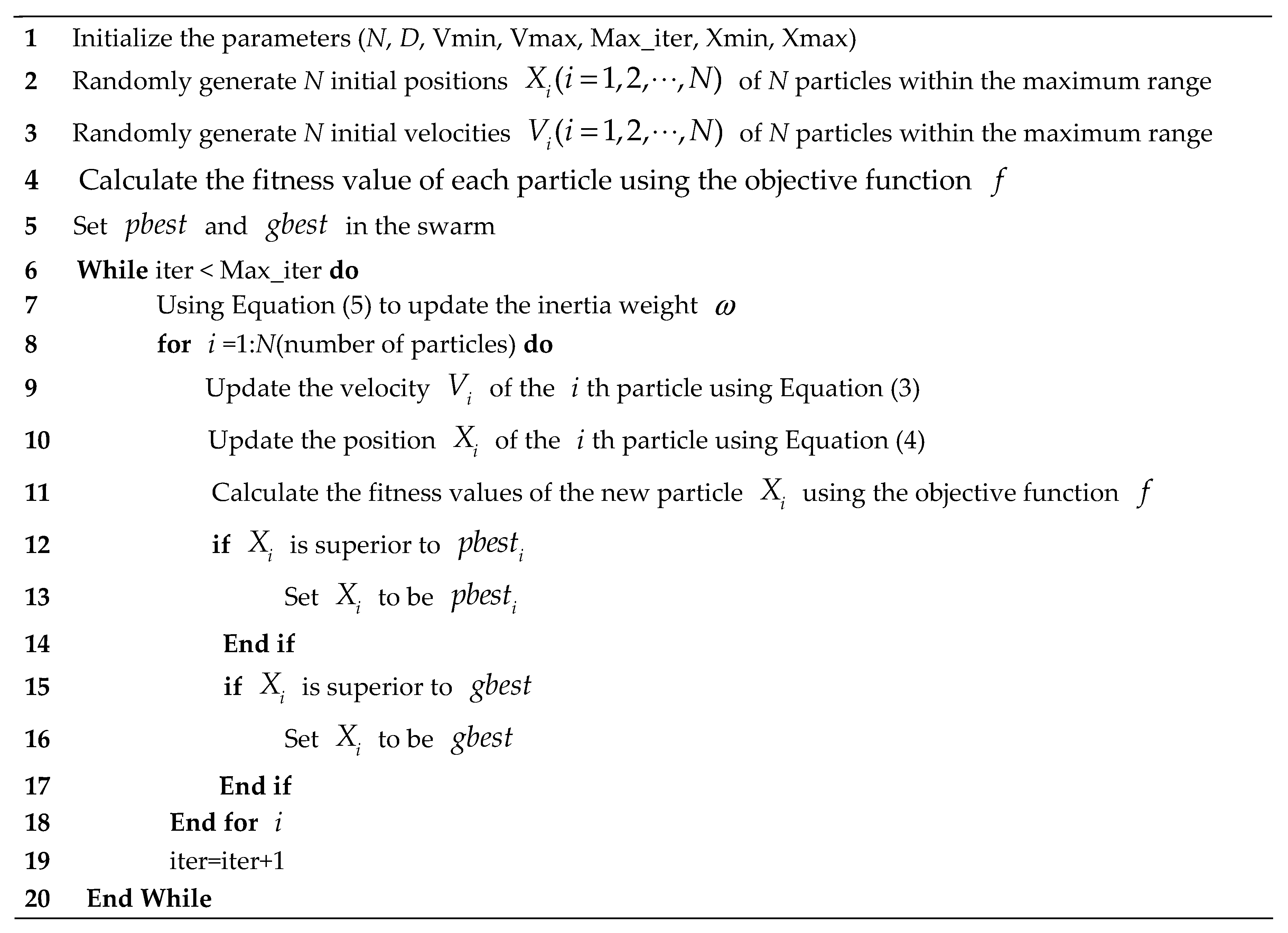
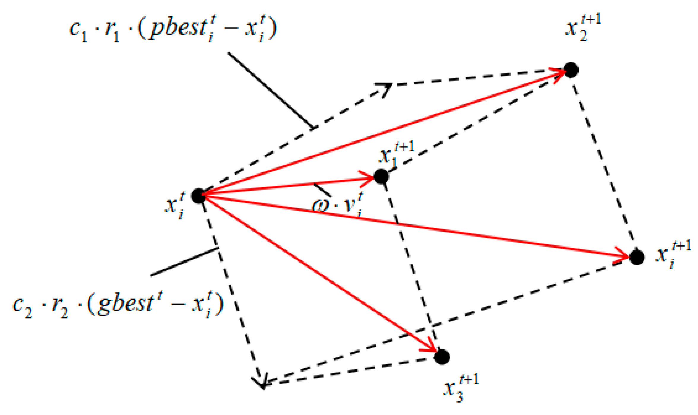
2. Related Theory about PSO

PSO is a kind of swarm intelligence optimization algorithm, which is derived from the study of bird swarm predation behavior. Each particle in the particle swarm represents a possible solution to a problem. Through the simple behavior of individual particles and the interaction of information within the group, the intelligence of solving problems is achieved.
PSO is a population-based search algorithm. An individual in the bird swarm is abstracted into a particle. Each particle searches for the optimal solution in the search space separately. The optimal solution that each particle can currently search for is recorded as the current individual optimal value, and then the individual optimal value is shared with other particles in the entire particle swarm. The optimal individual extreme value is found as the current global maximum of the whole particle swarm. All particles in the particle swarm continually update their positions and speeds based on the current individual extremes found by themselves and the current global optimal solution shared by the entire particle swarm. The particle will gradually approach the optimal position and finally find the global optimum during the iterative process.
When searching in D-dimensional target search space, each particle has two parameters, position and velocity. The position of the i th particle is represented as x i = ( x i 1 , x i 2 , , x i D ) , i = ( 1 , 2 , , N ) , where N is the number of population. The velocity of the i th particle is represented as v i = ( v i 1 , v i 2 , , v i D ) , i = ( 1 , 2 , , N ) . The velocity and position of the particles are iterated according to the following iterative equations:
v i ( t + 1 ) = v i t + c 1 r 1 ( p b e s t i t x i t ) + c 2 r 2 ( g b e s t t x i t )
x i ( t + 1 ) = x i t + v i ( t + 1 )
x i t indicates the position of the t th iteration of the i th particle. v i t denotes the speed of the t th iteration of the i th particle. c 1 and c 2 are two positive constants, generally c 1 = c 2 = 2 ; r 1 and r 2 are random numbers in the interval [0, 1]. Each particle is evaluated for fitness value f ( x i ) by objective function f . Each particle position represents a solution to the problem, which has a fitness value f ( x i ) , given by the objective function f . During each iteration process, the particles memorize the position with the best fitness value by comparing the fitness value of each position and update p b e s t , g b e s t . p b e s t i t is the current individual optimal position of the particle and g b e s t t is the current global optimal position of the entire particle swarm. Self-cognition component term c 1 r 1 ( p b e s t i t x i t ) pushes the particles to move toward their own best positions found so far. Social cognitive component term c 2 r 2 ( g b e s t t x i t ) encourages the particles to move toward the global best position found currently. v i [ v max , v max ] , and v max is a constant. v max often set to four in practice [33]. When the particle velocity exceeds the interval, let the particle velocity v i be equal to the upper or lower bound of the interval ( v max or v max ) so that the particle velocity is controlled within a reasonable range. Equations (1) and (2) are called the basic PSO algorithm.
In [34] Shi and Eberhart introduced inertial weight ω into the memory term in Equation (1) and found that it can balance the global search ability and local search ability better. The improved iterative equations are formulated as follows:
v i ( t + 1 ) = ω v i t + c 1 r 1 ( p b e s t i t x i t ) + c 2 r 2 ( g b e s t t x i t )
x i ( t + 1 ) = x i t + v i ( t + 1 )
where ω is a linear decreasing weight strategy defined as follows:
ω = ω max M j M max ( ω max ω min )
where ω min and ω max are the initial and final values of the inertial weight, respectively, M j is the current iteration number and M max is the maximum iteration number.
Since the inertial weight ω improves the performance significantly, scholars take it as the standard PSO algorithm, which has become the basis of the current research and improvement of PSO. The pseudo-code of the standard PSO algorithm is shown in Figure 1. Inspired by this linear decreasing ω , some articles have proposed different strategies on inertial weight [28,35].

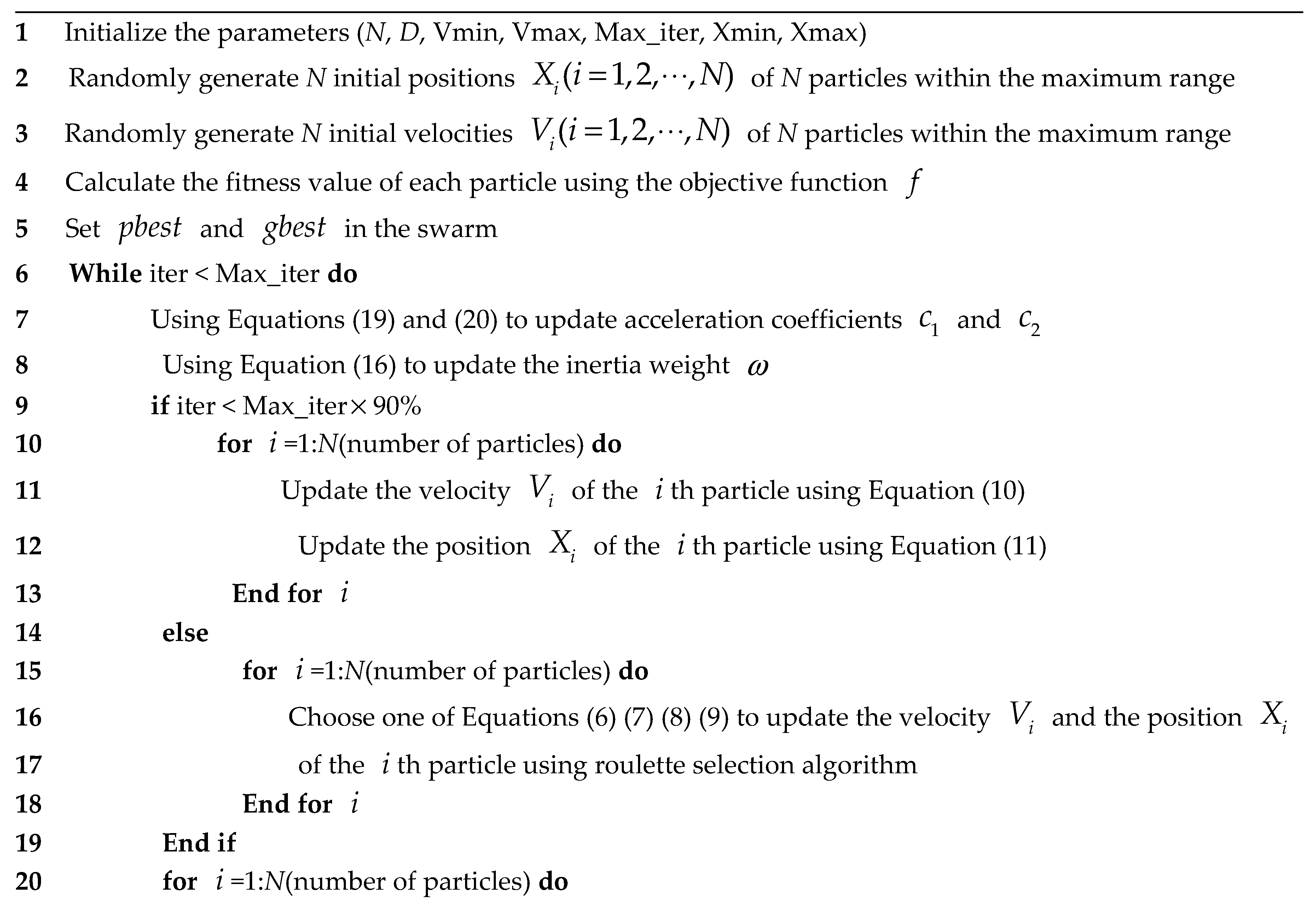
3. Hybrid Multi-Step Probability Selection Particle Swarm Optimization with Sine Chaotic Inertial Weight and Symmetric Tangent Chaotic Acceleration Coefficients (MPSPSO-ST)

The PSO algorithm currently has shown great effectiveness on various optimization problems, but it still has a drawback as lacking diversity in the search process. Due to premature convergence, the search is prone to stagnate and fall into local optimal solutions [36,37]. Based on the in-depth study of PSO, this paper proposes three modifications to improve the performance of PSO.

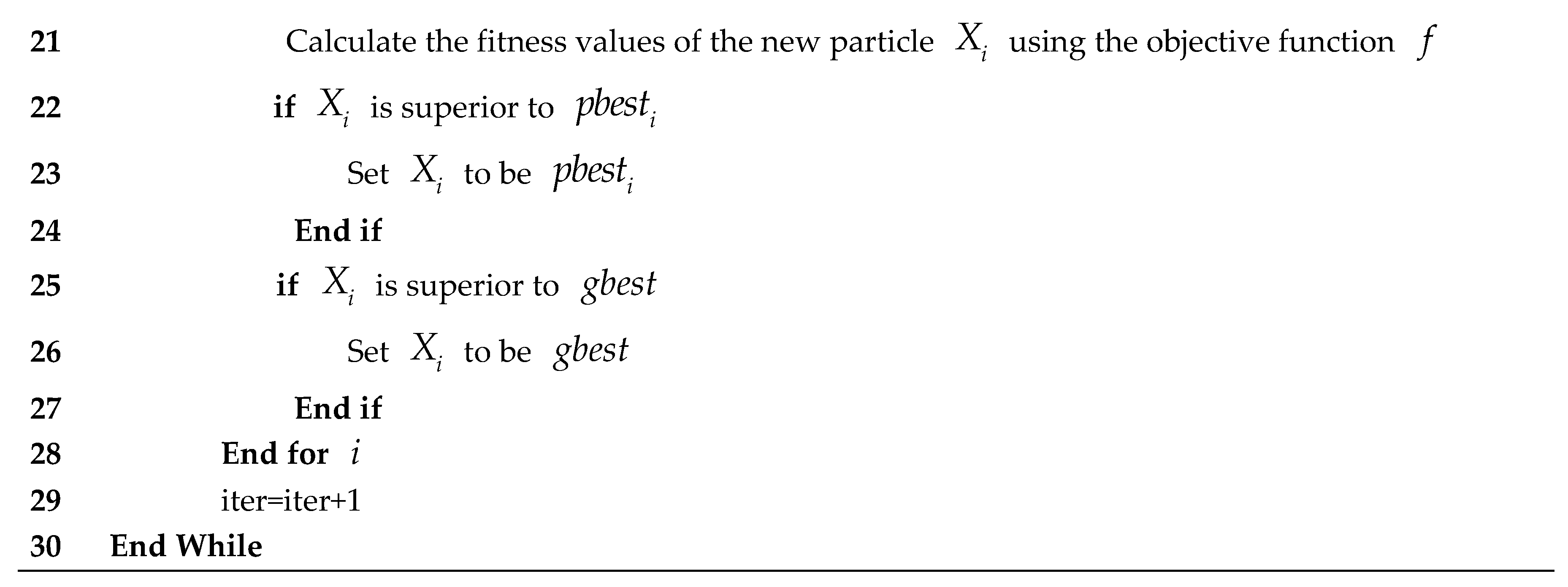
3.1. Hybrid Multi-Step Probability Selection Particle Swarm Optimization (MPSPSO)
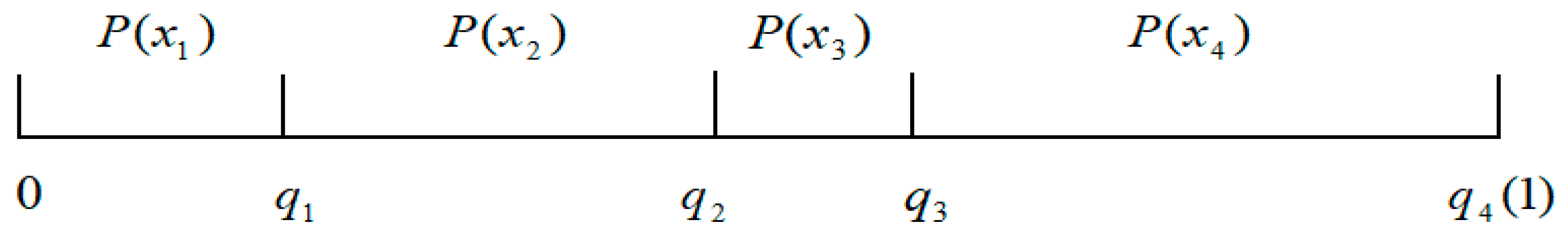
According to Equation (3), the particle velocity updated in the PSO algorithm is determined by three terms: inertia term v i t , self-cognition component term c 1 r 1 ( p b e s t i t x i t ) and social cognitive component term c 2 r 2 ( g b e s t t x i t ) . Inspired by human behavior, when humans do things, they sometimes perform habitually (the velocity update only includes inertia term v i t , as shown in Equation (6)), sometimes they sum up their own experience (the velocity update includes inertia term v i t and self-cognition component term c 1 r 1 ( p b e s t i t x i t ) , as shown in Equation (7)), and sometimes they summarize all the information and then do things (the basic PSO algorithm is this way, as shown in Equation (1)) [38].
Previous studies have shown that the length and direction of v i t are coupled with p b e s t i t and g b e s t t , resulting in a slow update of p b e s t i t [39]. Gao et al. [38] proposed a variant named PSO-MP to decompose the single-step velocity update formula in the standard PSO into the three-steps update and then choose the best one. This method that updating step-by-step first and then selecting the optimal value to update can achieve decoupling of v i t , p b e s t i t and g b e s t t , respectively. Thereby, the search ability of this algorithm is enhanced.
In order to increase the diversity and randomness of the particle population, this paper proposes a PSO variant using hybrid multi-step probability selection, namely MPSPSO. The main idea of this variant is to decompose the single-step velocity update formula in the standard PSO into four velocity update formulas. In the early iterations, we directly select the one with the best fitness value of four velocity update formulas. While in the later iterations, we probabilistically select one of the four velocity update formulas using the roulette wheel selection mechanism according to the fitness value. Finally, the optimal solution is obtained. This algorithm can not only achieve the decoupling of v i t , p b e s t i t and g b e s t t but also enhance the randomness and diversity of optimization, thereby effectively avoiding falling into local optimums, so that it can improve the search accuracy and efficiency. The detailed introduction about MPSPSO is presented as follows.
1. Calculate the particle velocity and position by Equations (3) and (4), where x i t + 1 is the vector sum with x i t , ω v i t , c 1 r 1 ( p b e s t i t x i t ) and c 2 r 2 ( g b e s t t x i t ) , as shown in Figure 2.
As can be seen from Figure 2, in the standard PSO, only x i t and x i t + 1 are used to update the particle position. x 1 t + 1 , x 2 t + 1 and x 3 t + 1 are used as temporary points only for the generation of x i t + 1 . These three points may be better than others, but they are ignored. Therefore, the velocity update Equation (3) is divided into four steps in this paper, and three temporary points are iterative objects which can be selected. The equations are described as follows:
v 1 t + 1 = ω v i t , x 1 t + 1 = x i t + v 1 t + 1
v 2 t + 1 = v 1 t + 1 + c 1 r 1 ( p b e s t i t x i t ) , x 2 t + 1 = x i t + v 2 t + 1
v 3 t + 1 = v 1 t + 1 + c 2 r 2 ( g b e s t t x i t ) , x 3 t + 1 = x i t + v 3 t + 1
v 4 t + 1 = v 1 t + 1 + c 1 r 1 ( p b e s t i t x i t ) + c 2 r 2 ( g b e s t t x i t ) , x 4 t + 1 = x i t + v 4 t + 1
2. If iteration < 0.9 × t max ( t max is the maximum iteration number), choose the position with the best fitness given by the objective function f (in this paper, we all solve min f ( x ) problem, so the smaller f ( x ) is, the better the fitness is) among the above equations as the final position x i t + 1 . The corresponding velocity is taken as the final velocity v i t + 1 .
The process is described as follows:
v i t + 1 = { v 1 t + 1 , i f min { f ( x 1 t + 1 ) , f ( x 2 t + 1 ) , f ( x 3 t + 1 ) , f ( x 4 t + 1 ) } = f ( x 1 t + 1 ) v 2 t + 1 , i f min { f ( x 1 t + 1 ) , f ( x 2 t + 1 ) , f ( x 3 t + 1 ) , f ( x 4 t + 1 ) } = f ( x 2 t + 1 ) v 3 t + 1 , i f min { f ( x 1 t + 1 ) , f ( x 2 t + 1 ) , f ( x 3 t + 1 ) , f ( x 4 t + 1 ) } = f ( x 3 t + 1 ) v 4 t + 1 , o t h e r w i s e
x i t + 1 = { x 1 t + 1 , i f min { f ( x 1 t + 1 ) , f ( x 2 t + 1 ) , f ( x 3 t + 1 ) , f ( x 4 t + 1 ) } = f ( x 1 t + 1 ) x 2 t + 1 i f min { f ( x 1 t + 1 ) , f ( x 2 t + 1 ) , f ( x 3 t + 1 ) , f ( x 4 t + 1 ) } = f ( x 2 t + 1 ) x 3 t + 1 i f min { f ( x 1 t + 1 ) , f ( x 2 t + 1 ) , f ( x 3 t + 1 ) , f ( x 4 t + 1 ) } = f ( x 3 t + 1 ) x 4 t + 1 o t h e r w i s e
The rationality and effectiveness of this step-by-step process are reflected in the refinement of the particle search trajectory. Firstly, the particles move by Equation (6) according to the speed and inertia of the previous step. If the search direction in the previous step is a direction that is closer to the best solution, then this position may be a better point. On the basis of x 1 t + 1 , move along the individual extreme value direction to x 2 t + 1 by Equation (7) to refine the local search; move to x 3 t + 1 along the global extreme value direction by Equation (8) to refine the global search; or comprehensively considering the individual extreme value and the global extreme value, move to x 4 t + 1 along the individual extreme value direction and the global extreme value direction by Equation (9) as the standard PSO. Such a step-by-step search operation can take the temporary points that were initially ignored as optional objects and achieve greater use of potential information so that the algorithm has multi-selected opportunities to find the optimal solution more efficiently.
3. After iterating to 90% of t max , according to the fitness of the four positions from Equations (6)–(9), given by the objective function f , we probabilistically select one of the four positions as the update particle position x i t + 1 of this generation using a roulette wheel selection mechanism. The particle velocity corresponding to this position is taken as the update particle velocity v i t + 1 . Roulette wheel selection [40] is widely used in improving various population-based algorithms such as GA [41] DE [42] which all achieve satisfactory results. Inspired by this, we propose the above idea.
Roulette wheel selection mechanism, also known as a proportional selection method, the basic idea of which is that the probability of an individual being selected is proportional to its fitness, that is, the size of the objective function value. The smaller the objective function value of the particle position is, the better the particle fitness is, the higher the probability of being selected is. The specific operations are as follows:
  • Calculate the objective function value f ( i = 1 , 2 , 3 , 4 ) of each of the four particle positions.
  • Due to it that the smaller f ( x ) is, the better the fitness of the position is, so the probability of being selected should be inversely proportional to the function value of the position. From this, the probability of each position being selected is calculated as follows:
    P ( x i ) = 1 f ( x i ) j = 1 4 f ( x j )
  • Calculate the cumulative probability of each position:
    q i = j = 1 i P ( x j )
The cumulative probability diagram is in Figure 3 as follows:
  • Randomly generate a uniformly distributed random number r in the interval [0, 1].
  • When r satisfies r < q 1 , select position x 1 t + 1 ; when r satisfies q k 1 < r q k , select position x k t + 1 .
After iterating to 90% of t max , the reason for using the roulette wheel selection mechanism is that the whole swarm are now close to the global optimum, but the swarm diversity in the later iterations is poor, and the point with the best fitness in this generation may not always approach the best solution quickly after iterative calculations, so the roulette wheel selection mechanism is used at the later stage of the iteration to select the final update point x i t + 1 . Possibility of selecting good particle positions for this generation is high but not absolutely and other particle positions may also be selected, which makes the choice of search direction more diverse. This operation enriches the swarm diversity and ensures that the ability to jump out of local extreme value is effectively modified.
Similar to the next iteration, each particle will modify its speed and position within each iteration until the optimal solution is found or all iterations are terminated. MPSPSO successfully avoids premature convergence and greatly increases the possibility of finding the optimal solution.

3.2. Sine Chaotic Inertia Weight ω

The inertia weight plays a vital role in the convergence behavior of PSO [34,43]. Chaos is a nonlinear dynamic phenomenon, which has regularity, randomness and ergodicity. Due to these characteristics, chaos has become a popular optimization method today. Optimizing the search by chaos mechanism is superior to stochastic search [44,45]. It has the ability not to repeatedly go through all states in a certain range, which can meet the needs of ω for different functions to the greatest extent [46]. The authors of [47] compared 15 classic methods of inertial weight, and the result indicates that chaotic inertial weight is the best strategy to improve accuracy.
Previous research has shown that the sine function plays a great role in the adjustment of ω [48,49]. Combining the sine function and chaos mechanism, this paper uses a sine iterator to directly generate the sequence to achieve the sine chaotic inertial weight.
A sine iterator is a type of chaotic sequence generator. Mathematically, its basic form is as follows:
X n + 1 = a x n 2 sin ( π x n )
When a = 2.3 , X 0 = 0.7 , its simple form is as follows:
X n + 1 = sin ( π x n )
It generates chaotic sequences in (0, 1).
Therefore, this paper proposes the following update form of ω :
ω t + 1 = ϕ × sin ( π ω t ) + τ
The initial value ω 1 is an arbitrary number in [0, 1], and ϕ , τ are constants.
In this paper, we take ϕ = 0.9 , τ = 0 . With the progress of the iterative process, ω can traverse almost all values in the interval of [0.2, 0.9] approximately. The proposal of sine chaotic inertial weight can enhance the global exploration of the algorithm and strengthen the ability of avoiding local optimum.

3.3. Symmetric Tangent Chaotic Acceleration Coefficients c 1 , c 2

The cognitive component c 1 and social component c 2 are very important for the algorithm to find the optimal solution accurately and efficiently. Usually, the cognitive component and social component are given equal weight c 1 = c 2 = 2 . With a large cognitive component and a small social component at the beginning, particles are allowed to move around the search space during the early stages. On the other hand, a small cognitive component and a large social component allow the particles to converge to the global optimum in the latter part of the optimization process [50]. Logistic mapping in the chaos mechanism has attracted much attention owing to better optimization performance, such as randomness and ergodicity. Based on the above two points, this paper proposes symmetric tangent chaotic acceleration coefficients.
The formula of Logistic mapping is z = μ × z × ( 1 z ) , and chaos performance is best when μ = 4 . This paper firstly proposes the symmetric tangent acceleration coefficient, and then introduces the chaotic term. The equations of the symmetric tangent acceleration coefficients are as follows:
c 1 = × m 2 × tan [ π 8 × ( 1 + m 2 ) ] + θ
c 2 = × ( 1 m ) 2 × tan [ π 8 × ( 1 + ( 1 m ) 2 ) ] + θ
where m = t t max , t is the current number of iterations, t max is the maximum number of iteration, and , θ are constants.
Then add chaotic terms to Equations (17) and (18): firstly, take a random number in (0,1), then generate the Logistic mapping sequence. We propose the symmetric tangent chaotic acceleration coefficients, which are defined by Equations (19) and (20).
c 1 = × m 2 × tan [ π 8 × ( 1 + m 2 ) ] + θ + ρ × z
c 2 = × ( 1 m ) 2 × tan [ π 8 × ( 1 + ( 1 m ) 2 ) ] + θ + ρ × z
where ρ is a constant.
This paper takes = 0.2 , θ = 1.5 and ρ = 0.1 . The proposal of the symmetric tangent acceleration factor enables the algorithm to balance the global search in the early stage of iteration and the local search in the later stage of iteration better. Meanwhile, the proposal of chaotic terms makes the acceleration coefficients have chaotic characteristics while maintaining the original change trend.
Summarizing the above description, the pseudo-code of MPSPSO-ST proposed in this paper is shown in Figure 4:

4. Experimental Results and Discussion

In this study, we used 20 well-known multi-dimensional classical benchmark functions, i.e., objective function f , to perform a large number of experiments to evaluate the performance of MPSPSO-ST proposed in this paper. These test functions were adopted by extensive literature [51,52]. We conducted two groups of experiments: in the first group, we compared the search performance of MPSPSO-ST with standard PSO, basic PSO, MPSPSO. In the second group, we compared MPSPSO-ST with three PSO variants (chaos particle swarm optimization (CPSO), particle swarm optimization with the nonlinear dynamic acceleration coefficients (PSO-NDAC), adaptive inertia weight and acceleration coefficients PSO (AIWCPSO)) and three well-known similar optimization algorithms (DE, MFO, SCA).
The Appendix A lists 20 classic benchmark functions adopted for this experiment to test the performance of MPSPSO-ST. These test functions are divided into two types. The first type contains eight unimodal functions and the second type contains 12 multimodal functions. There are many well-known functions, like f 10 (Michalewicz), f 11 (Griewank), f 13 (levy) and f 19 (Zakharov). f 10 (Michalewicz) has d! local minima. The parameter m defines the steepness of the valleys and ridges and a larger m leads to a more difficult search. f 11 (Griewank) has many widespread local minima, which causes more difficulties in searching for the global optimum. f 13 (levy) and f 19 (Zakharov) are both widely used in the optimization field because they are classical. Dim, Range and fmin represent the space dimensions of solution, the range of function variation and the minimum value of the function, that is, the optimal solutions, respectively.

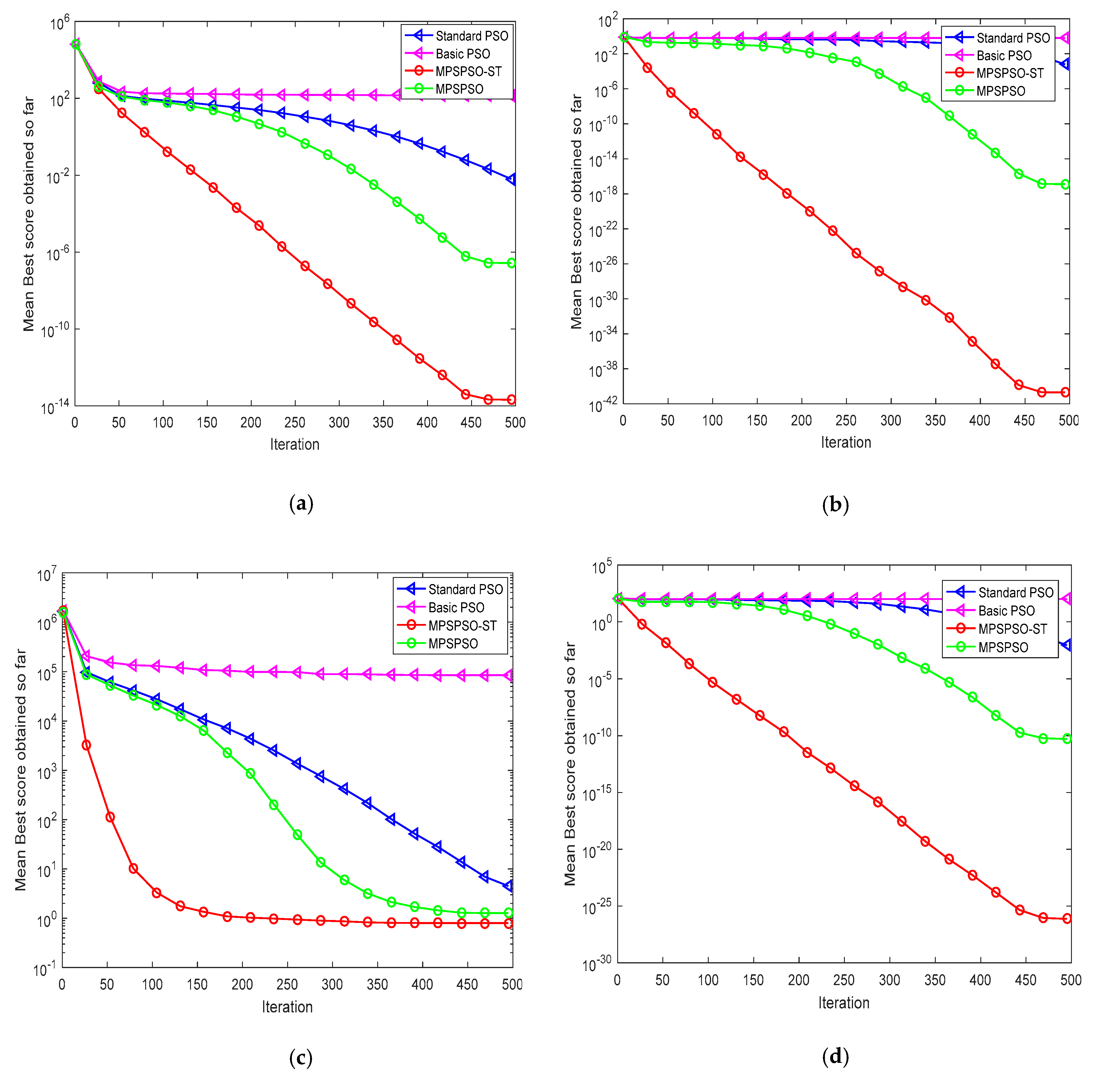
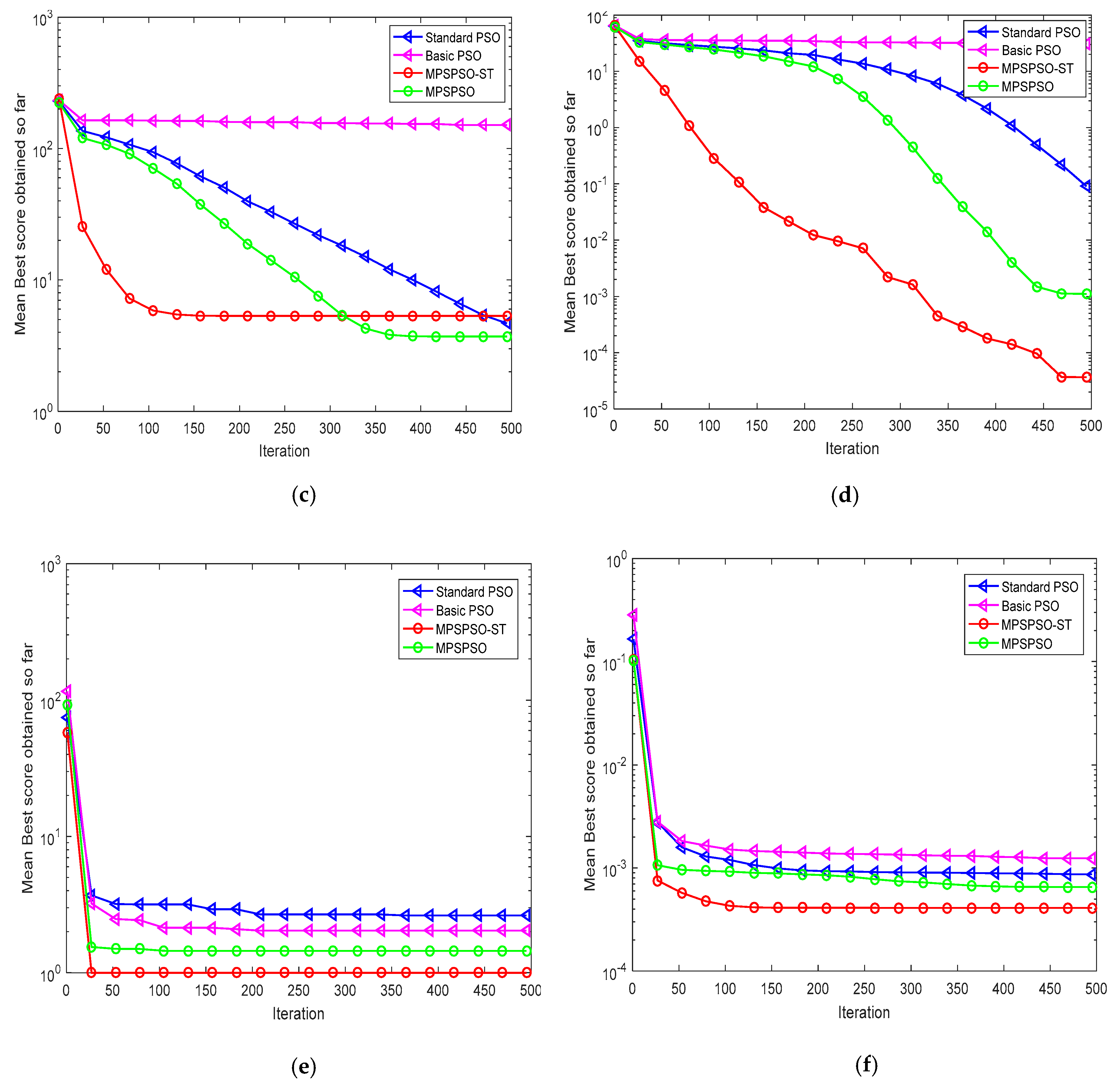
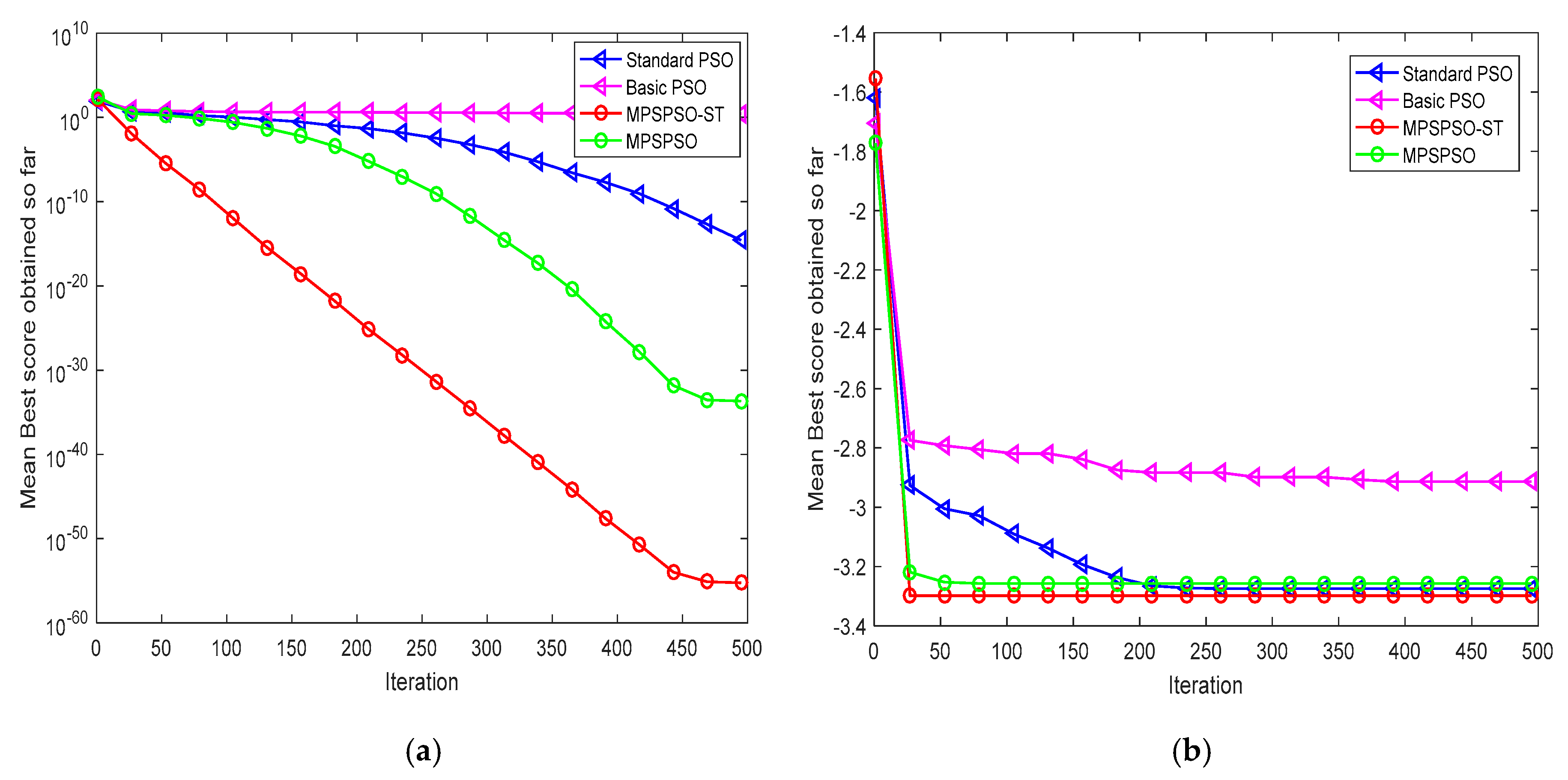
4.1. Comparison of MPSPSO-ST with Standard PSO, Basic PSO and MPSPSO

The parameter settings for MPSPSO-ST, Standard PSO, Basic PSO and MPSPSO are shown in Table 1. The experimental results obtained by testing the 20 benchmark functions in the Appendix A are shown in Table 2. The convergence diagrams of the four algorithms are shown in Figure 5, Figure 6 and Figure 7. The values in the diagrams are the mean best results of 20 runs of the whole swarm so far.
Figure 5 clearly shows that compared to the other three algorithms, MPSPSO-ST has very prominent advantages, which offers the fastest convergence speed and the strongest optimization accuracy. From Figure 6a,d,e,f, we observe that for multimodal functions f 10 , f 15 , f 17 , f 18 , MPSPSO-ST owns faster convergence speed and better optimization performance compared with the other three algorithms, especially these advantages are more outstanding for f 10 , f 15 , f 17 . However, for multimodal functions f 11 , f 13 in Figure 6b,c, the performance of MPSPSO-ST is not as good as that of MPSPSO and Standard PSO. Nevertheless, MPSPSO-ST can maintain a faster convergence rate when the final optimization results of MPSPSO-ST and MPSPSO, Standard PSO are quite close. As seen from Figure 7, the convergence speed and global search capability of MPSPSO-ST are the most competitive for multimodal functions f 19 , f 20 .
The information in Table 2 can reflect the above conclusions more specifically and accurately. The indicators in Table 2 are the best values (the best), the worst value (the worst), mean value (mean), standard deviation (S.D.) of MPSPSO-ST and Standard PSO and Basic PSO, MPSPSO in 20 independent running experiments. Among all unimodal functions f 1 ~ f 8 and multimodal functions f 9 , f 10 , f 15 , f 16 , f 17 , f 18 , f 19 and f 20 , MPSPSO-ST overtakes all other methods in terms of convergence rate and optimization accuracy. Especially for multimodal functions f 16 and f 17 , MPSPSO-ST can all reach the theoretical optimal value in a few iterations and the S.D. of MPSPSO-ST can reach 0. It means that MPSPSO-ST can achieve theoretical optimal value in each of 20 independent experiments, which shows MPSPSO-ST has steadier search ability than the other three algorithms during the search process. For multimodal functions f 11 , f 12 and f 14 , the optimization performance of MPSPSO-ST is not optimal, but it is the best at The best, indicating that MPSPSO-ST has obtained the best optimization results in the optimization of these test functions but the overall has not been maintained. Meanwhile, it can be seen that the standard deviation of MPSPSO-ST is smaller than the other three algorithms in a majority of test functions, illustrating that it has stronger robustness and stability.
As seen from Table 2, Figure 5, Figure 6 and Figure 7, we can conclude that the proposed MPSPSO-ST owns better optimization capability compared with Standard PSO, Basic PSO and MPSPSO, which indicates that MPSPSO-ST has excellent ability in solving numerical optimization problems.

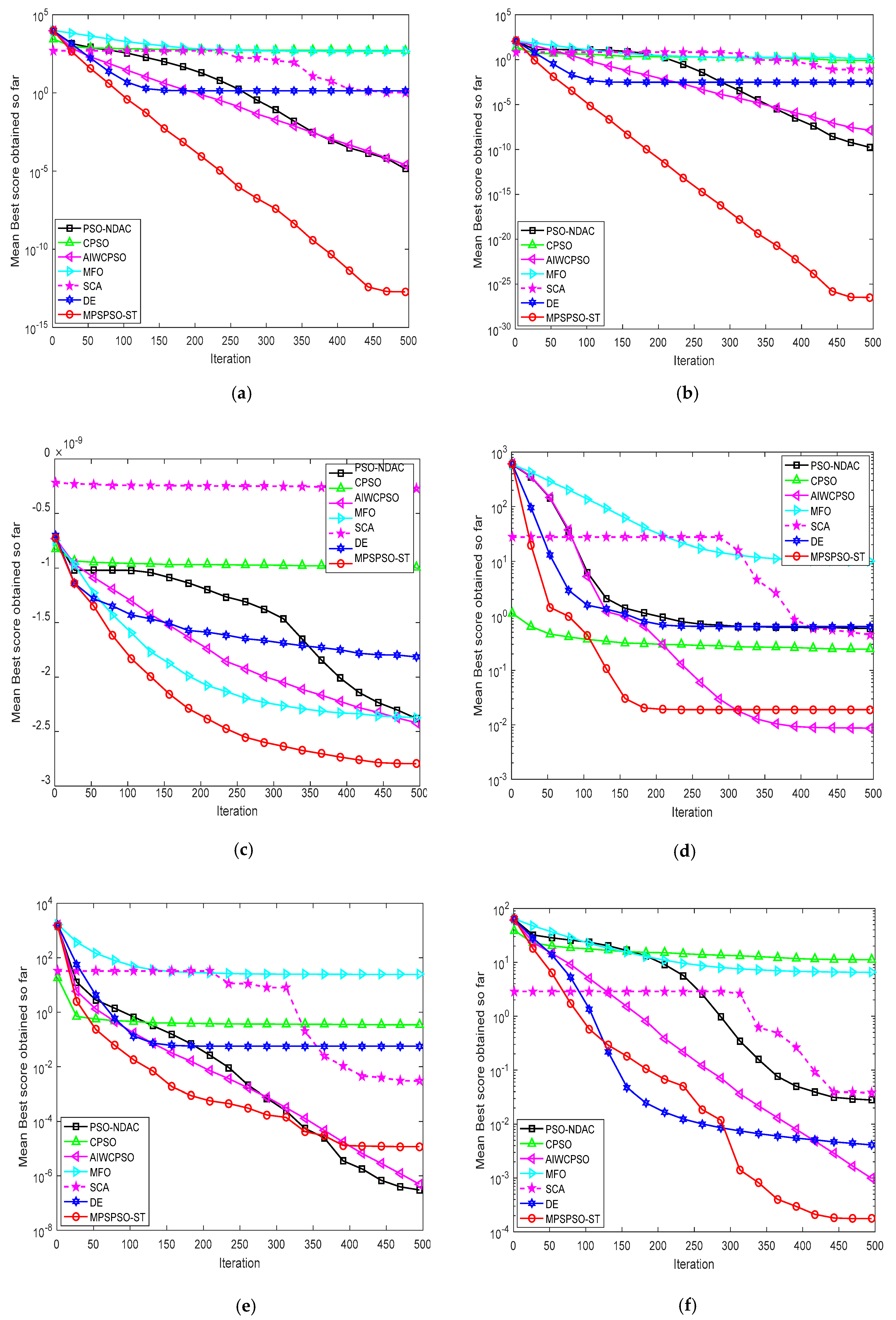
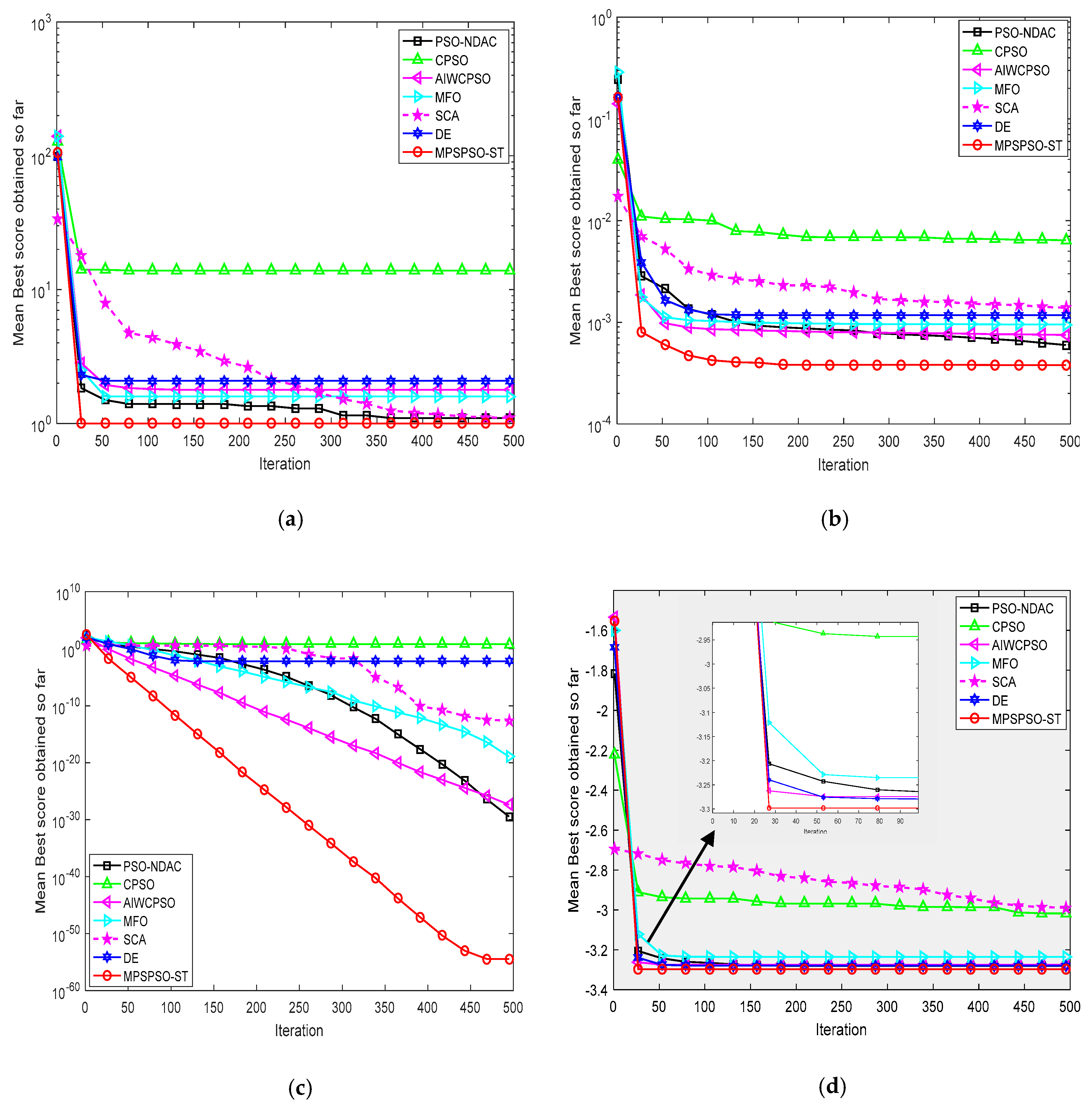
4.2. Comparison of MPSPSO-ST with CPSO, PSO-NDAC, AIWCPSO, DE, MFO and SCA

In this section, we have designed comparisons of MPSPSO-ST with several classic improved PSO variants (chaos particle swarm optimization (CPSO) [53] particle swarm optimization with the nonlinear dynamic acceleration coefficients (PSO-NDAC) [32] AIWCPSO [54]) and other well-known classic optimization algorithms (differential evolution algorithm (DE), moth-flame optimization algorithm (MFO) and sine cosine algorithm (SCA)). CPSO realizes chaotic searching on the current global best individual using chaos mechanism. PSO-NDAC proposes the nonlinear dynamic acceleration coefficients to add to PSO. AIWCPSO designs an inertia weight strategy that the adaptive inertia weight is adjusted according to the updated particles of the previous generation. DE is a group-based adaptive global optimization algorithm, which belongs to an evolutionary algorithm. MFO is a swarm intelligence optimization algorithm, the main inspiration of which is the navigation method of moths in nature called transverse orientation. SCA creates multiple initial random candidate solutions and requires them to fluctuate outwards or towards the best solution based on sine and cosine functions. The parameter settings for each algorithm are shown in Table 3.
The experimental results obtained by the test functions listed in the Appendix A are shown in Table 4. The convergence diagrams of the seven algorithms are shown in Figure 8, Figure 9 and Figure 10, and the values in the diagrams are the mean best results in 20 runs in the whole swarm so far.
As seen from Figure 8, MPSPSO-ST has an undeniable advantage in terms of convergence rate and optimization accuracy for unimodal functions f 1 , f 3 , f 4 , f 6 compared with the other six algorithms. Figure 9a–c,f show that MPSPSO-ST also has the best convergence rate and solution accuracy for multimodal functions f 7 , f 8 , f 10 , f 15 . Through Figure 9d,e, we find that the search performance of MPSPSO-ST is not optimal for multimodal functions f 11 , f 14 . For multimodal function f 11 , MPSPSO-ST has the best performance except for AIWCPSO. Furthermore, in the case where the optimization effect of MPSPSO-ST is very close to the optimization effect of AIWCPSO, MPSPSO-ST has a faster convergence speed to the global optimal solution than AIWCPSO. For multimodal functions f 17 , f 18 , f 19 , f 20 in Figure 10, MPSPSO-ST outperforms the other six methods.
As shown in Table 4, for multimodal functions f 11 and f 12 , MPSPSO-ST is not the best but The best it can find is the greatest compared to other algorithms, which shows that MPSPSO -ST has the ability to find the best results in 20 independent experiments but it has not been maintained in general. Besides, for multimodal functions f 16 , f 17 , the theoretical optimal value can be successfully found each time by MPSPSO-ST in 20 independent experiments, which indicates that the search performance of MPSPSO-ST is very stable. Therefore, we can see that MPSPSO-ST has prominent advantages in robustness and stability.
Combining Table 4 and Figure 8, Figure 9 and Figure 10, among the 20 classical benchmark functions f 1 ~ f 20 , referring to two indicators, mean (mean) and standard deviation (S.D.) in Table 4, MPSPSO-ST is significantly superior to the other six algorithms in searching better global optimal value for these 16 test functions f 1 ~ f 10 , f 15 ~ f 20 . In addition, although the final optimization result of MPSPSO-ST is inferior to AIWCPSO for multimodal function f 11 , it is extremely close to AIWCPSO in terms of optimization effect and has the fastest convergence speed, and its convergence accuracy is better than the five other algorithms except for AIWCPSO, so MPSPSO-ST is used as the most efficient optimization algorithm. For multimodal functions f 11 , f 14 , AIWCPSO shows the best performance. For multimodal function f 12 , PSO-NDAC has the best performance. The performance of AIWCPSO and PSO-NDAC is similar in other test functions, second only to MPSPSO-ST, so AIWCPSO and PSO-NDAC are tied as the second most effective optimization algorithm. DE is listed as the third most effective algorithm, achieving the best solution on multimodal function f 13 . Although SCA has not got the best solution in the optimization of any test function, from the indicator The best in Table 4, SCA has found better optimal values than other algorithms in 20 independent experiments for unimodal function f 7 and multimodal function f 14 , but the lack of maintenance leads to a general mean. So SCA is listed as the fourth most influential optimization algorithm. For CPSO and MFO, they are unable to find a better global optimal solution than all other algorithms in all test functions.
To sum up, it can be concluded that MPSPSO-ST offers superior overall performance among all seven algorithms, followed by AIWCPSO and PSO- NDAC, then DE, then SCA, and finally CPSO and MFO.
In general, each category used to assess a specified behavior in the optimization algorithm. The unimodal functions are used to assess the convergence rate of the algorithm since they contain a single extreme solution in the search domain ( f 1 ~ f 8 ). Meanwhile, the multimodal functions are used to evaluate the ability of the algorithm to avoid the local point and reach to global solution since they contain more than an extreme solution ( f 9 ~ f 20 ) 52In the above two experiment sections, among 20 test functions applied in this paper, MPSPSO-ST is significantly superior to other comparison algorithms for all unimodal functions and most multimodal functions, which reflects that MPSPSO-ST has an excellent convergence speed and the ability to get rid of local extreme values.

5. Conclusions

In this paper, we propose the MPSPSO-ST algorithm, which can facilitate the algorithm performance of the traditional PSO. Firstly, we propose a hybrid multi-step probability selection update mechanism, i.e., the MPSPSO algorithm. Secondly, based on the MPSPSO algorithm, in order to achieve a good balance between exploration and exploitation to optimize the performance of the algorithm, we design the sine chaotic inertial weight and symmetric tangent chaotic acceleration coefficients, which are integrated into the MPSPSO-ST algorithm. Finally, to appraise the effectiveness of the MPSPSO-ST algorithm, we conduct extensive experiments with 20 classic benchmark functions and the experiments consisted of two groups. The first group of experiments is the comparisons of MPSPSO-ST with the Standard PSO, Basic PSO and MPSPSO. The experimental results show that the hybrid multi-step probability selection update mechanism proposed in this paper is very effective. The sine chaotic inertial weight and the symmetric tangent chaotic acceleration coefficients proposed on this basis can effectively maintain swarm diversity in the search process, which enhances the performance of MPSPSO-ST significantly. The second group of experiments is the comparisons of the MPSPSO-ST algorithm with three classical improved PSO variants (CPSO, PSO-NDAC, AIWCPSO) and three well-known classic optimization algorithms (DE, MFO, SCA). The experimental results show that the MPSPSO-ST algorithm surpasses all other six algorithms obviously on the majority of the classic benchmark functions, with faster convergence speed, higher optimization accuracy, and greater stability robustness, which is successful in solving numerical optimization tasks. MPSPSO-ST has the basic characteristics of PSO, simple, easy to realize and other advantages while taking the search accuracy and search efficiency into account. It can further avoid premature convergence to a certain extent. Besides, MPSPSO-ST does not introduce any new parameters, making it more versatile and easier to operate and realize. Indeed, the proposed modification implies increasing complexity of the algorithm, but it is worthwhile in order to solve complex numerical optimization problems more efficiently.
Therefore, the MPSPSO-ST algorithm proposed in this paper is an excellent choice for solving complex numerical optimization problems. In the future, we will further develop the strategies of parameter tuning and study the application of the MPSPSO-ST algorithm in practical problems.

Author Contributions

Conceptualization, Y.D.; methodology, Y.D.; software, Y.D. and F.X.; formal analysis, F.X.; data curation, Y.D. and F.X.; writing—original draft preparation, Y.D.; writing—review and editing, Y.D. and F.X. All authors have read and agreed to the published version of the manuscript.

Funding

The authors have received no funding for this work.

Acknowledgments

The authors gratefully acknowledge the support of anonymous reviewers.

Conflicts of Interest

The authors declare that there are no conflicts of interest.

Appendix A

Table A1. The 20 multi-dimensional classical benchmark functions are given below.
IDTest FunctionDimRangefminType
f 1 f ( x ) = i = 1 n x i 2 30[−100, 100]0Unimodal
f 2 f ( x ) = i = 1 n i x i 4 + r a n d o m [ 0 , 1 ] 30[−1.28, 1.28]0Unimodal
f 3 f ( x ) = i = 1 n ( j = 1 i x j ) 2 30[−100, 100]0Unimodal
f 4 f ( x ) = i = 1 n | x i | i + 1 30[−1, 1]0Unimodal
f 5 f ( x ) = ( x 1 1 ) 2 + i = 2 n i ( 2 x i 2 x i 1 ) 2 30[−10, 10]0Unimodal
f 6 f ( x ) = i = 1 n ( [ x i + 0.5 ] ) 2 30[−100, 100]0Unimodal
f 7 f ( x ) = i = 1 n i x i 2 30[−10, 10]0Unimodal
f 8 f ( x ) = i = 1 n i x i 4 30[−1.28, 1.28]0Unimodal
f 9 f ( x ) = 1 cos ( 2 π i = 1 n x i 2 ) + 0.1 i = 1 n x i 2 30[−100, 100]0Multimodal
f 10 f ( x ) = i = 1 n sin ( x i ) ( sin ( i x i 2 π ) ) 2 m , m = 10 30[0, π ]−4.687Multimodal
f 11 f ( x ) = 1 4000 i = 1 n x i 2 i = 1 n cos ( x i i ) + 1 30[−600, 600]0Multimodal
f 12 f ( x ) = π n { 10 sin 2 ( π y 1 ) + i = 1 n 1 ( y i 1 ) 2 [ 1 + 10 sin 2 ( π y i + 1 ) ] + ( y n 1 ) 2 } + i = 1 n u ( x i , 10 , 100 , 4 ) , y i = 1 + x i + 1 4 u ( x i , a , k , m ) = { k ( x i a ) m , x i > a 0 , a x i a k ( x i a ) m , x i < a 30 [−50, 50] 0 Multimodal
f 13 f ( x ) = 0.1 sin 2 ( 3 π x 1 ) + i = 1 n 1 ( x i 1 ) 2 + sin 2 ( 3 π x i + 1 ) + ( x n 1 ) 2 ( 1 + sin 2 ( 3 π x n ) ) 30[−5, 5]0Multimodal
f 14 f ( x ) = i = 1 n ( 10 6 ) i 1 n 1 x i 2 30[−100, 100]0Multimodal
f 15 f ( x ) = i = 1 n | x i sin ( x i ) + 0.1 x i | 30[−10, 10]0Multimodal
f 16 f ( x ) = [ 1 + ( x 1 + x 2 + 1 ) 2 ( 19 14 x 1 + 3 x 1 2 14 x 2 + 6 x 1 x 2 + 3 x 2 2 ) ] × [ 30 + ( 2 x 1 3 x 2 ) × ( 18 32 x 1 + 12 x 1 2 + 48 x 2 36 x 1 x 2 + 27 x 2 2 ) ] 2 [−2, 2] 3 Multimodal
f 17 f ( x ) = ( 1 500 + j = 1 25 1 j + i = 1 2 ( x i a i j ) 6 ) 1 2 [−65.536, 65.536] 0.998 Multimodal
f 18 f ( x ) = i = 1 11 [ a i x 1 ( b i 2 + b i x 2 ) b i 2 + b i x 3 + x 4 ] 2 4[−5, 5]0Multimodal
f 19 f ( x ) = i = 1 n x i 2 + ( i = 1 n 0.5 i x i ) 2 + ( i = 1 n 0.5 i x i ) 4 6[−5, 10]0Multimodal
f 20 f ( x ) = i = 1 4 c i exp ( j = 1 6 a i j ( x j p i j ) 2 ) 6[0, 1]−3.32Multimodal

References

  1. Kennedy, J.; Eberhart, R. Particle swarm optimization. In Proceedings of the IEEE International Conference on Neural Networks, Perth, Australia, 27 November–1 December 1995; pp. 1942–1948. [Google Scholar]
  2. Mirjalili, S.; Mirjalili, S.M.; Lewis, A. Grey wolf optimizer. Adv. Eng. Softw. 2014, 69, 46–61. [Google Scholar] [CrossRef] [Green Version]
  3. Mirjalili, S.; Lewis, A. The whale optimization algorithm. Adv. Eng. Softw. 2016, 95, 51–67. [Google Scholar] [CrossRef]
  4. Das, S.; Mullick, S.S.; Suganthan, P.N. Recent advances in differential evolution—An updated survey. Swarm Evol. Comput. 2016, 27, 1–30. [Google Scholar] [CrossRef]
  5. Rashedi, E.; Nezamabadi-Pour, H.; Saryazdi, S. GSA: A gravitational search algorithm. Inf. Sci. 2009, 179, 2232–2248. [Google Scholar] [CrossRef]
  6. Mirjalili, S. Moth-flame optimization algorithm: A novel nature-inspired heuristic paradigm. Knowl. Based Syst. 2015, 89, 228–249. [Google Scholar] [CrossRef]
  7. Simon, D. Biogeography-based optimization. IEEE Trans. Evol. Comput. 2008, 12, 702–713. [Google Scholar] [CrossRef] [Green Version]
  8. Mirjalili, S. SCA: A sine cosine algorithm for solving optimization problems. Knowl. Based Syst. 2016, 96, 120–133. [Google Scholar] [CrossRef]
  9. Gandomi, A.H.; Alavi, A.H. Krill herd: A new bio-inspired optimization algorithm. Commun. Nonlinear Sci. 2012, 17, 4831–4845. [Google Scholar] [CrossRef]
  10. Ozturk, C.; Hancer, E.; Karaboga, D. A novel binary artificial bee colony algorithm based on genetic operators. Inf. Sci. 2015, 297, 154–170. [Google Scholar] [CrossRef]
  11. Mirjalili, S. The ant lion optimizer. Adv. Eng. Softw. 2015, 83, 80–98. [Google Scholar] [CrossRef]
  12. Jain, I.; Jain, V.K.; Jain, R. Correlation feature selection based improved-binary particle swarm optimization for gene selection and cancer classification. Appl. Soft Comput. 2018, 6, 203–215. [Google Scholar] [CrossRef]
  13. Zhang, H.; Lin, W.; Chen, A. Path planning for the mobile robot: A review. Symmetry 2018, 10, 450. [Google Scholar] [CrossRef] [Green Version]
  14. Phoemphon, S.; So-In, C.; Niyato, D.T. A hybrid model using fuzzy logic and an extreme learning machine with vector particle swarm optimization for wireless sensor network localization. Appl. Soft Comput. 2018, 65, 101–120. [Google Scholar] [CrossRef]
  15. Qin, T.C.; Zeng, S.K.; Guo, J.B.; Skaf, Z. State of health estimation of li-ion batteries with regeneration phenomena: A similar rest time-based prognostic framework. Symmetry 2017, 9, 4. [Google Scholar] [CrossRef] [Green Version]
  16. Wu, J.P.; Lin, B.L.; Wang, H.; Zhang, X.H.; Wang, Z.K. Optimizing the high-level maintenance planning problem of the electric multiple unit train using a modified particle swarm optimization algorithm. Symmetry 2018, 10, 349. [Google Scholar] [CrossRef] [Green Version]
  17. Wang, H.; Sun, H.; Li, C.H.; Rahnamayan, S.; Pan, J.S. Diversity enhanced particle swarm optimization with neighborhood search. Inf. Sci. 2013, 223, 119–135. [Google Scholar] [CrossRef]
  18. Joines, J.A.; Houck, C.R. On the use of non-stationary penalty functions to solve nonlinear constrained optimization problems with GA’s. In Proceedings of the First IEEE Conference on Evolutionary Computation, Orlando, FL, USA, 27–29 June 1994; pp. 579–584. [Google Scholar]
  19. Fogel, D.B. An Introduction to Simulated Evolutionary Optimization. IEEE Trans. Neur. Netw. 1994, 5, 3–14. [Google Scholar] [CrossRef] [Green Version]
  20. Liang, J.J.; Qin, A.K.; Suganthan, P.N.; Baskar, S. Comprehensive learning particle swarm optimizer for global optimization of multimodal functions. IEEE Trans. Evol. Comput. 2006, 10, 281–295. [Google Scholar] [CrossRef]
  21. Yang, J.; Zhu, H.; Wang, Y. An orthogonal multi-swarm cooperative PSO algorithm with a particle trajectory knowledge base. Symmetry 2017, 9, 15. [Google Scholar] [CrossRef] [Green Version]
  22. Jensi, R.; Jiji, G.W. An enhanced particle swarm optimization with levy flight for global optimization. Appl. Soft Comput. 2016, 43, 248–261. [Google Scholar] [CrossRef]
  23. Turgut, O.E. Hybrid chaotic quantum behaved particle swarm optimization algorithm for thermal design of plate fin heat exchangers. Appl. Math. Model. 2016, 40, 50–69. [Google Scholar] [CrossRef]
  24. Qin, J.; Liu, Y.; Grosvenor, R.; Lacan, F.; Jiang, Z.G. Deep learning-driven particle swarm optimisation for additive manufacturing energy optimisation. J. Clean. Prod. 2020, 245, 118702. [Google Scholar] [CrossRef]
  25. Shi, Y. Optimization of PID parameters of hydroelectric generator based on adaptive inertia weight PSO. In Proceedings of the IEEE 8th Joint International Information Technology and Artificial Intelligence Conference (ITAIC), Chongqing, China, 24–26 May 2019; pp. 1854–1857. [Google Scholar]
  26. Tian, D.; Zhao, X.; Shi, Z. Chaotic particle swarm optimization with sigmoid-based acceleration coefficients for numerical function optimization. Swarm Evol. Comput 2019, 51, 100573. [Google Scholar] [CrossRef]
  27. Arasomwan, M.A.; Adewumi, A.O. On adaptive chaotic inertia weights in particle swarm optimization. In Proceedings of the IEEE Symposium on Swarm Intelligence (SIS), Singapore, 16–19 April 2013; pp. 72–79. [Google Scholar]
  28. Taherkhani, M.; Safabakhsh, R. A novel stability-based adaptive inertia weight for particle swarm optimization. Appl. Soft Comput. 2016, 38, 281–295. [Google Scholar] [CrossRef]
  29. Zhang, C.S.; Ning, J.X.; Lu, S.A.; Ouyang, D.T.; Ding, T.A. A novel hybrid differential evolution and particle swarm optimization algorithm for unconstrained optimization. Oper. Res. Lett. 2009, 37, 117–122. [Google Scholar] [CrossRef]
  30. Garg, H. A hybrid PSO-GA algorithm for constrained optimization problems. Appl. Math. Comput. 2016, 274, 292–305. [Google Scholar] [CrossRef]
  31. Javidrad, F.; Nazari, M.; Javidrad, H.R. Optimum stacking sequence design of laminates using a hybrid PSO-SA method. Compos. Struct. 2018, 185, 607–618. [Google Scholar] [CrossRef]
  32. Chen, K.; Zhou, F.; Wang, Y.; Yin, L. An ameliorated particle swarm optimizer for solving numerical optimization problems. Appl. Soft Comput. 2018, 73, 482–496. [Google Scholar] [CrossRef]
  33. Bansal, J.C.; Deep, K. A modified binary particle swarm optimization for knapsack problems. Appl. Math. Comput. 2012, 218, 11042–11061. [Google Scholar] [CrossRef]
  34. Shi, Y.; Eberhart, R. A modified particle swarm optimizer. In Proceedings of the IEEE International Conference on Evolutionary Computation, Anchorage, AK, USA, 4–8 May 1998; pp. 69–73. [Google Scholar]
  35. Arumugam, M.S.; Rao, M.V.C. On the performance of the particle swarm optimization algorithm with various inertia weight variants for computing optimal control of a class of hybrid systems. Discrete Dyn. Nat. Soc. 2006. [Google Scholar] [CrossRef]
  36. Datta, D.; Figueira, J.R. A real-integer-discrete-coded particle swarm optimization for design problems. Appl. Soft Comput. 2011, 11, 3625–3633. [Google Scholar] [CrossRef]
  37. Datta, D.; Figueira, J.R. Graph partitioning by multi-objective real-valued metaheuristics: A comparative study. Appl. Soft Comput. 2011, 11, 3976–3987. [Google Scholar] [CrossRef]
  38. Gao, F.; Cui, G.; Wu, Z.; Yang, X. A novel multi-step position-selectable updating particle swarm optimization algorithm. Acta Electron. Sin. 2009, 37, 529–537. [Google Scholar]
  39. Ali, M.M.; Kaelo, P. Improved particle swarm algorithms for global optimization. Appl. Math. Comput. 2008, 196, 578–593. [Google Scholar] [CrossRef]
  40. Lipowski, A.; Lipowska, D. Roulette-wheel selection via stochastic acceptance. Phys. A Stat. Mech. Appl. 2012, 391, 2193–2196. [Google Scholar] [CrossRef] [Green Version]
  41. Thammano, A.; Teekeng, W. A modified genetic algorithm with fuzzy roulette wheel selection for job-shop scheduling problems. Int. J. Gen. Syst. 2015, 44, 499–518. [Google Scholar] [CrossRef]
  42. Ho-Huu, V.; Nguyen-Thoi, T.; Truong-Khac, T.; Le-Anh, L.; Vo-Duy, T. An improved differential evolution based on roulette wheel selection for shape and size optimization of truss structures with frequency constraints. Neural. Comput. Appl. 2018, 29, 167–185. [Google Scholar] [CrossRef]
  43. Peng, Y.; Peng, X.Y.; Liu, Z.Q. Statistic analysis on parameter efficiency of particle swarm optimization. Acta Electron. Sin. 2004, 32, 209–213. [Google Scholar]
  44. Ikeguchi, T.; Sato, K.; Hasegawa, M. Chaotic Optimization for Quadratic Assignment Problems. In Proceedings of the 2002 IEEE International Symposium on Circuits and Systems, Phoenix-Scottsdale, AZ, USA, 26–29 May 2002; pp. 469–472. [Google Scholar]
  45. Hayakawa, Y.; Marumoto, A.; Sawada, Y. Effects of the Chaotic Noise on the Performance of a Neural Netwok Model for Optimization Problems. Phys. Rev. E 1995, 51, 2693–2696. [Google Scholar] [CrossRef]
  46. Feng, Y.; Teng, G.F.; Wang, A.X.; Yao, Y.M. Chaotic inertia weight in particle swarm optimization. In Proceedings of the 2007 Second International Conference on Innovative Computing, Information and Control, Kumamoto, Japan, 5–7 September 2007; pp. 1899–1902. [Google Scholar]
  47. Bansal, J.C.; Singh, P.K.; Saraswat, M.; Verma, A.; Jadon, S.S.; Abraham, A. Inertia weight strategies in particle swarm optimization. In Proceedings of the 2011 Third World Congress on Nature and Biologically Inspired Computing, Salamanca, Spain, 19–21 October 2011; pp. 633–640. [Google Scholar]
  48. Wang, G.G.; Guo, L.H.; Gandomi, A.H.; Hao, G.S.; Wang, H.Q. Chaotic krill herd algorithm. Inf. Sci. 2014, 274, 17–34. [Google Scholar] [CrossRef]
  49. Niu, P.; Chen, K.; Ma, Y.; Li, X.; Liu, A.; Li, G. Model turbine heat rate by fast learning network with tuning based on ameliorated krill herd algorithm. Knowl. Based Syst. 2017, 118, 80–92. [Google Scholar] [CrossRef]
  50. Chaturvedi, K.T.; Pandit, M.; Srivastava, L. Particle swarm optimization with time varying acceleration coefficients for non-convex economic power dispatch. Int. J. Electron. Power 2009, 31, 249–257. [Google Scholar] [CrossRef]
  51. Chen, K.; Zhou, F.; Liu, A. Chaotic dynamic weight particle swarm optimization for numerical function optimization. Knowl. Based Syst. 2018, 139, 23–40. [Google Scholar] [CrossRef]
  52. Elaziz, M.A.; Mirjalili, S. A hyper-heuristic for improving the initial population of whale optimization algorithm. Knowl. Based Syst. 2019, 172, 42–63. [Google Scholar] [CrossRef]
  53. Liu, J.; Gao, Y. Chaos particle swarm optimization algorithm. Comput. Sci. 2004, 31, 13–15. [Google Scholar] [CrossRef]
  54. Li, T.H.S.; Kuo, P.H.; Ho, Y.F.; Liou, G.H. Intelligent control strategy for robotic arm by using adaptive inertia weight and acceleration coefficients particle swarm optimization. IEEE Access 2019, 7, 126929–126940. [Google Scholar] [CrossRef]
Figure 1. Pseudo-code of the standard particle swarm optimization (PSO) algorithm.
Symmetry 12 00922 g001
Figure 2. Position updating of the particle.
Symmetry 12 00922 g002
Figure 3. The diagram of roulette wheel selection cumulative probability.
Symmetry 12 00922 g003
Figure 4. Pseudo-code of the multi-step probability selection particle swarm optimization with sine chaotic inertial weight and symmetric tangent chaotic acceleration coefficients (MPSPSO-ST) algorithm.
Symmetry 12 00922 g004aSymmetry 12 00922 g004b
Figure 5. The convergence curves of four algorithms for the functions: (a) f 1 ; (b) f 4 ; (c) f 5 ; (d) f 8 .
Symmetry 12 00922 g005
Figure 6. The convergence curves of four algorithms for the functions: (a) f 10 ; (b) f 11 ; (c) f 13 ; (d) f 15 ; (e) f 17 ; (f) f 18 .
Symmetry 12 00922 g006aSymmetry 12 00922 g006b
Figure 7. The convergence curves of four algorithms for the functions: (a) f 19 ; (b) f 20 .
Symmetry 12 00922 g007
Figure 8. The convergence curves of seven algorithms for the functions: (a) f 1 ; (b) f 3 ; (c) f 4 ; (d) f 6 .
Symmetry 12 00922 g008
Figure 9. The convergence curves of seven algorithms for the functions: (a) f 7 ; (b) f 8 ; (c) f 10 ; (d) f 11 ; (e) f 14 ; (f) f 15 .
Symmetry 12 00922 g009
Figure 10. The convergence curves of seven algorithms for the functions: (a) f 17 ; (b) f 18 ; (c) f 19 ; (d) f 20 .
Symmetry 12 00922 g010
Table 1. Parameter settings for MPSPSO-ST and Standard PSO, Basic PSO and MPSPSO.
AlgorithmPopulation SizeIterationRun TimesParameter Settings
Standard PSO4050020 c 1 = c 2 = 2 , ω = 0.9 ~ 0.4 , V max = 6
Basic PSO4050020 c 1 = c 2 = 2 , ω = 1 , V max = 6
MPSPSO4050020 c 1 = c 2 = 2 , ω = 0.9 ~ 0.4 , V max = 6
MPSPSO-ST 40 500 20 c 1 = × m 2 × tan [ π 8 × ( 1 + m 2 ) ] + θ + ρ × z , c 2 = × ( 1 m ) 2 × tan [ π 8 × ( 1 + ( 1 m ) 2 ) ] + θ + ρ × z , ω t + 1 = ϕ × sin ( π ω t ) + τ , V max = 6
Table 2. Experimental results for MPSPSO-ST, Standard PSO and Basic PSO. MPSPSO on 20 classical test functions.
FunctionAlgorithmThe BestThe WorstMeanS.d.
f 1 Standard PSO4.5678 × 10−42.1867 × 10−25.0366 × 10−32.0787 × 10⁻²
Basic PSO9.0029 × 1011.7626 × 1021.3408 × 1028.0903 × 101
MPSPSO1.2001 × 10−89.9103 × 10−72.6957 × 10−71.1904 × 10⁻⁶
MPSPSO-ST5.6834 × 10−161.9825 × 10−132.0811 × 10−141.9440 × 10⁻¹³
f 2 Standard PSO0.12090.77430.29860.6429
Basic PSO56.7585142.5399102.9728104.4540
MPSPSO0.03060.14790.06400.1217
MPSPSO-ST0.01910.07320.03960.0644
f 3 Standard PSO4.3416 × 1011.1851 × 1027.6565 × 1019.3955 × 101
Basic PSO2.7751 × 1028.5694 × 1024.8829 × 1025.5224 × 102
MPSPSO1.8069 × 1001.4074 × 1015.7546 × 1001.5430 × 101
MPSPSO-ST7.9038 × 10−32.3292 × 10−17.0004 × 10−22.5658 × 10⁻¹
f 4 Standard PSO1.9400 × 10−74.0724 × 10−34.4258 × 10−44.1605 × 10⁻³
Basic PSO7.3786 × 10−21.2261 × 1006.5420 × 10−11.3869 × 100
MPSPSO4.6486 × 10−211.7877 × 10−161.2995 × 10−171.7277 × 10⁻¹⁶
MPSPSO-ST1.8112 × 10−492.6982 × 10−401.9660 × 10−412.6120 × 10−40
f 5 Standard PSO1.0259112.05644.0893212.80900
Basic PSO5.2064 × 1041.2287 × 1058.5260 × 1049.1677 × 104
MPSPSO0.666723.148101.269603.71450
MPSPSO-ST0.666672.034900.794971.70870
f 6 Standard PSO2.5432 × 10−32.4399 × 10−27.9220 × 10−32.4535 × 10⁻²
Basic PSO8.2531 × 1011.6702 × 1021.3159 × 1028.8401 × 101
MPSPSO1.5414 × 10−81.0729 × 10−62.3913 × 10−71.1474 × 10⁻⁶
MPSPSO-ST6.1306 × 10−165.1809 × 10−135.0002 × 10−145.2461 × 10⁻¹³
f 7 Standard PSO3.1183 × 10−22.5205 × 10−11.0527 × 10−12.7090 × 10⁻¹
Basic PSO1.3802 × 1032.3578 × 1031.8650 × 1031.2075 × 103
MPSPSO5.7551 × 10−77.9424 × 10−58.8537 × 10−67.6769 × 10⁻⁵
MPSPSO-ST5.7456 × 10−167.9810 × 10−142.7045 × 10−141.0692 × 10⁻¹³
f 8 Standard PSO4.7811 × 10−44.7318 × 10−27.0241 × 10−34.8574 × 10⁻²
Basic PSO6.0663 × 1011.3860 × 1021.0412 × 1021.0270 × 102
MPSPSO2.9684 × 10−133.2834 × 10−105.1454 × 10−113.7774 × 10⁻¹⁰
MPSPSO-ST7.5201 × 10−315.7745 × 10−267.5066 × 10−276.5486 × 10⁻²⁶
f 9 Standard PSO0.299870.499870.434870.25593
Basic PSO1.100701.59991.346800.57279
MPSPSO0.299870.499870.424870.27839
MPSPSO-ST0.299870.499870.365180.25683
f 10 Standard PSO−1.7207 × 10⁻⁹−9.1788 × 10⁻¹⁰−1.2473 × 10−99.7966 × 10−10
Basic PSO−9.3338 × 10⁻¹⁰−6.8522 × 10⁻¹⁰−8.0715 × 10−103.4338 × 10⁻¹⁰
MPSPSO−2.3176 × 10⁻⁹−1.1251 × 10⁻⁹−1.8146 × 10−91.4152 × 10−9
MPSPSO-ST−3.0052 × 10⁻⁹−2.4403 × 10⁻⁹−2.7811 × 10−97.4879 × 10−10
f 11 Standard PSO1.4317 × 10−53.2392 × 10−29.4530 × 10−33.6992 × 10⁻²
Basic PSO1.0250 × 1001.0392 × 1001.0335 × 1001.9501 × 10−2
MPSPSO2.0319 × 10−83.6910 × 10−21.0222 × 10−24.3936 × 10⁻²
MPSPSO-ST3.9968 × 10−158.0685 × 10−22.0720 × 10−21.1602 × 10⁻¹
f 12 Standard PSO1.1716 × 10−51.0372 × 10−15.2801 × 10−31.0100 × 10⁻¹
Basic PSO4.1217 × 1006.0335 × 1005.2257 × 1002.4996 × 100
MPSPSO1.4159 × 10−91.0367 × 10−11.5550 × 10−21.6555 × 10⁻¹
MPSPSO-ST9.1102 × 10−173.9616 × 1008.3068 × 10−14.6458 × 100
f 13 Standard PSO3.42936.04354.57103.6773
Basic PSO124.6619182.6454150.862574.4685
MPSPSO2.30775.93313.70673.5467
MPSPSO-ST2.417211.5365.320111.0171
f 14 Standard PSO7.409 × 10−64.3215 × 10−48.4032 × 10−54.1803 × 10⁻⁴
Basic PSO1.6260 × 1004.1097 × 1002.4549 × 1002.8544 × 100
MPSPSO6.8133 × 10−112.3492 × 10−82.4795 × 10−92.4440 × 10⁻⁸
MPSPSO-ST7.6029 × 10−172.8983 × 10−31.6939 × 10−42.8349 × 10⁻³
f 15 Standard PSO2.5207 × 10−22.0130 × 10−17.7555 × 10−22.3124 × 10⁻¹
Basic PSO2.7387 × 1013.6274 × 1013.1328 × 1011.0927 × 101
MPSPSO4.5570 × 10−54.0095 × 10−31.1036 × 10−34.9777 × 10⁻³
MPSPSO-ST6.5547 × 10−83.0083 × 10−43.6657 × 10−53.3579 × 10⁻⁴
f 16 Standard PSO3.00003.00003.00006.7349 × 10−15
Basic PSO3.00993.40323.13225.5096 × 10−1
MPSPSO3.00003.00003.00001.9357 × 10−15
MPSPSO-ST3.00003.00003.00000
f 17 Standard PSO0.99807.87402.62709.4631
Basic PSO0.99807.87402.03726.5904
MPSPSO0.99802.98211.44492.9697
MPSPSO-ST0.99800.99800.99800
f 18 Standard PSO4.3426 × 10−41.1096 × 10−38.6577 × 10−47.7543 × 10⁻⁴
Basic PSO5.8557 × 10−41.9988 × 10−31.2394 × 10−31.6428 × 10⁻³
MPSPSO3.0749 × 10−41.0349 × 10−36.5378 × 10−41.4993 × 10⁻³
MPSPSO-ST3.0749 × 10−41.0383 × 10−34.0910 × 10−41.0838 × 10⁻³
f 19 Standard PSO1.8802 × 10−175.3438 × 10−159.9794 × 10−167.0982 × 10⁻¹⁵
Basic PSO1.6320 × 1004.5516 × 1002.8228 × 1003.6775 × 100
MPSPSO8.1831 × 10−383.5528 × 10−332.2073 × 10−343.4617 × 10⁻³³
MPSPSO-ST3.2993 × 10−582.8784 × 10−555.5092 × 10−563.2355 × 10−55
f 20 Standard PSO−3.3220−3.2031−3.27440.2605
Basic PSO−3.1587−2.5910−2.91310.8005
MPSPSO−3.3220−3.2031−3.25660.2645
MPSPSO-ST−3.3220−3.2031−3.29820.2126
Table 3. Parameter settings for MPSPSO-ST and particle swarm optimization with the nonlinear dynamic acceleration coefficients (PSO-NDAC), chaos particle swarm optimization (CPSO), AIWCPSO, moth-flame optimization (MFO), sine cosine algorithm (SCA) and differential evolution (DE).
AlgorithmPopulation SizeIterationrun timesParameter Settings
PSO-NDAC 40 500 20 c 1 = 2 × m 2 + 2.5 , c 2 = 0.5 × ( 1 m ) 2 + 2.5 × m ( m = t t max ) , ω = 0.9 ~ 0.4 , V max = 6
CPSO4050020 c 1 = c 2 = 2 , ω = 0.9 ~ 0.4 , μ = 4 , V max = 6
AIWCPSO4050020 c 1 = c 2 = 2 , ω = 0.9 ~ 0.4 , V max = 6
MFO4050020t is random number in the range[−2, 1]
SCA 40 500 20 r 1 = 4 ~ 0 , r 2 is a random number in the range [0, 2π], r 3 is a random number in the range [0, 2], r 4 is a random number in the range [0, 1]
DE4050020F=0.3, CR=0.5
MPSPSO-ST 40 500 20 c 1 = × m 2 × tan [ π 8 × ( 1 + m 2 ) ] + θ + ρ × z , c 2 = × ( 1 m ) 2 × tan [ π 8 × ( 1 + ( 1 m ) 2 ) ] + θ + ρ × z , ω t + 1 = ϕ × sin ( π ω t ) + τ , V max = 6
Table 4. Experimental results for MPSPSO-ST and PSO-NDAC, CPSO, AIWCPSO, MFO, SCA and DE on 20 classical test functions.
FunctionAlgorithmThe BestThe WorstMeanS.D.
f 1 PSO-NDAC5.1300 × 10−83.3867 × 10−52.6932 × 10−63.2888 × 10⁻⁵
CPSO2.5381 × 10−13.3147 × 1017.9537 × 1004.6559 × 101
AIWCPSO1.6492 × 10−62.8529 × 10−58.0015 × 10−62.8947 × 10⁻⁵
MFO5.3151 × 10−11.0000 × 1045.0147 × 1029.7458 × 103
SCA1.2638 × 10−152.2184 × 1021.1287 × 1012.1604 × 102
DE6.1421 × 10−38.6630 × 1011.3950 × 1019.8238 × 101
MPSPSO-ST8.7871 × 10−162.5463 × 10−138.1821 × 10−143.3863 × 10⁻¹³
f 2 PSO-NDAC0.020180.093540.056490.08375
CPSO0.059652.816101.256503.50140
AIWCPSO0.035540.087070.056800.05934
MFO0.0569829.709303.3901231.62590
SCA0.008150.313640.069170.37656
DE0.037220.202960.103430.19898
MPSPSO-ST0.016110.057520.032740.04851
f 3 PSO-NDAC8.8027 × 1008.9787 × 1012.7801 × 1018.7341 × 101
CPSO2.4701 × 1011.0485 × 1026.0563 × 1019.0587 × 101
AIWCPSO1.9160 × 1011.1344 × 1024.5443 × 1019.0026 × 101
MFO1.7315 × 1035.3692 × 1041.9764 × 1045.0273 × 104
SCA2.1712 × 1001.2644 × 1041.9731 × 1031.8014 × 104
DE5.8248 × 1032.5593 × 1041.2039 × 1042.2101 × 104
MPSPSO-ST4.1427 × 10−25.9152 × 10−12.1145 × 10−17.7382 × 10⁻¹
f 4 PSO-NDAC4.0015 × 10−252.6450 × 10−193.5505 × 10−203.5317 × 10⁻¹⁹
CPSO2.5551 × 10−48.0566 × 10−32.2690 × 10−38.7752 × 10⁻³
AIWCPSO3.0713 × 10−183.1036 × 10−122.2484 × 10−133.1787 × 10⁻¹²
MFO8.7526 × 10−142.4125 × 10−71.2382 × 10−82.3484 × 10⁻⁷
SCA1.7091 × 10−561.3950 × 10−36.9753 × 10−51.3597 × 10⁻³
DE1.0221 × 10−183.9932 × 10−62.0004 × 10−73.8918 × 10⁻⁶
MPSPSO-ST1.8781 × 10−496.6562 × 10−411.1225 × 10−419.4197 × 10−41
f 5 PSO-NDAC6.6668 × 10−16.5562 × 1001.6663 × 1007.0782 × 100
CPSO1.1582 × 1003.4957 × 1041.0897 × 1045.4315 × 104
AIWCPSO6.6749 × 10−14.7360 × 1001.3134 × 1005.3422 × 100
MFO1.9549 × 1007.2585 × 1041.0531 × 1041.1194 × 105
SCA6.6713 × 10−17.4345 × 1014.5179 × 1007.1707 × 101
DE3.0014 × 1001.5603 × 1031.3819 × 1021.6222 × 103
MPSPSO-ST6.6667 × 10−13.5021 × 1001.0923 × 1003.7675 × 100
f 6 PSO-NDAC1.7100 × 10−81.4269 × 10−52.1761 × 10−61.4714 × 10⁻⁵
CPSO1.4766 × 1003.7322 × 1011.1397 × 1013.7236 × 101
AIWCPSO1.2828 × 10−61.7912 × 10−56.8441 × 10−62.1667 × 10⁻⁵
MFO5.0435 × 10−19.9013 × 1031.0440 × 1031.3243 × 104
SCA4.3620 × 1001.4545 × 1015.5499 × 1009.8103 × 100
DE6.2442 × 10−101.5620 × 1022.3732 × 1011.9729 × 102
MPSPSO-ST1.0678 × 10−154.8348 × 10−137.7464 × 10−145.0284 × 10⁻¹³
f 7 PSO-NDAC4.4619 × 10−76.0106 × 10−58.5332 × 10−66.1709 × 10⁻⁵
CPSO5.7821 × 1011.1138 × 1035.0476 × 1021.3492 × 103
AIWCPSO3.5964 × 10−67.4185 × 10−52.1497 × 10−58.3628 × 10⁻⁵
MFO3.0001 × 10−21.5001 × 1034.5025 × 1022.0993 × 103
SCA1.8083 × 10−221.9105 × 1011.0553 × 1001.8618 × 101
DE7.3789 × 10−51.4108 × 1011.3408 × 1001.4138 × 101
MPSPSO-ST4.6508 × 10−161.1855 × 10−121.8800 × 10−141.5397 × 10⁻¹²
f 8 PSO-NDAC7.8413 × 10−141.4895 × 10−91.4322 × 10−101.6302 × 10⁻⁹
CPSO1.2651 × 10−22.7074 × 1008.0086 × 10−13.2157 × 100
AIWCPSO6.6641 × 10−111.6291 × 10−71.1648 × 10−81.6120 × 10⁻⁷
MFO6.5346 × 10−61.3422 × 1011.3437 × 1001.3419 × 101
SCA6.8560 × 10−281.4863 × 1007.8368 × 10−21.4465 × 100
DE2.9936 × 10−73.3894 × 10−22.9902 × 10−33.2996 × 10⁻²
MPSPSO-ST2.2820 × 10−312.5041 × 10−263.3096 × 10−272.8730 × 10⁻²⁶
f 9 PSO-NDAC0.299870.599870.419870.36332
CPSO0.202450.899880.591280.87943
AIWCPSO0.199870.599870.419940.38963
MFO1.2998712.199905.5699117.25210
SCA0.099884.554700.611244.18660
DE0.299871.399900.502361.23470
MPSPSO-ST0.299870.499870.389870.27928
f 10 PSO-NDAC−2.9410 × 10⁻⁹−1.8034 × 10⁻⁹−2.3857 × 10−91.1856 × 10−9
CPSO−1.1181 × 10⁻⁹−8.6693 × 10⁻¹⁰−9.9583 × 10−102.7155 × 10⁻¹⁰
AIWCPSO−2.8340 × 10⁻⁹−1.6520 × 10⁻⁹−2.4220 × 10−91.1758 × 10−9
MFO−2.6658 × 10⁻⁹−2.0384 × 10⁻⁹−2.3715 × 10−96.6030 × 10−10
SCA−7.1394 × 10⁻¹⁰−1.1393 × 10⁻¹⁰−2.6959 × 10−107.6044 × 10⁻¹⁰
DE−2.1077 × 10⁻⁹−1.6630 × 10⁻⁹−1.8151 × 10−94.4156 × 10−10
MPSPSO-ST−3.0193 × 10⁻⁹−2.3895 × 10⁻⁹−2.7955 × 10−96.9722 × 10−10
f 11 PSO-NDAC1.8235 × 10−81.1349 × 1005.8798 × 10−12.1714 × 100
CPSO1.2241 × 10−27.0711 × 10−12.4554 × 10−11.0575 × 100
AIWCPSO4.8976 × 10−62.7095 × 10−28.7549 × 10−33.7409 × 10⁻²
MFO5.0123 × 10−19.1002 × 1019.9449 × 1001.2071 × 102
SCA7.8826 × 10−152.5680 × 1004.5262 × 10−12.7232 × 100
DE9.1420 × 10−42.0907 × 1006.3608 × 10−12.9071 × 100
MPSPSO-ST6.6613 × 10−169.3347 × 10−21.9044 × 10−29.7708 × 10⁻²
f 12 PSO-NDAC5.7978 × 10−111.0370 × 10−11.0369 × 10−21.3911 × 10⁻¹
CPSO2.9995 × 10−12.0577 × 1007.9385 × 10−12.0733 × 100
AIWCPSO5.5656 × 10−83.1096 × 10−15.1833 × 10−23.7374 × 10⁻¹
MFO2.0323 × 1001.4052 × 1017.0648 × 1001.6366 × 101
SCA5.4712 × 10−12.0995 × 1011.8558 × 1001.9818 × 101
DE1.4196 × 10−13.7376 × 1041.8701 × 1033.6428 × 104
MPSPSO-ST6.2512 × 10−173.9495 × 1001.1213 × 1005.1966 × 100
f 13 PSO-NDAC2.30835.71353.53163.5264
CPSO10.368256.608024.779648.5283
AIWCPSO1.66134.61903.07874.1172
MFO2.860056.077718.176766.0427
SCA26.009434.147229.701110.6788
DE0.00380.89270.43231.0218
MPSPSO-ST2.41728.66935.33169.3605
f 14 PSO-NDAC1.1023 × 10−92.4166 × 10−62.7192 × 10−72.7198 × 10⁻⁶
CPSO3.6970 × 10−21.1233 × 1003.4541 × 10−11.1816 × 100
AIWCPSO2.6544 × 10−82.3484 × 10−64.0181 × 10−72.6397 × 10⁻⁶
MFO6.7555 × 10−11.1573 × 1022.4571 × 1011.2484 × 102
SCA8.2348 × 10−245.5803 × 10−23.0040 × 10−35.4329 × 10⁻²
DE1.7097 × 10−46.8415 × 10−15.6675 × 10−26.5169 × 10⁻¹
MPSPSO-ST1.7084 × 10−171.1430 × 10−41.1812 × 10−51.4598 × 10⁻⁴
f 15 PSO-NDAC5.6249 × 10−43.7831 × 10−12.7575 × 10−23.6192 × 10⁻¹
CPSO2.9421 × 1001.7870 × 1011.0966 × 1012.0972 × 101
AIWCPSO3.3407 × 10−43.0759 × 10−38.7949 × 10−43.3632 × 10⁻³
MFO1.9292 × 10−22.2203 × 1016.5223 × 1002.8871 × 101
SCA4.9150 × 10−57.1893 × 10−13.7656 × 10−26.9966 × 10⁻¹
DE5.4837 × 10−73.3238 × 10−24.0703 × 10−33.2331 × 10⁻²
MPSPSO-ST1.0274 × 10−89.8253 × 10−41.7602 × 10−41.4203 × 10⁻³
f 16 PSO-NDAC3.00003.00003.00001.8841 × 10−15
CPSO3.00083.41603.08885.3477 × 10−1
AIWCPSO3.00003.00003.00001.9357 × 10−15
MFO3.00003.00003.00008.2725 × 10−15
SCA3.00003.00103.00021.0726 × 10−3
DE3.00003.00003.00001.8310 × 10−15
MPSPSO-ST3.00003.00003.00000
f 17 PSO-NDAC0.998001.992001.097401.33360
CPSO4.1457628.8271013.8950020.24470
AIWCPSO0.998005.928801.789106.63320
MFO0.998005.928801.592105.30030
SCA0.998012.982101.099301.93180
DE0.9980110.763202.0824611.49000
MPSPSO-ST0.998000.998000.998000
f 18 PSO-NDAC3.0749 × 10−41.0028 × 10−35.9124 × 10−41.1285 × 10⁻³
CPSO6.6030 × 10−44.0282 × 10−26.4056 × 10−35.0951 × 10⁻²
AIWCPSO3.0749 × 10−41.5941 × 10−37.4898 × 10−41.5257 × 10⁻³
MFO3.7221 × 10−41.6554 × 10−39.5160 × 10−41.7842 × 10⁻³
SCA8.1546 × 10−41.6696 × 10−31.3903 × 10−39.2161 × 10⁻⁴
DE3.1525 × 10−44.6017 × 10−31.1767 × 10−33.9121 × 10⁻³
MPSPSO-ST3.0749 × 10−41.0371 × 10−33.8036 × 10−49.7776 × 10⁻⁴
f 19 PSO-NDAC1.5069 × 10−337.4158 × 10−306.4473 × 10−317.2887 × 10⁻³⁰
CPSO2.1384 × 10−22.2297 × 1015.7052 × 1003.8606 × 101
AIWCPSO2.2815 × 10−301.4904 × 10−272.6907 × 10−281.8522 × 10⁻²⁷
MFO3.3701 × 10−231.3478 × 10−193.2070 × 10−202.0313 × 10⁻¹⁹
SCA3.3833 × 10−485.0261 × 10−122.5131 × 10−134.8989 × 10⁻¹²
DE8.7979 × 10−278.2996 × 10−25.9547 × 10−38.4550 × 10⁻²
MPSPSO-ST3.3480 × 10−584.6387 × 10−553.2719 × 10−564.4551 × 10−55
f 20 PSO-NDAC−3.3220−3.2031−3.28040.2536
CPSO−3.2242−2.6097−3.01770.6943
AIWCPSO−3.3220−3.2031−3.27440.2605
MFO−3.3220−3.1376−3.23510.2619
SCA−3.0134−2.9619−2.98920.0738
DE−3.3220−3.2030−3.27990.2521
MPSPSO-ST−3.3220−3.2031−3.29820.2127

