Corrosion-Fatigue Analysis of High-Strength Steel Wire by Experiment and the Numerical Simulation

Abstract

The paper takes the corrosion fatigue damage of cable or sling in the actual bridge as a starting point. The high-strength steel wire is chosen as the basic component to study the corrosion fatigue failure mode. The service life prediction model is put forward, which provides a basis for future research. In this paper, the S-N curves of the steel wire with the different corrosion degrees are given through fatigue tests of six groups of steel wire under different corrosion conditions. The results show that the higher the corrosion degree, the steeper the S-N curve, and the fatigue life considering corrosion are much lower than that without considering corrosion. Finally, a fatigue life prediction model considering the coupling effect of corrosion fatigue is proposed and embedded into Abaqus v6.14 (Dassault, Paris, French). The calculation results show that the fatigue model considering the corrosion can predict the service life to some extent.

1. Introduction

Bridge is one of the important projects in infrastructure construction, and its damage may cause serious consequences. In the past decades, the large span bridge represented by cable-stayed bridges and suspension bridges has experienced rapid development. Cables and slings, as important transmission members of these two bridges, are of self-evident importance [1]. Slings are generally designed for a service life of 30 years. But in less than 10 years, many bridges have started to replace cables [2]. As the transmission member of a suspension bridge, the sling has a slender structure and bears live load such as vehicle and wind during its operation [1]. Therefore, the sling is a member of a suspension bridge that is prone to fatigue failure [3]. As the basic component of the sling, high-strength steel wire provides a basis for studying the failure mode of the sling by studying its fatigue characteristics [4].

Numerous studies have been carried out on failure modes of steel wire [5,6,7]. The results show that the failure stress of steel wire is much lower than its ultimate strength because of the influence of alternating loads. However, although the sling is made up of steel wire, its failure mode is different from that of steel wire. It is clearly unreasonable that slings are considered as a whole in many studies at present. In 2019, Shen proposed a fatigue analysis method of steel wire rope sling based on the theory of split strand slip, which takes damage dynamics as the starting point and considers the split strand slip of sling to calculate fatigue [8]. In the actual bridge, the safety factor of sling design is more abundant, which is not easy to occur in static strength damage. Fatigue is the main failure mode of steel structures. According to research by the American Social Council Civil Engineer (ASCE), 80–90% of steel structural failures are related to fatigue [9,10]. Corrosion can reduce the stress range to failure under a certain number of load cycles and reduce the fatigue strength of steel and other structures [9,11]. Paolo et al. conducted a review of the fatigue strength of shear bolted connections to present this phenomenon [12]. Paolo et al. had done the research about the fatigue strength of corroded bolted connection [13,14]. Paolo et al. also conducted the influence of corrosion morphology on the fatigue strength of bolted joints [15].

However, because of the harsh external environment, corrosion fatigue is more likely to occur [16]. Corrosion is a very complex problem and is affected by many factors [17]. In order to ensure that the steel wire in the sling is not corroded, many anti-corrosion measures have been applied in practical engineering. A large number of scholars have studied the tensile properties of corroded steel wire [18,19]. It is a train of thought to carry out tensile tests on artificially corroded steel wire.

Li et al. conducted a comprehensive test on the effect of corrosion on the mechanical properties of steel and found that corrosion changed the elemental composition of the corrosion steel, resulting in a reduction in its tensile strength and ductility, which in turn reduced the stress range and fatigue strength [20]. Corrosion decreases the ultimate strength of steel wire but has little effect on its elastic modulus. There is little research on the influence of corrosion fatigue coupling effect on the steel wire at present [21]. How corrosion fatigue of steel wire affects each other is an urgent problem to be solved. Pairs formula is widely used to analyze structural fractures. Some software can be used to calculate crack growth. However, there is no quantitative calculation theory considering the interaction of corrosion fatigue, which becomes an urgent problem to be solved.

The logic structure of this paper is as follows: first, the corrosion fatigue failure background of slings was briefly introduced. Second, six groups of specimens with the different corrosion degree were selected and loaded on steel wire with the different corrosion degree by fatigue testing machine, and the number of loads when the steel wire break was obtained. The fracture morphology of steel wire was analyzed by an electron microscope. Finally, a damage degradation equation considering the coupling effect of corrosion fatigue was proposed. It is embedded in Abaqus to analyze the fatigue life of the specimens. Finally, the significance and shortcomings of the full text were given, and prospects for future research were put forward. The novelty of the research is that the random corrosion model and corrosion fatigue constitutive model of steel wire were established through secondary development, and the influence of corrosion on steel wire fatigue was studied.

2. Experimental Analysis

2.1. Experimental Preparation

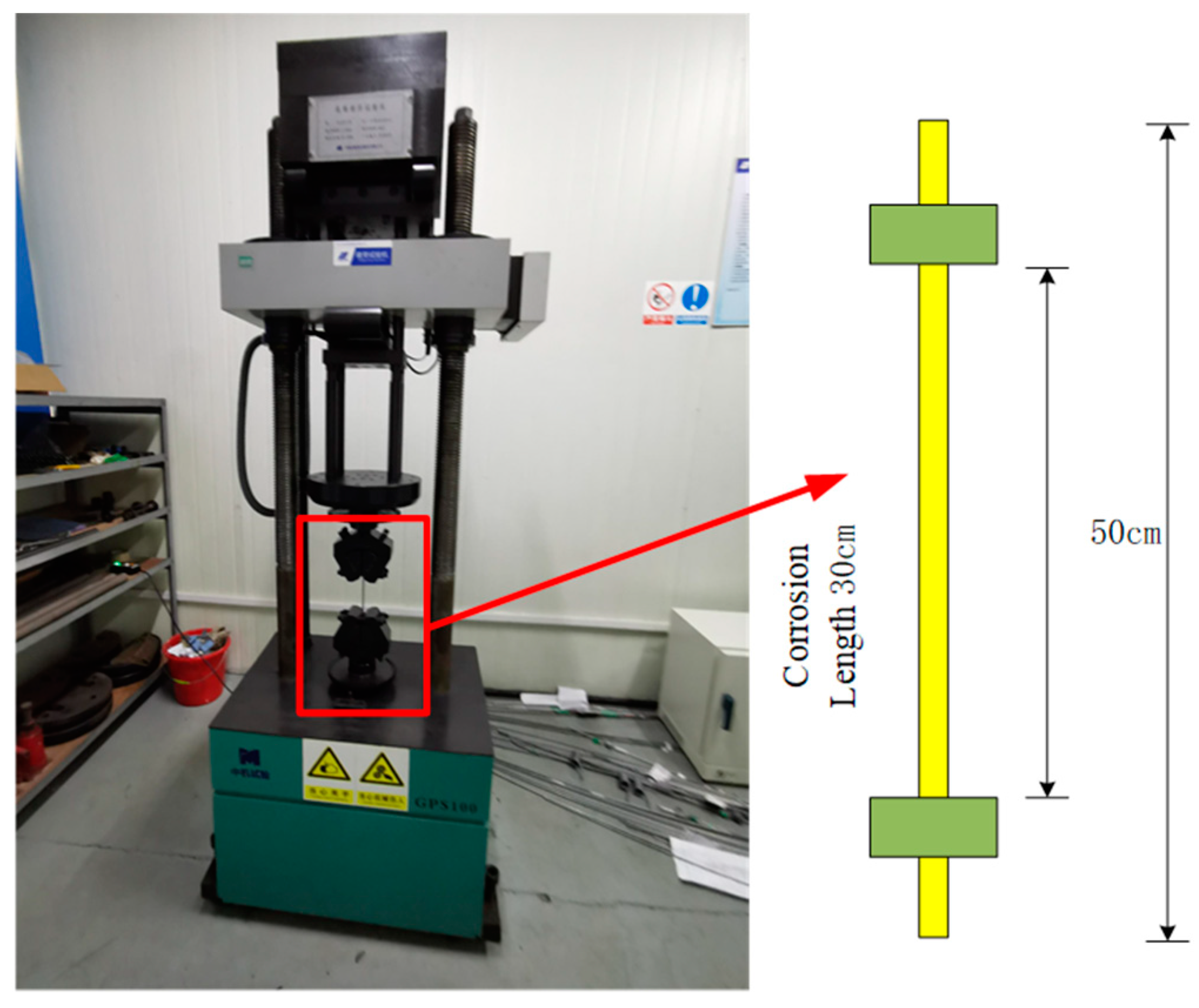
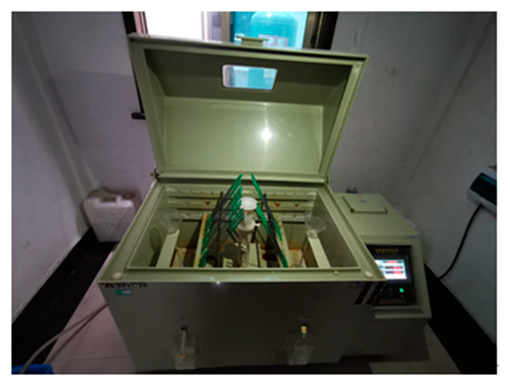
The diameter of the test steel wire is 5 mm and the length of the test specimens is 500 mm, as shown in Figure 1. Both ends are anchored with clamps respectively, and the length of the corroded area is 300 mm. The test specimens used are consistent with the steel wires in the actual bridge slings. Before the corrosion fatigue test, the performance of steel wire must be tested to obtain material parameters, which provide a basis for theoretical analysis in the following text. It tests with a universal testing machine. The test results are shown in

Table 1. Mechanical properties of high strength steel wire specimens.

Sample Number	$\mathbf{E}\left(\mathbf{GPa}\right)$	${\mathsf{\sigma }}_{\mathit{y}}\left(\mathbf{MPa}\right)$	${\mathsf{\sigma }}_{\mathit{u}}\left(\mathbf{MPa}\right)$	$\mathsf{\delta }\left(\mathbf{\%}\right)$
1	201.3	1675	1843	5.7
2	200.8	1656	1851	5.5
3	198.9	1657	1846	5.8
4	199.5	1668	1845	5.6
5	202.4	1671	1863	5.4
Mean	200.58	1665.4	1849.6	5.6

$\mathrm{E}$: elastic modulus; ${\mathsf{\sigma }}_y$: yield strength; ${\mathsf{\sigma }}_u$: ultimate strength; $\mathsf{\delta }$: elongation after fracture.

. From Table 1, it can be seen that the yield stress and limit stress of high-strength steel wire are close, and the plastic stage is not obvious. The brittle fracture of steel wire is more obvious because of the corrosion in an actual working environment. Therefore, corrosion fatigue test is necessary. Corrosion is carried out in a salt mist corrosion tank as showed in Figure 2.

2.2. Corrosion Test

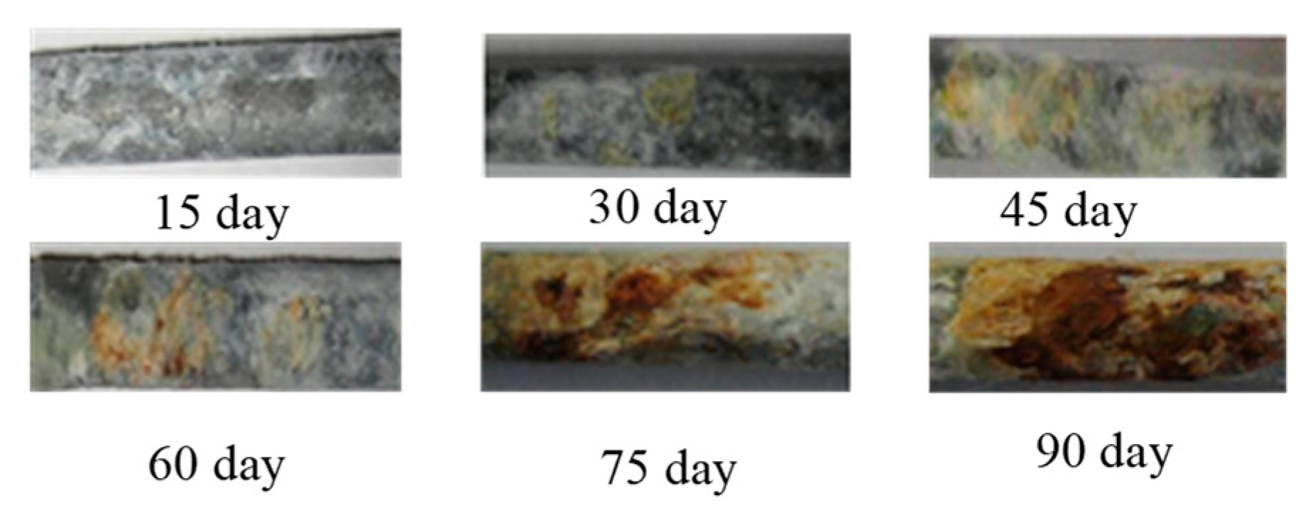
Corrosion of steel wire in an actual bridge may occur only after several years of service. To speed up the experiment, accelerated corrosion experiments are used in this paper, based on the National Standard of the People’s Republic of China [22]. GBT 10125-2012 Corrosion tests in artificial atmospheres salt spray tests, corresponding modifications are made according to the actual conditions of this study to provide preparation for subsequent fatigue tests. The solution consists of 50 g/L of NaCl and HCl with a pH value of 2.9 and was injected into a salt spray test chamber with an over-compressed liquid to simulate the atmosphere. The humidity of the salt spray test chamber was 98% and the temperature was 55 ± 5 °C. The specimens were rotated at intervals to obtain a more uniform degree of corrosion. The samples were placed in a salt spray corrosion tank for different periods to simulate different corrosion levels. The storage time is 15 days, 30 days, 45 days, 60 days, 75 days, and 90 days respectively. Figure 3 shows the corrosion of the specimens at different corrosion time.

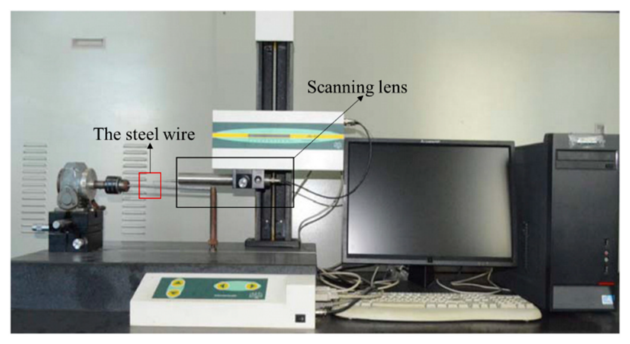
To obtain the surface morphology of corrosion specimens, the non-contact 3D scanner (Fasten, Wuxi, China) was used to scan the corrosion specimens. In the past few years, some scholars have used this equipment to study the shape of the steel plate and steel bar. The equipment used in this paper is shown in Figure 4.

The number and average radius of corrosion pits were measured using the equipment in Figure 4. The measurement results provided a basis for Abaqus to establish a random corrosion pit model. The measurement results are shown in

Table 2. Number and radius of steel wire corrosion pits with different degrees of corrosion.

Sample Number	Number of Corrosion Pits	Average Radius of Corrosion Pit (mm)
1-1	117	0.07
1-2	115	0.09
1-3	119	0.08
1-4	111	0.08
1-5	114	0.07
2-1	212	0.13
2-2	214	0.15
2-3	209	0.16
2-4	205	0.14
2-5	217	0.13
3-1	227	0.19
3-2	238	0.33
3-3	269	0.34
3-4	289	0.36
3-5	245	0.34
4-1	316	0.47
4-2	318	0.49
4-3	319	0.48
4-4	319	0.35
4-5	318	0.49
5-1	398	0.56
5-2	379	0.52
5-3	356	0.54
5-4	378	0.57
5-5	389	0.56
6-1	435	0.76
6-2	456	0.72
6-3	423	0.74
6-4	425	0.72
6-5	418	0.76

.

After the experiment, the specimens were placed indoors to remove the surface corrosion and provide a basis for subsequent work. Corrosion of steel wire can be expressed by loss of quality. The corrosion degree of steel wire is defined as φ. The calculation expression is shown in Equation (1).

$$\mathsf{\phi }=\frac{\mathsf{\Delta }m}{m}=\frac{m_1-m_2-\frac{1}{5}{{\displaystyle \sum }}_{i=1}^5\left[m_{c1}\left(i\right)-m_{c2}\left(i\right)\right]}{m_1\times \frac{l_1}{l_2}}$$

(1)

where $m_1$: quality of corroded specimens;$m_2$: quality of specimens after removing rust by chemical method; $l_1$: length of corrosion zone of specimen; $l_2$: length of the specimen. In practice, chemical methods were used to remove rust while other components of the specimen were unavoidably removed. In order to consider the influence of this factor on the evaluation of corrosion degree, five groups of non-corroded specimens were selected. The quality $m_{c1}\left(i\right)$ of the specimen before treatment by a chemical method and the quality $m_{c2}\left(i\right)$ of the specimen after treatment by a chemical method were measured.

2.3. Fatigue Test

The specimens are tested in the laboratory using a fatigue tester as shown in Figure 1. The loading frequency used in this test is 2 Hz. The stress of the steel wire can be calculated by the Equation (2).

$$\sigma =\frac{F}{A_0}=\frac{F}{\left(\pi /4\right)D_0{}^2}$$

(2)

Among them, F is the axial load of steel wire, and $A_0$ is the cross-section area of non-corroded steel wire. The cross-sectional area can be calculated by diameter. R is defined as stress ratio and S is defined as stress amplitude. They are represented by the following expressions.

$$R={\sigma }_{min}/{\sigma }_{max}$$

(3)

$$S={\sigma }_{max}-{\sigma }_{min}=\left(1-R\right){\sigma }_{max}$$

(4)

where, R = 0.4, S = 270–520 MPa. Fatigue analysis is the focus of this paper. The fatigue test results at different corrosion levels are shown in

Table 3. Corrosion fatigue test results.

Corrosion Time (days)	Sample Number	φ (%)	Lfrac (cm)	S (MPa)	Experimental Number of Cycles
15	1-1	4.72	21.2	520	164,567
	1-2	4.83	22.4	450	224,653
	1-3	4.76	13.4	400	478,456
	1-4	4.52	20.2	360	2,456,345
	1-5	4.96	12.4	270	2467876
30	2-1	8.23	29.2	520	131,345
	2-2	8.45	28.4	450	179,876
	2-3	7.79	27.6	400	367,987
	2-4	8.32	30.1	360	2,324,567
	2-5	8.34	30.4	270	2,333,459
45	3-1	11.12	30.5	520	74,123
	3-2	11.23	21.2	450	126,387
	3-3	11.38	30.1	400	224,278
	3-4	11.56	25.6	360	287,089
	3-5	12.12	27.2	270	1,092,876
60	4-1	14.37	29.7	520	59,346
	4-2	15.12	31.2	450	102,583
	4-3	15.23	18.2	400	132,967
	4-4	14.98	20.3	360	173,261
	4-5	14.99	22.4	270	598,698
75	5-1	18.12	23.4	520	57,896
	5-2	17.97	22.6	450	87,289
	5-3	17.86	24.5	400	103,471
	5-4	18.56	27.8	360	159,826
	5-5	18.02	27.8	270	509,916
90	6-1	19.34	29.2	520	47,647
	6-2	20.12	24.6	450	68,912
	6-3	20.34	25.3	400	98,759
	6-4	20.36	31.1	360	128,798
	6-5	20.37	19.9	270	308,791

L_frac: distance between fracture position and upper part of steel wire.

. The fracture position of the steel wire is between the upper and lower anchorage ends, ranging from 10 to 40 cm. It shows that the fracture of steel wire occurs in the corroded area and the fatigue test result of steel wire is valid.

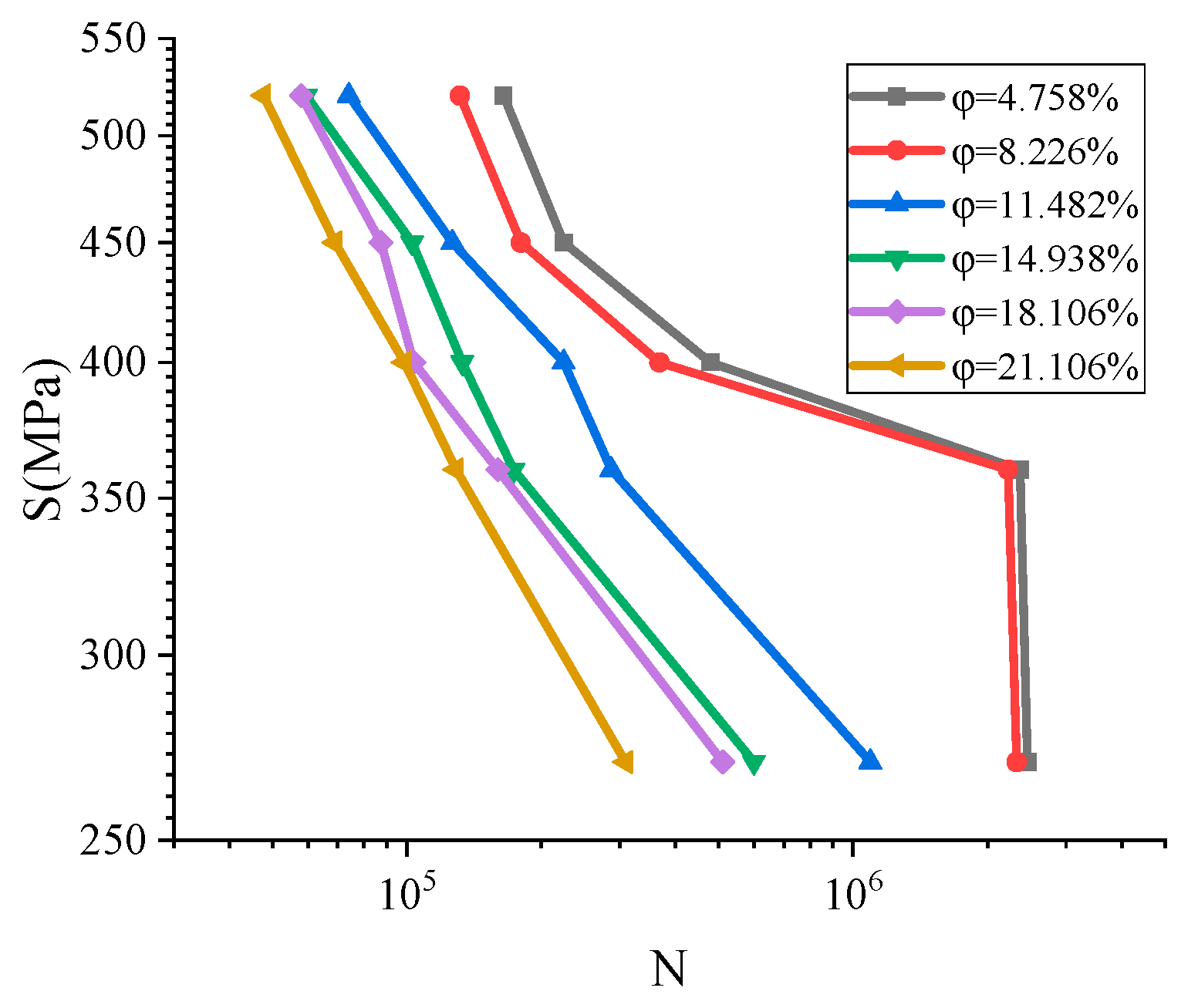
The average corrosion degree of the specimens at different corrosion time in Table 3 is taken as the corrosion degree of the specimens in this group. It can be seen from Figure 5 that the slope of the S-N curve becomes steeper with the increase of corrosion degree and fatigue life decreases faster in the lower-stress range. With the increase of stress amplitude, the fatigue life still decreases rapidly. The life curve becomes very steep, and brittle failure becomes more obvious. In bridge design, the influence of environmental corrosion must be considered in calculating sling fatigue. The effect of corrosion on fatigue is much greater at low stress amplitude than at high-stress amplitude. When the stress amplitude is 520 MPa, the effect of corrosion on fatigue is very small. However, when the stress amplitude is 270 MPa, the effect of corrosion on fatigue is very great. In the low-stress range, corrosion will reduce the nominal fatigue strength, which is equivalent to increasing the fatigue stress. In the high-stress range, fatigue stress is much higher than the nominal fatigue strength, so corrosion has little effect on fatigue in the high-stress range. The corrosion degree increases by only five times and the fatigue life of steel wires decrease to 1/50 of the original one. With the increase of corrosion degree, the S-N curve no longer has an obvious flat part, and the boundary point is about 10%. The typical corrosion fatigue fracture pattern is shown in Figure 6.

As shown in Figure 6, corrosion fatigue fracture of high-strength steel wire can be divided into crack initiation zone, crack propagation zone, and crack fracture zone. Crack initiation zone is formed by processing defects and corrosion during material processing, with an uneven surface. Crack growth zone is caused by the interaction of corrosion and fatigue of high-strength steel wire, which results in crack growth with a smooth and flat surface. The fracture zone can be divided into two parts: the first one is the ductile fracture zone. The second is the brittle fracture zone. As the degree of corrosion increases. The ductile fracture zone gradually becomes brittle fracture zone and the risk of steel wire increases.

3. Numerical Analysis

Corrosion-fatigue is a process of damage and accumulation in materials. Therefore, the evolution equation of corrosion-fatigue damage is as follows:

$$\frac{d{D}_c}{dt}=\frac{c_0+c_1{\left({\sigma }_0+{\sigma }_a\right)}^{\alpha }}{{\left(1-D\right)}^m}$$

(5)

D is the sum of all the damage; D_c is the structural damage caused by corrosion; D_scc is the stress corrosion damage caused by average stress; D_s is the fatigue damage caused by stress amplitude; t is the time; N is the number of cycles (N = ft); T₀ is the period of fatigue load and f is the loading frequency. The relevant expressions are as follows:

$$\frac{d{D}_{scc}}{dt}=c_{scc}{\left(\frac{{\sigma }_0}{1-D}\right)}^{\beta }K$$

(6)

c₀ is the damage accumulation factor under no stress condition. m is the damage coefficient caused by the corrosion. σ₀ and σ_a are the average stress and stress amplitude respectively. c₁(σ₀ + σ_a)^α is the accelerated effect of stress on corrosion damage. α is a constant related to materials.

$$\frac{d{D}_{scc}}{dt}=c_{scc}{\left(\frac{{\sigma }_0}{1-D}\right)}^{\beta }K$$

(7)

$$K=\{\begin{array}{c}1-{\left(\frac{\left(1-D\right){\sigma }_{scc}}{{\sigma }_0}\right)}^{\gamma } , \frac{{\sigma }_0}{1-D}>{\sigma }_{scc}\\ 0 , others \end{array}$$

(8)

$c_{scc}$ is the cumulative coefficient of stress corrosion damage, ${\sigma }_{scc}$ is the threshold value of stress corrosion, and γ is a constant related to the material.

$$\frac{d{D}_s}{dN}={\left(1-D\right)}^{-u}{\left(\frac{{\sigma }_a}{M\left({\sigma }_0\right)}\right)}^{\omega }$$

(9)

$u,\omega$ is experimental constant,$M\left({\sigma }_0\right)$ is the material parameter related to the average stress.

$$\frac{dD}{dt}=\frac{c_0+c_1{\left({\sigma }_0+{\sigma }_a\right)}^{\alpha }}{{\left(1-D\right)}^m}+c_{scc}{\left(\frac{{\sigma }_0}{1-D}\right)}^{\beta }K+{\left(1-D\right)}^{-u}f{\left(\frac{{\sigma }_a}{M\left({\sigma }_0\right)}\right)}^{\omega }$$

(10)

The fatigue life of steel wire can be calculated by embedding the constitutive Equation (12) into Abaqus. The parameters in the equation can be fitted by experiments.

$$\mathsf{\sigma }=\left(1-D\right)E\epsilon$$

(11)

Abaqus was used to calculate the specimens in Table 3, and the calculation results are shown in

Table 4. Comparison results of fatigue life.

Corrosion Time (days)	Sample Number	Calculated Number of Cycles	Error (%)
15	1-1	134,789	18.09
	1-2	193,498	13.87
	1-3	398,732	16.66
	1-4	2,154,346	12.29
	1-5	2,163,837	12.32
30	2-1	117,964	10.19
	2-2	169,987	5.50
	2-3	328,976	10.60
	2-4	2,129,876	8.38
	2-5	2,132,435	8.61
45	3-1	61,987	16.37
	3-2	105,132	16.82
	3-3	201,765	10.04
	3-4	265,410	7.55
	3-5	1,051,123	3.82
60	4-1	51,987	12.40
	4-2	103,263	0.66
	4-3	109,876	17.37
	4-4	148,654	14.20
	4-5	512,189	14.45
75	5-1	52,678	9.01
	5-2	79,777	8.61
	5-3	92,345	10.75
	5-4	134,234	16.01
	5-5	480,001	5.87
90	6-1	39,213	17.70
	6-2	60,021	12.90
	6-3	87,879	11.02
	6-4	107,123	16.83
	6-5	291,176	5.70

and Figure 7.

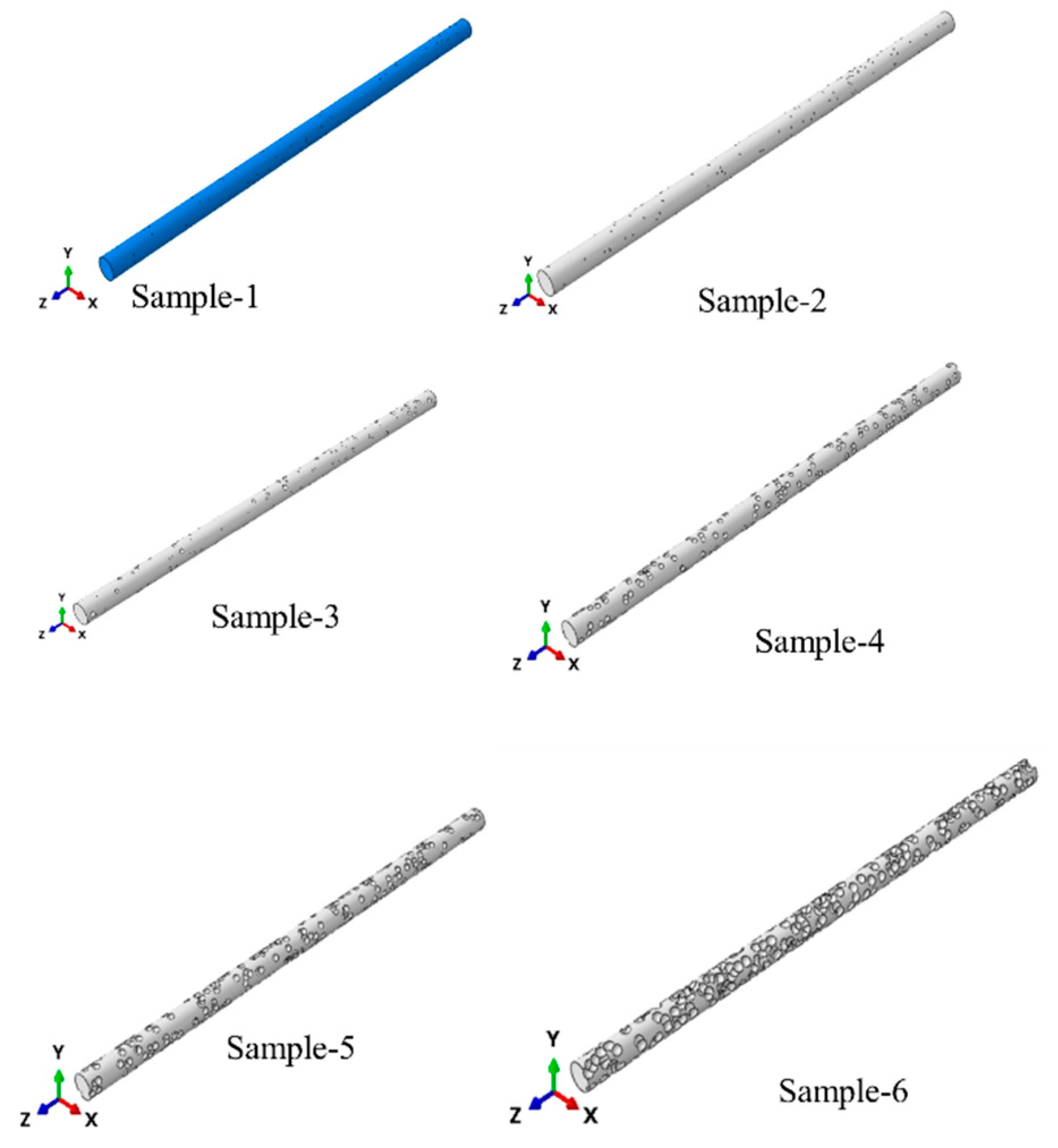
The geometrical dimension of the finite element model is the same as that of the test specimens. As showing in Figure 8, taking the average value of the number and radius of corrosion pits of each group of test pieces in Table 2 as parameters, a random corrosion model was established in Abaqus through Python. Under the same load, the stress change of the wire of different element sizes is within 5%, and the element size is considered to be the appropriate size at this time.

The corrosion region is the tetrahedral element (C3D10) with a size of 0.2 mm. Corrosion pits were randomly produced in the corrosion area of the finite element model by Python in Abaqus. The mass lost by the finite element model of steel wire with corrosion pit is equal to that lost by the corrosion test. The initial tension and fatigue load were applied to the finite element model by using the cooling method shown in Equations (12) and (13).

$$\mathsf{\Delta }\mathrm{T}=\frac{\sigma }{\alpha E}$$

(12)

$$\mathsf{\Delta }\mathsf{\Delta }\mathrm{T}=\frac{\mathsf{\Delta }\sigma }{\alpha E}=\frac{S}{\alpha E}$$

(13)

The reference temperature is 0 °C in this paper. Where,$\mathsf{\Delta }\mathrm{T}$: change in temperature;$\sigma$: stress of steel wire;$\alpha$: coefficient of thermal expansion of steel wire;$\mathsf{\Delta }\mathsf{\Delta }\mathrm{T}$: secondary change of temperature; $\alpha =1.2\times {10}^{-5}$; $E=2.1\times {10}^5 \mathrm{MPa};\sigma =500 \mathrm{Mpa}$. According to Equation (12), the initial temperature of the finite element model is −198 °C. Thus, the initial tension of the steel wire is realized. Second, the change of the temperature can be obtained by taking S in the Table 3 into Equation (13). The cyclic change of temperature can be realized by using the function of direct cyclic load in Abaqus, and finally the fatigue load of the finite element model can be achieved.

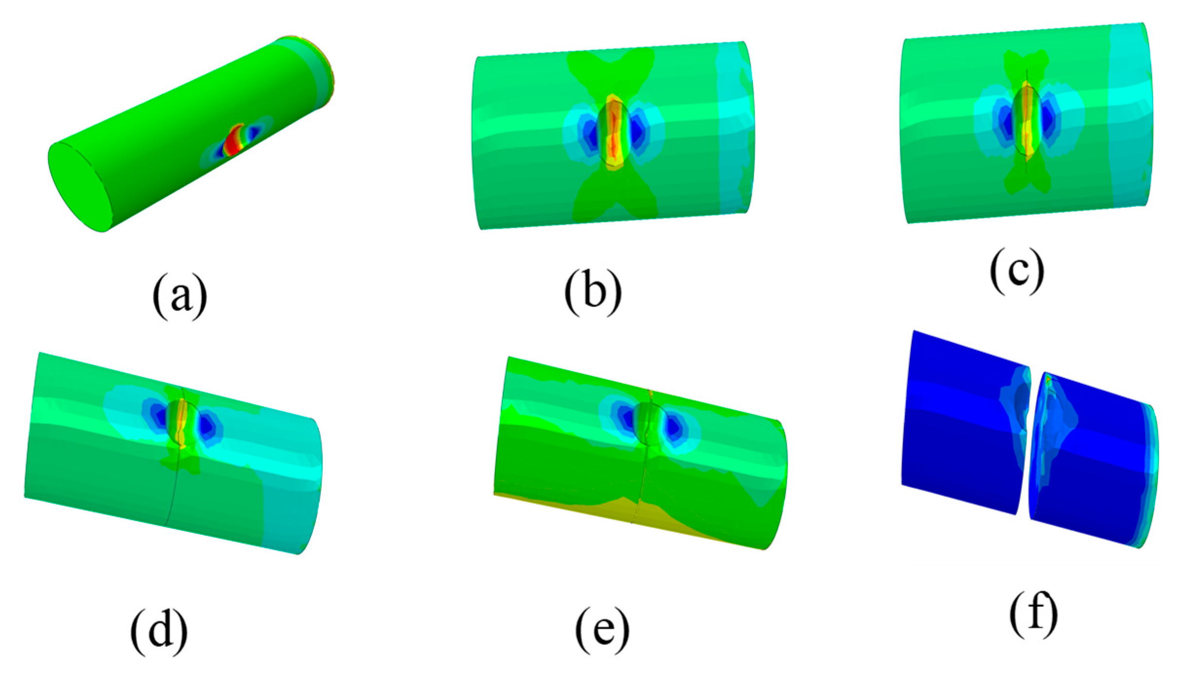
The constitutive model of high-strength steel wire can be considered as the bilinear hardening model. In this paper, the extended finite element method is used to simulate the fatigue fracture of steel wire.${\sigma }_y=1675 \mathrm{MPa},{\sigma }_u=1860 \mathrm{MPa}$ are selected in the finite element model. The failure criterion is chosen as the maximum principal stress criterion in Abaqus. According to Equation (11), the stress of steel wire increases gradually. When it exceeds the limit stress, the element breaks. Thus, crack growth can be realized. The typical fracture process near the corrosion pit is shown in Figure 9.

It can be seen from Figure 9 that under the condition of corrosion, stress concentration is generated near the corrosion pit, where the fatigue crack is initiated. The fracture process of high strength steel wire under corrosion fatigue interaction was simulated in Figure 9. Figure 9a shows stress concentration near the corrosion pit of high strength steel wire and Figure 9b shows the crack initiation near the corrosion pit. Figure 9c shows the crack growth near the corrosion pit. Figure 9d,e show further crack growth. Figure 9f shows the corrosion fatigue fracture of high strength steel wire.

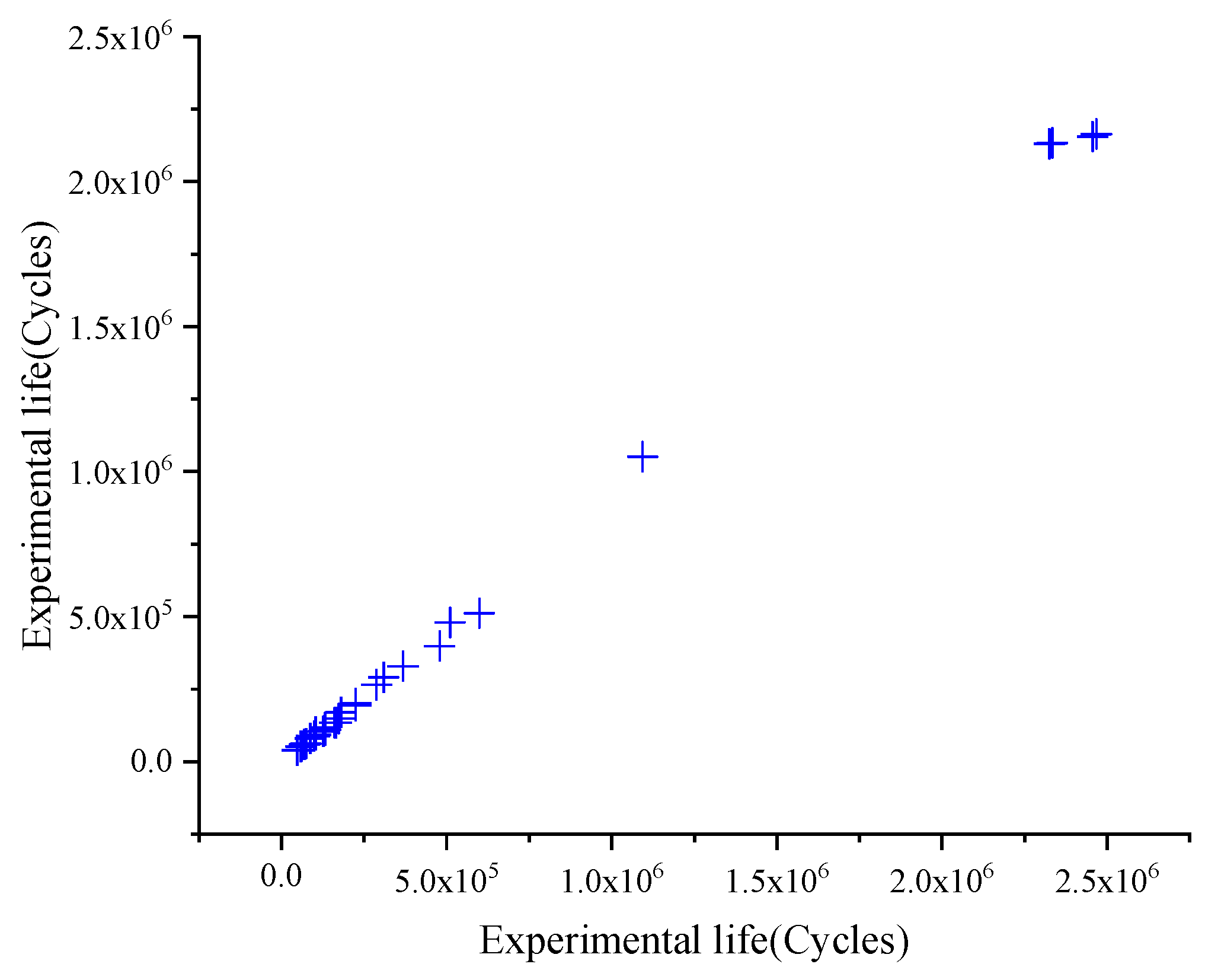
Table 4 shows that the maximum error of fatigue life predicted by the theoretical model is close to 20%, and the average error is more than 10%. The fatigue life predicted by the theoretical model is lower than that of the test results. The phenomenon is mainly caused by the following reasons:

(1). The prediction model is different from the actual situation.

(2). The coupling effect of corrosion and fatigue was considered in the prediction model, but the effect was not considered in the experiment in this paper.

Although the error between the prediction model and the test is large, the calculation results are conservative and can be considered reliable. In practice, the results of the corrosion-fatigue are quite discrete. The prediction model is simple and practical.

4. Conclusions

Considering the coupling effect of corrosion and fatigue on the sling in practical engineering, the basic high strength steel wires were selected as the test specimens. The fatigue tests were carried out on the specimens after different degrees of corrosion. The S-N curves of different degrees of corrosion were given and the steel wire life model considering the effect of corrosion was proposed. There are several conclusions and prospects as follows.

(1). The effect of the corrosion on the fatigue of high strength steel wire cannot be neglected. The larger the corrosion degree, the steeper the S-N curve, and a sudden change may occur when the stress amplitude is large.

(2). The influence of corrosion was considered in the prediction model proposed in this paper. In this paper, a random corrosion pit model was established. In a corrosive environment, corrosion pits are formed on the surface of the steel wire, and stress concentration appears at the bottom of the corrosion pits. With the loading of the fatigue load, the corrosion pit becomes a crack and develops until it breaks. Corrosion fatigue failure of steel wire can be divided into the following stages: pitting growth, expansion to the stage of small cracks, the stage of transition of toughness and brittleness after cracks appear, and the stage of breaking.

(3). This article studies the fatigue test under different corrosion conditions. How to design the test considering the corrosion fatigue coupling effect at the same time needs to be further studied.

References

- Xue, S.; Shen, R. Real time cable force identification by short time sparse time domain algorithm with half wave. Measurement 2020, 152, 107355. [Google Scholar] [CrossRef]
- Zhou, Y.; Chen, S. Investigation of the live-load effects on long-span bridges under traffic flows. J. Bridge Eng. 2018, 23, 04018021. [Google Scholar] [CrossRef]
- Guo, T.; Liu, Z.; Correia, J.; de Jesus, A.M. Experimental study on fretting-fatigue of bridge cable wires. Int. J. Fatigue 2020, 131, 105321. [Google Scholar] [CrossRef]
- Lesiuk, G.; Rymsza, B.; Rabiega, J.; Correia, J.A.; De Jesus, A.; Calcada, R. Influence of loading direction on the static and fatigue fracture properties of the long term operated metallic materials. Eng. Fail. Anal. 2019, 96, 409–425. [Google Scholar] [CrossRef]
- Chang, X.-D.; Peng, Y.-X.; Zhu, Z.-C.; Zou, S.-Y.; Gong, X.-S.; Xu, C.-M. Evolution Properties of Tribological Parameters for Steel Wire Rope under Sliding Contact Conditions. Metals 2018, 8, 743. [Google Scholar] [CrossRef] [Green Version]
- Xue, S.; Shen, R.; Chen, W.; Miao, R. Corrosion fatigue failure analysis and service life prediction of high strength steel wire. Eng. Fail. Anal. 2020, 110, 104440. [Google Scholar] [CrossRef]
- Wang, Y.; Zheng, Y.; Zhang, W.; Lu, Q. Analysis on Damage Evolution and Corrosion Fatigue Performance of High-strength Steel Wire for Bridge Cable: Experiments and Numerical Simulation. Theor. Appl. Fract. Mech. 2020, 102571. [Google Scholar] [CrossRef]
- Xue, S.; Shen, R.; Shao, M.; Chen, W.; Miao, R. Fatigue failure analysis of steel wire rope sling based on share-splitting slip theory. Eng. Fail. Anal. 2019, 105, 1189–1200. [Google Scholar] [CrossRef]
- Ni, Y.Q.; Ye, X.W.; Ko, J.M. Monitoring-Based Fatigue Reliability Assessment of Steel Bridges: Analytical Model and Application. J. Struct. Eng. 2010, 136, 1563–1573. [Google Scholar] [CrossRef]
- Zhao, Z.W.; Haldar, A.; Breen, F.L. Fatigue-Reliability Evaluation of Steel Bridges. J. Struct. Eng. 1994, 120, 1608–1623. [Google Scholar] [CrossRef]
- Adasooriya, N.D.; Siriwardane, S.C. Remaining fatigue life estimation of corroded bridge members. Fatigue Fract. Eng. Mater. Struct. 2014, 37, 603–622. [Google Scholar] [CrossRef]
- Zampieri, P.; Curtarello, A.; Maiorana, E.; Pellegrino, C. A Review of the Fatigue Strength of Shear Bolted Connections. Int. J. Steel Struct. 2019, 19, 1084–1098. [Google Scholar] [CrossRef]
- Zampieri, P.; Curtarello, A.; Pellegrino, C.; Maiorana, E. Fatigue strength of corroded bolted connection. Frat. Integrità Strutt. 2018, 12, 90–96. [Google Scholar] [CrossRef] [Green Version]
- Zampieri, P.; Curtarello, A.; Maiorana, E.; Pellegrino, C. Numerical analyses of corroded bolted connections. Procedia Struct. Integr. 2017, 5, 592–599. [Google Scholar] [CrossRef]
- Zampieri, P.; Curtarello, A.; Maiorana, E.; Pellegrino, C.; De Rossi, N.; Savio, G.; Concheri, G. Influence of corrosion morphology on the Fatigue strength of Bolted joints. Procedia Struct. Integr. 2017, 5, 409–415. [Google Scholar] [CrossRef]
- Toribio, J.; Ovejero, E. Effect of cold drawing on microstructure and corrosion performance of high-strength steel. Mech. Time-Depend. Mater. 1997, 1, 307–319. [Google Scholar] [CrossRef]
- Aleksandrov Fabijanić, T.; Kurtela, M.; Škrinjarić, I.; Pötschke, J.; Mayer, M. Electrochemical Corrosion Resistance of Ni and Co Bonded Near-Nano and Nanostructured Cemented Carbides. Metals 2020, 10, 224. [Google Scholar] [CrossRef] [Green Version]
- Zhang, W.-P.; Li, C.-K.; Gu, X.-L.; Zeng, Y.-H. Variability in cross-sectional areas and tensile properties of corroded prestressing wires. Constr. Build. Mater. 2019, 228, 116830. [Google Scholar] [CrossRef]
- Marandi, L.; Sen, I. Effect of Saline Atmosphere on the Mechanical Properties of Commercial Steel Wire. Metall. Mater. Trans. A 2019, 50, 132–141. [Google Scholar] [CrossRef]
- Li, L.; Mahmoodian, M.; Li, C.-Q.; Robert, D. Effect of corrosion and hydrogen embrittlement on microstructure and mechanical properties of mild steel. Constr. Build. Mater. 2018, 170, 78–90. [Google Scholar] [CrossRef]
- Fang, K.; Li, S.; Chen, Z.; Li, H. Geometric characteristics of corrosion pits on high-strength steel wires in bridge cables under applied stress. Struct. Infrastruct. Eng. 2020, 1–15. [Google Scholar] [CrossRef]
- National Standard of the People’s Republic of China. GBT 10125-2012 Corrosion Tests in Artificial Atmospheres-Salt Spray Tests; Standards Press of China: Beijing, China, 2012. [Google Scholar]
Figure 1.
Area diagram of corroded steel wire.
Figure 2.
Salt spray corrosion tank used for corrosion.
Figure 3.
Corrosion of test piece.
Figure 4.
Non-contact 3D scanner.
Figure 5.
The S-N curves under different corrosion degrees.
Figure 6.
Corrosion fatigue fracture morphology. (a) Corrosion pit evolution diagram; (b) Steel wire fracture diagram near corrosion pit.
Figure 7.
Correlation between experimental life and predicted life.
Figure 8.
Finite model in Abaqus.
Figure 9.
Crack growth process in Abaqus. (a) The stress concentration near the corrosion pit; (b) the crack initiation near the corrosion pit; (c) The crack growth near the corrosion pit (d) Crack growth-I; (e) Crack growth-II; (f) The corrosion fatigue fracture of high strength steel wire.