Flow Stress of Ti-6Al-4V during Hot Deformation: Decision Tree Modeling

1
Metal Forming R&D Group, Korea Institute of Industrial Technology, 156 Gaetbeol-ro, Yeonsu-gu, Incheon 21999, Korea
2
Department of Smart Automobile, Soonchunhyang University, 22 Soonchunhyang-ro, Sinchang-myeon, Asan-si, Chungcheongnam-do 31538, Korea
*
Author to whom correspondence should be addressed.
Metals 2020, 10(6), 739; https://doi.org/10.3390/met10060739
Submission received: 10 April 2020
/
Revised: 26 May 2020
/
Accepted: 27 May 2020
/
Published: 2 June 2020
Abstract
:In this study, the flow stress of Ti-6Al-4V during hot deformation was modeled using a decision tree algorithm. Hot compression experiments for Ti-6Al-4V in a Gleeble-3500 thermomechanical simulator were performed under a strain rate of 0.002–20 s–1 and temperatures of 575–725 °C. After the experiments, flow stress behavior was modeled, first by a traditional Arrhenius type equation, second by utilizing the artificial neural network, and lastly, with the aid of the decision tree algorithm. While the characteristics of measured flow stress were noticeably dependent on the resulting strain rate and temperature, the modeling accuracy regarding the flow stress results of the Arrhenius type equation, neural network approach and decision tree algorithm were compared. The decision tree algorithm predicted the flow stress most effectively.
1. Introduction
Ti-6Al-4V is a titanium alloy consisting of Al (6 wt%) and v (4 wt%). The alloy is known for its good mechanical properties, toughness, high strength, low density and corrosion resistance [1,2,3]. Since it has superior properties, the alloy is used in a variety of areas such as pressure vessels, automobile parts, aerospace, as well as used for the manufacturing of medical parts [2,4,5,6].
For instance, in aerospace, Ti-6Al-4V is used for airframes as seat rails, general structural material, bolts and engine parts such as fan blades and fan casing [4]. Additionally, the alloy is used to manufacture intake valves in the automobile industry [5]. In the medical field, the alloy is used for surgical implants, due to its ability to perform satisfactorily in the temperature range of 23 °C to 150 °C [6].
Despite the final product’s excellent mechanical properties and the alloy’s popularity in a variety of fields, metal processing of Ti-6Al-4V is not convenient due to its high strength. Therefore, metal processing of Ti-6Al-4V is usually performed in a high temperature environment, which increases the ductility of the alloy. The ordinary temperature of hot forming of Ti-6Al-4V is 730 °C [7], and the examples of hot forming methods for Ti-6Al-4V include superplastic forming, hot brake forming, hot power spinning and hot stamping [7,8]. Superplastic forming is the commonly used method due to good formability of complex parts, the part’s quality with lighter weight and efficient structures, and the ability to put equal pressure on all areas of the material being formed while working on it [7,8]. The temperature range of superplastic forming of Ti-6Al-4V is 870–925 °C [7].
However, the existing methods of Ti-6Al-4V forming have low efficiency due to low strain rate in the forming process, and are relatively expensive due to heating of the workpiece and tool [8]. In this regard, the method of hot stamping is arising as a preferred method to use this material [8,9]. Kopec et al. [8] carried out novel hot stamping of Ti-6Al-4V with low temperature tools and studied the feasibility of the process. In the utilization of this method, the titanium alloy parts could be produced well in the temperature range of 750–850 °C. Hamedon et al. [9] performed hot stamping of Ti-6Al-4V along with resistance heating. From the two references, the hot stamping method could achieve a level of improved productivity by heating the titanium sheet with resistance heating, eliminating the die heating process and reducing the heating time. In addition, the resistance heating used in the bending process could reduce oxidation and springback of the titanium workpiece.
For hot working of the Ti-6Al-4V alloy, it is essential to develop constitutive equations of the titanium alloy for the hot deformation. So far, performed various experiments have employed various types of constitutive equations for various ranges of strain rates and temperatures. Cai et al. [3] performed hot compression tests for Ti–6Al–4V alloys at temperatures of 800–1050 °C and a strain rate of 0.0005–1 s−1 to model the flow stress using an Arrhenius equation. Porntadawit et al. [10] also performed hot compression tests for Ti–6Al–4V at 900–1050 °C and 0.1–10 s−1 strain rate. In these two studies, the flow stress was modeled using the Shafiei and Ebrahimi constitutive equation, Cingara constitutive equation and an Arrhenius type equation. Nguyen et al. [2] performed tensile experiments for Ti-6Al-4V at a temperature range of 400–700 °C and modeled the flow stress using a modified form of the Fields–Backofen equation. Additionally, Zhang et al. [11] carried out a hot tensile test at a temperature range of 650–750 °C and 0.0005–0.05 s−1 strain rate. The Arrhenius equation and a modified type of Norton–Hoff equation were used for the determination of a constitutive model. The research found that while both constitutive models could predict most of the flow stress, the use of a modified type of Norton–Hoff equation is more accurate than the Arrhenius model. Furthermore, Brusch et al. [12] carried out a hot compression test at a temperature range of 880–950 °C and a strain rate of 1–50 s−1 to study the hot workability of the Ti-6Al-4V alloy. In the research, the flow stress was modeled using Zener–Hollomon parameters. However, traditional constitutive models often show limited accuracy in the prediction of flow stress during hot deformation. Some of the reasons are due to the inherent limitation in predicting the non-linear relation of process parameters and flow stress, and the fact that a regression approach of the constitutive equation cannot capture all data including the dispersed data [13,14].
In an effort to develop a more precise prediction model of the hot deformation of metals, a neural network approach was also employed. Wen et al. [1] carried out compression tests for Ti-6Al-4V at the temperature range of 1053–1023 K with a strain rate of 0.01–10 s−1, and developed a neural network model to predict flows stress of the Ti-6Al-4V. The neural network model showed a strong ability to predict the deformation behavior of Ti-6Al-4V. Quan et al. [15] performed a hot compression test for 20MnNiMo alloy at a temperature range of 900–1200 °C and 0.01–10 s−1 strain rate, and developed an improved Arrhenius type and neural network model. The neural network model showed a greater predictability than the improved Arrhenius model. Sun et al. [16] also carried out a compression test for Ti-47Al-2Nb-2Cr at a temperature range of 950–1200 °C and strain rate of 10 s−3–10 s−1 to develop the back-propagation neural network model. On comparison, the neural network model has better accuracy than the traditional Arrhenius type model. Sabokpa et al. [13] carried out hot compression tests for cast AZ81 magnesium alloy at a temperature range of 250–400 °C and strain rates of 0.0001 s−1, 0.001 s−1 and 0.01 s−1, where flow stress was modeled by the Arrhenius type equation and neural network approach. They also reported that the neural network approach was more accurate and efficient than the Arrhenius type equation in modeling the flow stress. The literature survey shows that neural network models produce better predictions than the traditional constitutive equations. However, the neural network approach needs some improvements in modeling efficiency. Developing the model would need some optimization work by choosing appropriate numbers of layers and neurons, parameters and detailed resolution algorithms.
Although various researchers achieved significant improvements, a successful prediction of the stress–strain relation during the hot deformation of metal is yet to be achieved. Therefore, there is an obvious need for developing a prediction model with high accuracy and efficiency. In this research, a decision tree algorithm was employed for the prediction of flow stress. Although the stress–strain response of large strain deformation of alloys can be most robustly obtained by the combined work of tensile and shear deformations [17,18], the presented research considers the aspect of challenges in high temperature tests. Therefore, the compression tests in elevated temperatures were carried out to measure the stress–strain responses of Ti-6Al-4V. In detail, hot compression tests for Ti-6Al-4V were done at a temperature range of 575–725 °C and strain rate of 0.002–20 s−1. In the present research, testing is performed only once per test condition and a more detailed experimental investigation will be performed in future. After the test, the stress–strain relation was modeled by an Arrhenius equation, artificial neural network and a decision tree approach. Performances of the three approaches were studied based on prediction accuracy and efficiency.
2. Materials and Methods
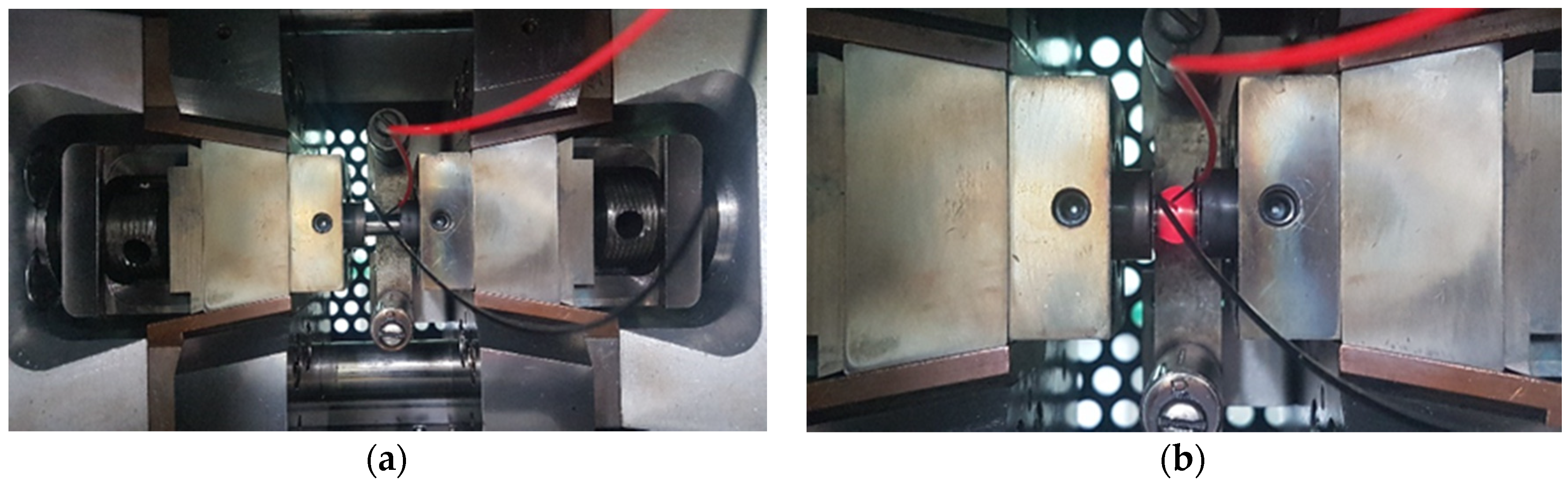
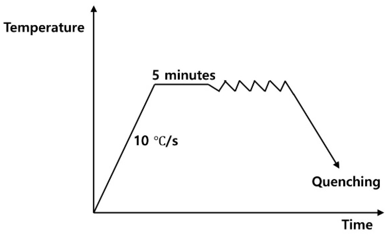
For the hot deformation test, a cylindrical specimen of Ti-6Al-4V was prepared. The specimen’s size was 10 mm in diameter and 15 mm in length. For the test, a Gleeble-3500 system (Dynamic Systems Inc., New York, NY, USA) was used in a thermo-mechanical simulator. The simulator was equipped with a servo hydraulic system, data acquisition system as well as a fast heating system. Figure 1 shows the picture of (a) the mounted specimen in the Gleeble 3500 simulator and (b) the specimen during the hot compression test. To measure the specimen temperature, an R-type thermocouple was spot welded at the middle of the specimen. On the simulator, isothermal hot compression tests were carried out at a temperature range of 750–850 °C with 50 °C intervals and strain rates of 0.002 s−1, 0.02 s−1, 2 s−1 and 20 s−1. During the compression test, the temperature was increased by 10 °C/s to the target (deformation) temperature, after which the specimen was held for five minutes before the compression. After the compression, the specimen was gas-quenched. Figure 2 represents the temperature change of the specimen during the isothermal compression test.
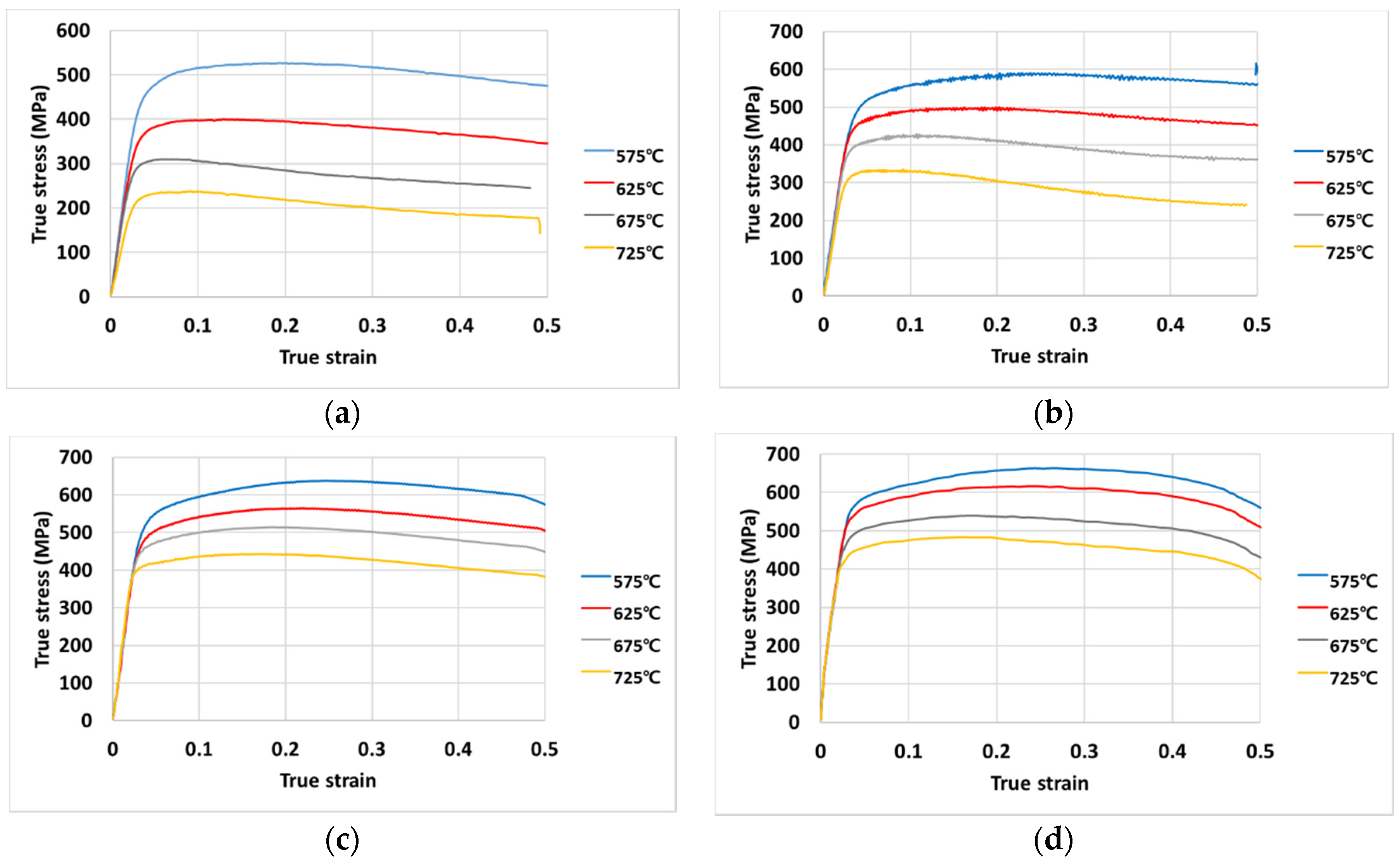
Figure 3 shows the true stress–strain curves when the strain rates were (a) 0.002 s−1, (b) 0.02 s−1, (c) 2 s−1 and (d) 20 s−1, respectively and strain ranged from 0–0.5. The flow stresses for different strain rates and temperatures show that the flow stress behavior of Ti-6Al-4V is highly dependent on the resulting strain rate and temperature. Generally, an increase in temperature leads to a decrease in flow stress, and an increase in strain rate leads to an increase in flow stress. Both softening and hardening of flow stress were observed after yield (for example, at 725 °C under 0.002 s−1). The softening of the flow stress is considered to be caused by recrystallization below the beta transus temperature.
2.1. Arrhenius Equation
The relationship between flow stress, strain rate and temperature can be described by an Arrhenius equation with Zener–Hollomon parameter Z as below:
where
where Q is the activation energy (J/mol), R is gas constant (J/(mol∙K)), T is the absolute temperature (K) and is strain rate. α, β, n’, n, A are material constants where α = β/n’.
The above materials constants for the equations that vary with strain can be determined from the experimental results. Substituting the Equations in (3) to (2) and taking logarithm of both sides of the three resultant equations gives three equations as follows:
where B and C are constants.
In (4), the constant n can be obtained from slope of the plots. The β in (5) can be obtained from slope of the plots.
Thus, α can be obtained from α = β/n’. The constant n in (6) can be calculated from plots. Using Equations (1) and (2), Q and Z can be obtained.
2.2. Neural Network
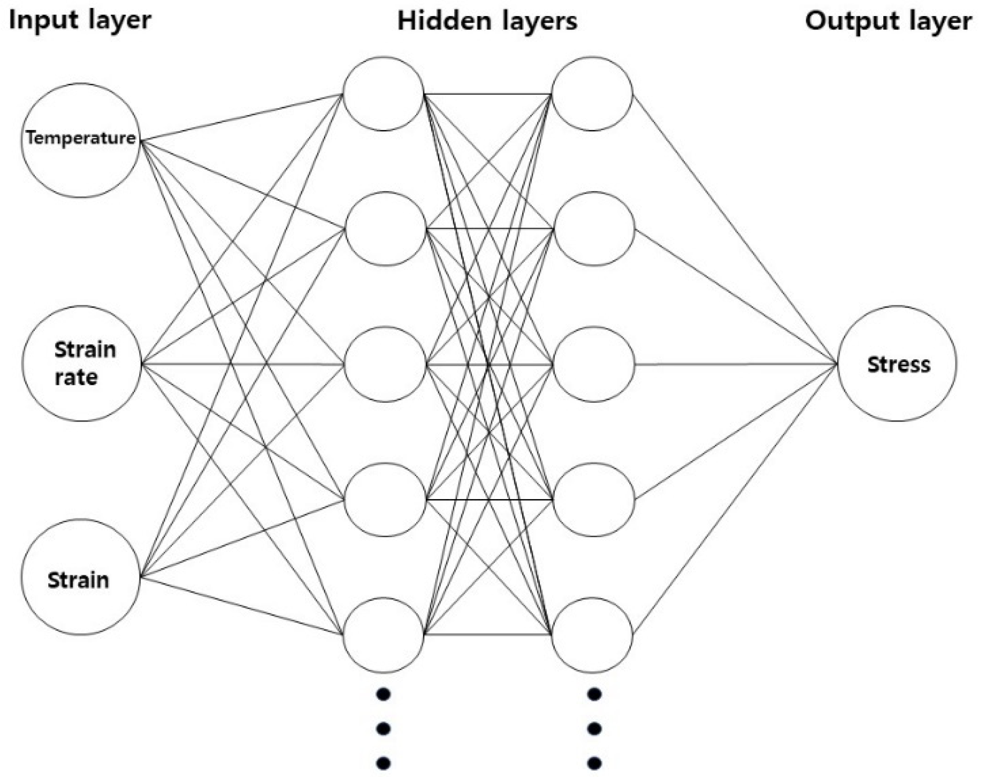
Figure 4 is a diagram representing the structure of the neural network. In this case, the neural network is composed of three types of layers: the input layer, hidden layer, and output layer. Each type of layer consists of a processing unit known as a neuron. The number of hidden layers and neurons have a direct influence on the effectiveness of the neural network operation. Sun et al. [16] used 20 neurons in one hidden layer. Wen et al. [1] and Quan et al. [15] used 14 and 23 neurons in hidden layers respectively. Each neuron in the layers has a weight number, which is multiplied by the numbers received from the neurons found in the previous layer. After using a calculation that gives numbers to the latter layers in order, the number in the output layer becomes the neural network’s output. In this research, the neural network was designed with the input layer containing three neurons representing temperature, strain rate and strain. This research also employed two hidden layers with 85 neurons for each hidden layer. The output layer had one neuron that represents flow stress. In training the neural network, a particular dataset prepared for the training is checked repeatedly and weight values adjusted accordingly.
Successfully developing a neural network model needs the best set of weight values for each neuron. In this model, the most popular training algorithm [13], back-propagation, is used with an ADAM optimization algorithm. In the current model, learning rate was 0.001 and weight decay was 0.1. The python package Keras was used for the development of the model. During training, the performance of the neural network was continuously evaluated by loss function. The loss function used in this model was mean square error as is noted below:
where n is the data index, is output value and is the reference value.
The RELU (Rectified linear unit) function was chosen for portraying the activation function of hidden layer. For training of the neural network model, 576 data points were randomly chosen from a strain range of 0.05–0.45 on the 16 stress–strain curves, and another 144 data points were used to test the trained neural network model. Table 1 shows parameters for the neural network model.
2.3. Decision Tree Modeling
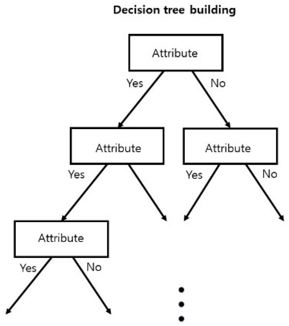
Figure 5 shows the schematic diagram of a decision tree algorithm. Starting from the top node (root node), the decision tree algorithm performs the action of splitting the dataset by checking the classifying attributes. At the sub nodes (child node), the split dataset is further split by other classifying attributes. This consequent splitting builds a tree-like structure, until the dataset is finally split into multiple classes. In other words, the decision tree is a logical combination of sequential tests [19]. If the target class characteristics are numeric, the decision tree algorithm can be used as regression algorithm. To this end, various types of decision tree algorithms were developed (ID3, C4.5, C5.0, SCPRINT, CART, SLIQ) [19], and a classification and regression tree (CART) was used in this study’s regression analysis. The Python package scikit-learn was used to implement the decision tree algorithm. In the current model, mean squared error (MSE) was used for the regression criterion. The tree depth is not fixed in the model. While there are three attributes, namely temperature, strain rate and strain, one attribute is considered at each split. Table 2 shows the parameters used in the decision tree model.
3. Results and Discussion
3.1. Arrhenius Equation
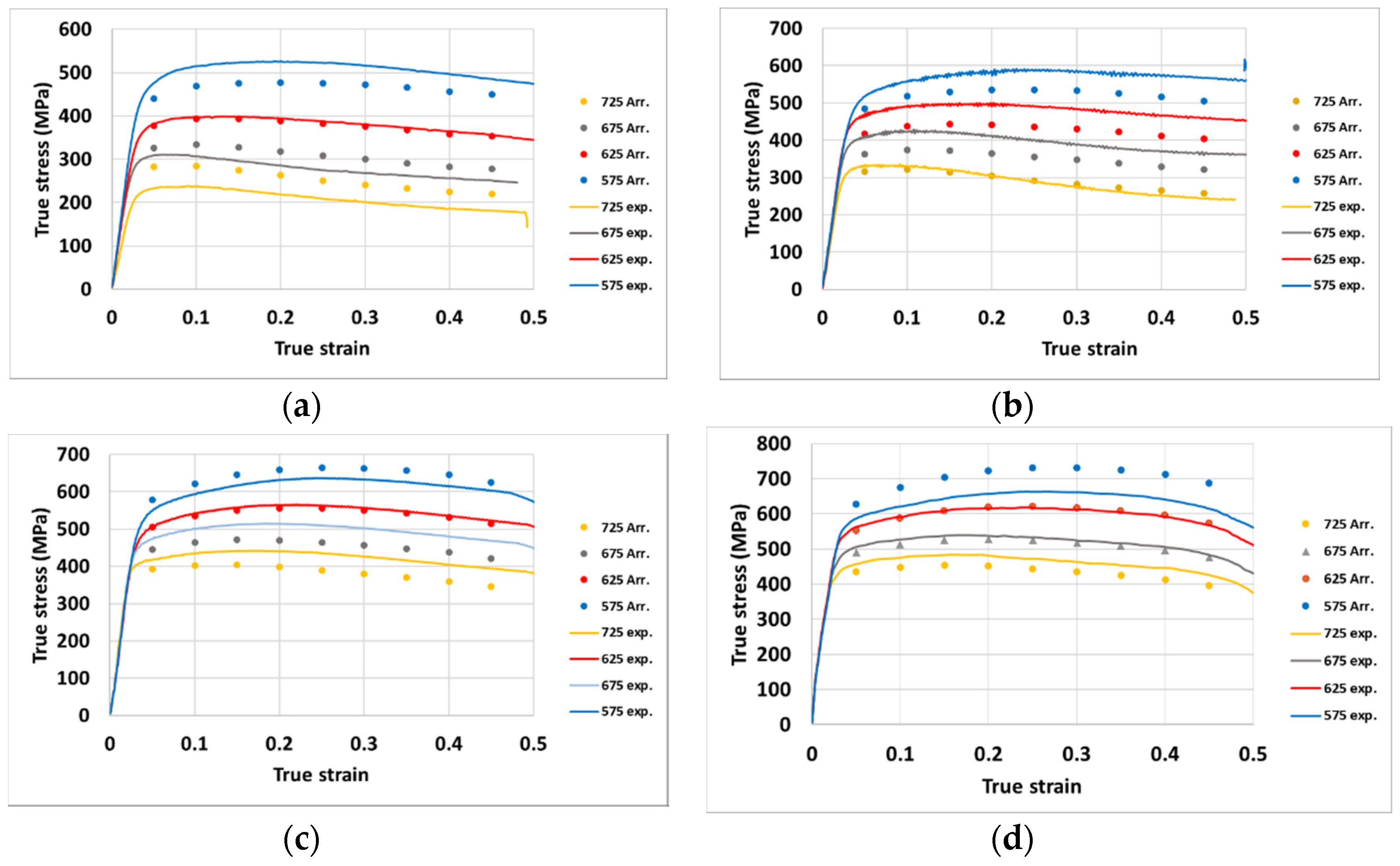
Figure 6 shows the stress–strain plots calculated by an Arrhenius equation at a strain value of 0.05 to 0.45, with intervals of 0.05. The calculated stresses are marked in the figure with the experimental curves at a strain rate of (a) 0.002 s−1, (b) 0.02 s−1, (c) 2 s−1 and (d) 20 s−1 and temperature range of 575–725 °C. The stress predicted using an Arrhenius equation was equal to the experimental values, but still has to be improved in accuracy. The root mean square error (RMSE) for the predicted stress was 36.72. Table 3 shows the parameters for an Arrhenius equation.
3.2. Neural Network Model
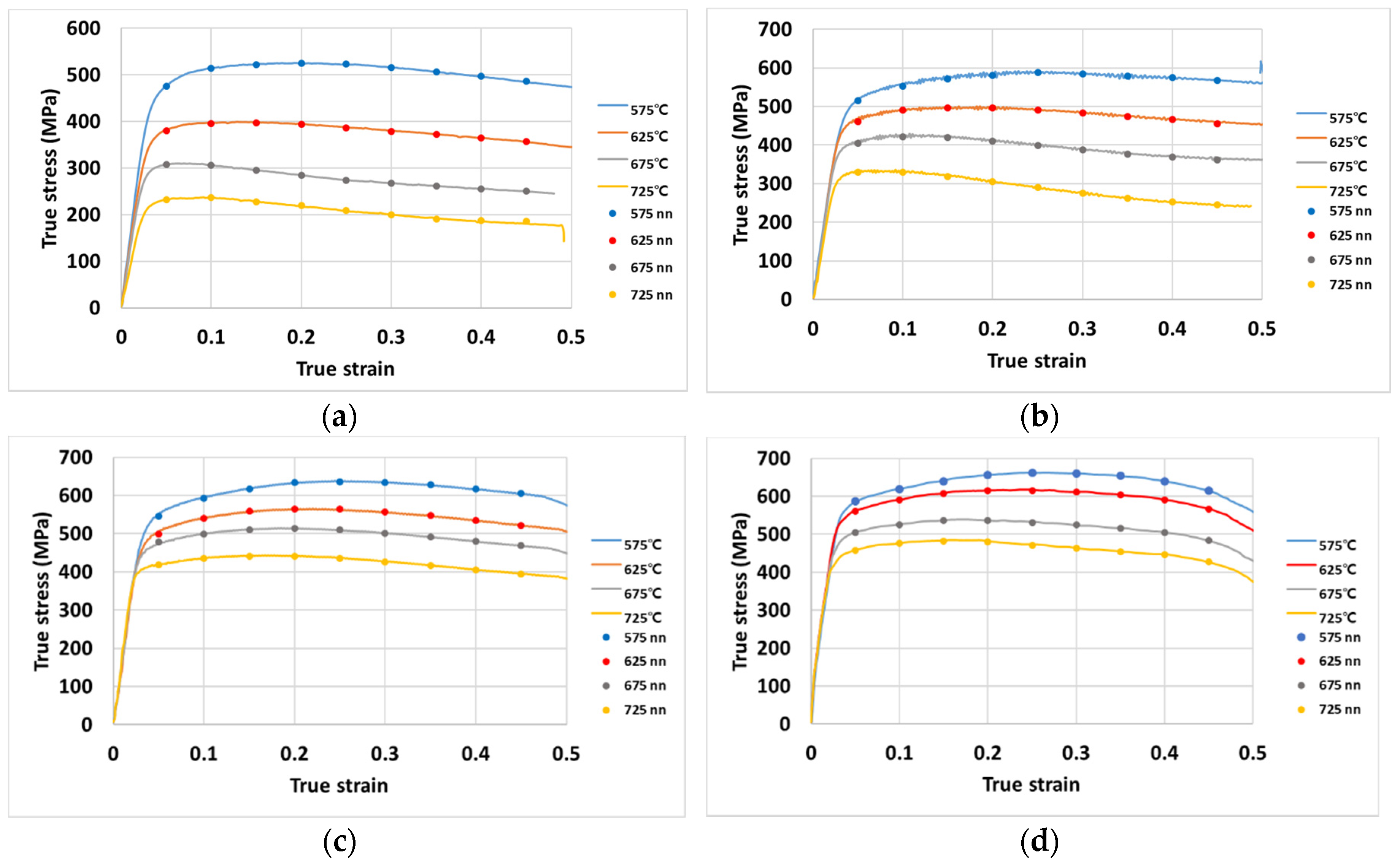
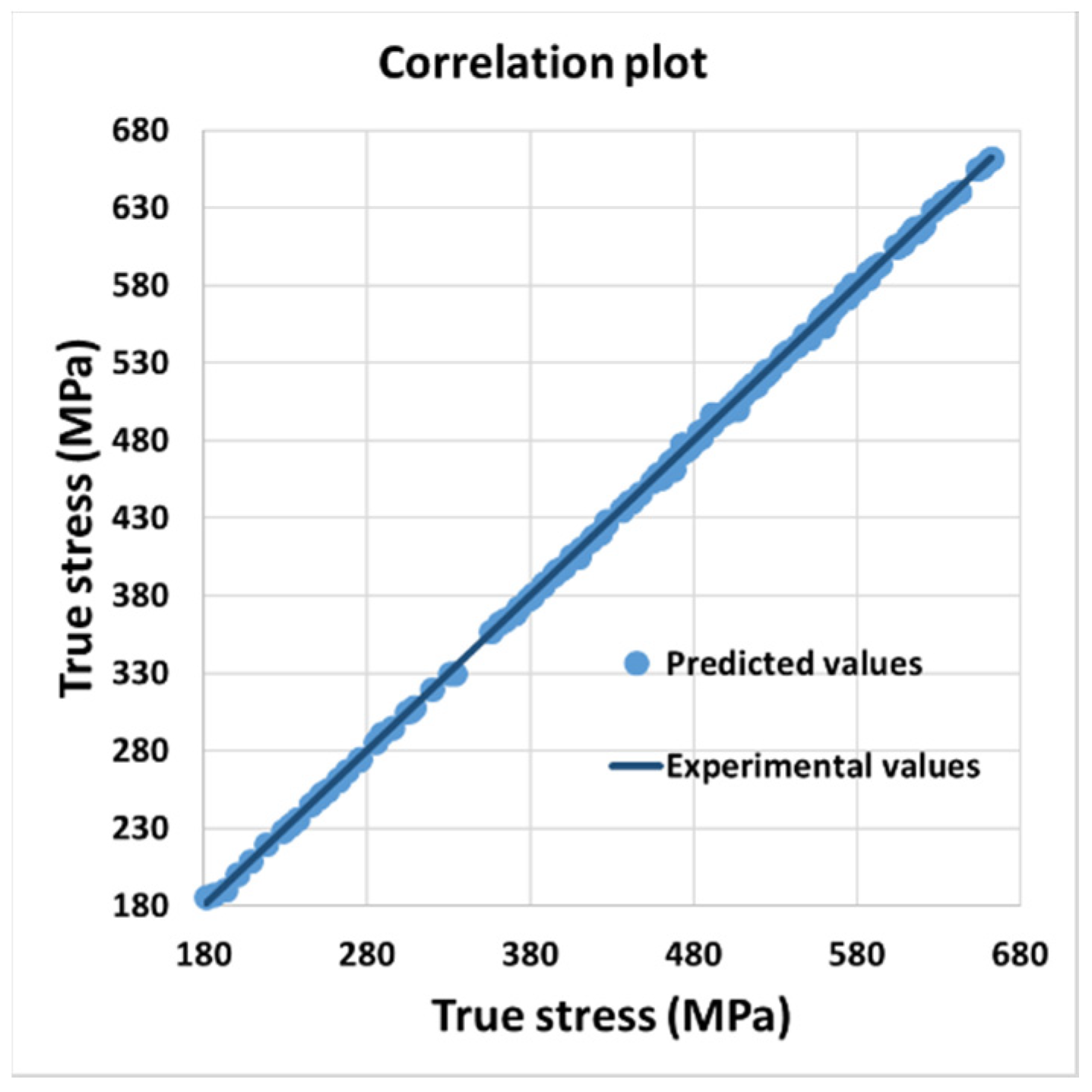
Figure 7 shows the stress–strain curves measured from experiments with predicted stress by the neural network at (a) 0.002 s−1, (b) 0.02 s−1, (c) 2 s−1 and (d) 20 s−1, respectively. The marked neural network predictions showed a good match with the experimental values. The RMSE value of the developed neural network model was 1.87. Figure 8 shows the correlation plot for experimental data and predicted data. In this context, the plot shows that stress calculated by the neural network is much closer to the experimental values. Although the neural network model can calculate the stresses with higher accuracy, the algorithm required more effort to develop and optimize the model, and a longer running time was necessary for the simulations. Hence the neural network model for the current research is computationally costly.
3.3. Decision Tree
Figure 9 represents the stress values marked with the experimental stress–strain curves when the temperature ranged from 575–725 °C and strain rate is 0.002 s−1, 0.02 s−1, 0.2 s−1, 2 s−1 and 20 s−1. The RMSE for the decision tree prediction was 1.37. In terms of a computational cost, the decision tree modeling needed less work in modeling and optimization of the model, and the computation time was also much lower.
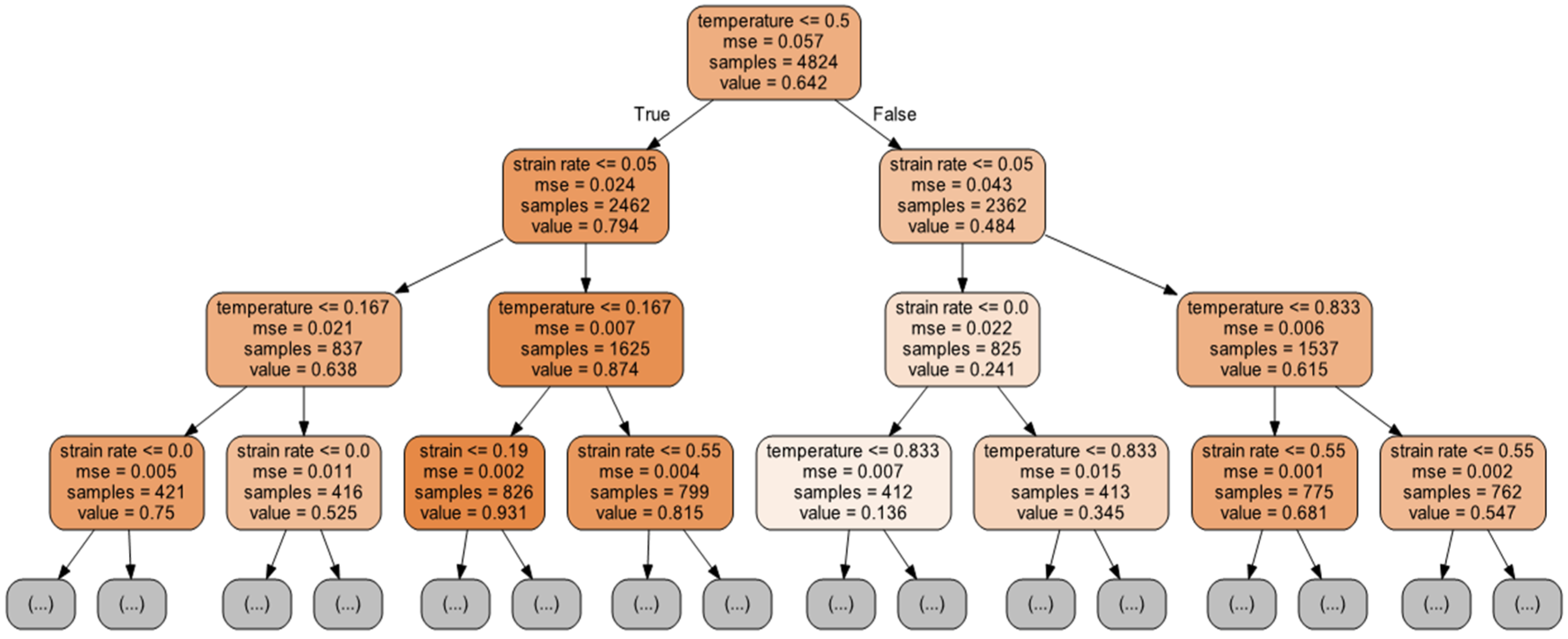
Figure 10 is the part of the decision tree structure for the current model.
Table 4 shows the RMSE for the results predicted by an Arrhenius equation, neural network model and a decision tree algorithm. The result predicted by the Arrhenius equation had the highest RMSE while the results predicted by the neural network model and decision tree algorithm-based model were similar.
4. Conclusions
In this research, hot deformation experiments for Ti-6Al-4V were performed and the flow stresses were modeled by an Arrhenius equation, neural network, and a decision tree algorithm. The following conclusions were drawn:
- -
- A neural network approach and decision tree can predict flow stress with greater accuracy than a traditional Arrhenius equation. The neural network and decision tree approach have more flexibility in describing the irregular variation of the flow stress at different temperatures and strain rates while the way of prediction by an Arrhenius equation is not flexible.
- -
- While both the neural network model and decision tree model can accurately predict the flow stress, the decision tree model is superior to the neural network model in developing efficiency. Performance of the neural network model largely depends on process parameters and resolution algorithms. In addition, optimization work of a neural network model with process parameters takes a relatively long time. In constrast, a decision tree approach takes less time to develop.
- -
- The decision tree approach is computationally inexpensive to utilize and achieves satisfactory results, while calculation of a neural network model takes a relatively long time.
- -
- However, a drawback of the decision tree approach was observed in the developed model. Generally, a decision tree algorithm is known as not being effective in extrapolating the prediction values outside the training dataset. Similar characteristics of the decision tree algorithm is also observed in this research. While the decision tree model could predict the stress for different strains at trained values of temperature and strain rates very accurately, the decision tree model could not predict the flow stress for the temperatures and strain rates other than trained ones.
Author Contributions
Conceptualization, S.-H.S.; methodology, S.-S.L. and S.-H.S.; software, S.-H.S.; validation, S.-H.S.; formal analysis, S.-H.S.; investigation, S.-H.S.; resources, S.-S.L.; data curation, S.-S.L. and S.-H.S.; writing—original draft preparation, S.-H.S.; writing—review and editing, S.-S.L., H.-J.L. and S.-H.S.; visualization, S.-H.S.; supervision, S.-H.S.; project administration, S.-S.L. and S.-H.S.; All authors have read and agreed to the published version of the manuscript.
Funding
This research received no external funding.
Conflicts of Interest
The authors declare no conflict of interest.
References
- Wen, T.; Yue, Y.W.; Liu, L.T.; Yu, J.M. Evaluation and prediction of hot rheological properties of Ti-6Al-4V in dual-phase region using processing map and artificial neural network. Indian J. Eng. Mater. Sci. 2014, 21, 647–656. [Google Scholar]
- Nguyen, D.T.; Kim, Y.S.; Jung, D.W. Flow stress equations of Ti-6Al-4V titanium alloy sheet at elevated temperatures. Int. J. Precis. Eng. Man 2012, 13, 747–751. [Google Scholar] [CrossRef]
- Cai, J.; Li, F.; Liu, T.; Chen, B.; He, M. Constitutive equations for elevated temperature flow stress of Ti–6Al–4V alloy considering the effect of strain. Mater. Des. 2011, 32, 1144–1151. [Google Scholar] [CrossRef]
- Inagaki, I.; Takechi, T.; Shirai, Y.; Ariyasu, N. Application and features of titanium for the aerospace industry. Nippon Steel Sumitomo Met. Tech. Rep. 2014, 106, 22–27. [Google Scholar]
- Fujii, H.; Takahashi, K.; Yamashita, Y. Application of titanium and its alloys for automobile parts. Shinnittetsu Giho 2003, 62–67. [Google Scholar]
- Costan, A.; Dima, A.; Ioniţă, I.; Forna, N.; Perju, M.C.; Agop, M. Thermal properties of a Ti-6AL-4V alloy used as dental implant material. Optoelectron Adv. Mat. 2011, 5, 92–95. [Google Scholar]
- Beal, J.D.; Boyer, R.; Sanders, D.; Company, T.B. Forming of titanium and titanium alloys. ASM Handb. Metalwork. Sheet Form. 2006, 14B, 656–669. [Google Scholar] [CrossRef]
- Kopec, M.; Wang, K.; Wang, Y.; Wang, L.; Lin, J. Feasibility study of a novel hot stamping process for Ti6Al4V alloy. MATEC Web. Conf. 2018, 190, 08001. [Google Scholar] [CrossRef] [Green Version]
- Zamzuri, H.; Ken-Ichiro, M.; Tomoyoshi, M.; Yuya, Y. Hot stamping of titanium alloy sheet using resistance heating. Vestnik Nosov Magnitogorsk State Tech. Univ. 2013, 5, 12–15. [Google Scholar]
- Porntadawit, J.; Uthaisangsuk, V.; Choungthong, P. Modeling of flow behavior of Ti–6Al–4V alloy at elevated temperatures. Mater. Sci. Eng. A 2014, 599, 212–222. [Google Scholar] [CrossRef]
- Zhang, C.; Li, X.Q.; Li, D.S.; Jin, C.H.; Xiao, J.J. Modelization and comparison of Norton-Hoff and Arrhenius constitutive laws to predict hot tensile behavior of Ti–6Al–4V alloy. Trans. Nonferrous Met. Soc. China 2012, 22, 457–464. [Google Scholar] [CrossRef]
- Bruschi, S.; Poggio, S.; Quadrini, F.; Tata, M.E. Workability of Ti–6Al–4V alloy at high temperatures and strain rates. Mater. Lett. 2004, 58, 3622–3629. [Google Scholar] [CrossRef]
- Sabokpa, O.; Zarei-Hanzaki, A.; Abedi, H.R.; Haghdadi, N. Artificial neural network modeling to predict the high temperature flow behavior of an AZ81 magnesium alloy. Mater. Des. 2012, 39, 390–396. [Google Scholar] [CrossRef]
- Zhao, J.; Ding, H.; Zhao, W.; Huang, M.; Wei, D.; Jiang, Z. Modelling of the hot deformation behaviour of a titanium alloy using constitutive equations and artificial neural network. Comput. Mater. Sci. 2014, 92, 47–56. [Google Scholar] [CrossRef]
- Quan, G.Z.; Yu, C.T.; Liu, Y.Y.; Xia, Y.F. A comparative study on improved arrhenius-type and artificial neural network models to predict high-temperature flow behaviors in 20MnNiMo alloy. Sci. World J. 2014, 2014, 108492. [Google Scholar] [CrossRef] [PubMed]
- Sun, Y.; Hu, L.; Ren, J. Modeling the constitutive relationship of powder metallurgy Ti-47Al-2Nb-2Cr alloy during hot deformation. J. Mater. Eng. Perform. 2015, 24, 1313–1321. [Google Scholar] [CrossRef]
- Rahmaan, T.; Abedini, A.; Butcher, C.; Pathak, N.; Worswick, M.J. Investigation into the shear stress, localization and fracture behaviour of DP600 and AA5182-O sheet metal alloys under elevated strain rates. Int. J. Impact Eng. 2017, 108, 303–321. [Google Scholar] [CrossRef]
- Butcher, C.; Abedini, A. Shear confusion: Identification of the appropriate equivalent strain in simple shear using the logarithmic strain measure. Int. J. Mech. Sci. 2017, 134, 273–283. [Google Scholar] [CrossRef]
- Kotsiantis, S.B. Decision trees: A recent overview. Artif. Intell. Rev. 2013, 39, 261–283. [Google Scholar] [CrossRef]
Figure 1.
Compression test. (a) Mounted specimen and (b) hot compression process.

Figure 2.
Schedule of isothermal hot compression test.

Figure 3.
True stress–true strain curves at: (a) 0.002/s; (b) 0.02/s; (c) 2/s; (d) 20/s.

Figure 4.
Structure of neural network.

Figure 5.
Schematic diagram of decision tree algorithm.

Figure 6.
Predicted stress by Arrhenius equation at: (a) 0.002/s; (b) 0.02/s; (c) 2/s; (d) 20/s

Figure 7.
Predicted stress by neural network model at: (a) 0.002 s−1; (b) 0.02 s−1; (c) 2 s−1; (d) 20 s−1.
Figure 7.
Predicted stress by neural network model at: (a) 0.002 s−1; (b) 0.02 s−1; (c) 2 s−1; (d) 20 s−1.

Figure 8.
Experimental data (line) vs. predicted data (dots).

Figure 9.
Predicted stress by decision tree modeling at: (a) 0.002 s−1; (b) 0.02 s−1; (c) 2 s−1; (d) 20 s−1.
Figure 9.
Predicted stress by decision tree modeling at: (a) 0.002 s−1; (b) 0.02 s−1; (c) 2 s−1; (d) 20 s−1.

Figure 10.
Decision tree for the current model.


Table 1.
Parameters for the neural network model.
| Parameter | Input Neurons | Neurons in Hidden Layers | Output Neuron | Epochs | Learning Rate | Weight Decay |
|---|---|---|---|---|---|---|
| Value | 3 | 85, 85 | 1 | 1500 | 0.001 | 0.1 |
Table 2.
Parameters for decision tree model.
| Parameter | Input Attributes | Depth of the Tree | Min. Number of Samples Required to Split an Internal Node | Min. Number of Samples Required to be at a Leaf Node |
|---|---|---|---|---|
| Value | 3 | Unlimited | 2 | 1 |
Table 3.
Parameters for Arrhenius equation.
| 0.05 | 0.1 | 0.15 | 0.2 | 0.25 | 0.3 | 0.35 | 0.4 | 0.45 | |
| 0.00246 | 0.00238 | 0.00236 | 0.00238 | 0.00242 | 0.00247 | 0.00252 | 0.00259 | 0.00269 | |
| n | 17.234 | 16.36 | 14.925 | 13.865 | 13.228 | 12.899 | 12.634 | 12.5 | 12.958 |
| Q | 445.811 | 479.226 | 476.591 | 478.711 | 490.718 | 501.827 | 506.973 | 511.547 | 540.787 |
| Z | 5.79215 × 1024 | 6.62559 × 1026 | 4.55896 × 1026 | 6.15814 × 1026 | 3.38165 × 1027 | 1.63453 × 1028 | 3.3915 × 1028 | 6.48913 × 1028 | 4.10524 × 1030 |
Table 4.
Root mean square error comparison for three approach.
| Arrhenius Equation | Neural Network Model | Decision Tree |
|---|---|---|
| 36.72 | 1.87 | 1.37 |
© 2020 by the authors. Licensee MDPI, Basel, Switzerland. This article is an open access article distributed under the terms and conditions of the Creative Commons Attribution (CC BY) license (http://creativecommons.org/licenses/by/4.0/).
Share and Cite
MDPI and ACS Style
Lim, S.-S.; Lee, H.-J.; Song, S.-H. Flow Stress of Ti-6Al-4V during Hot Deformation: Decision Tree Modeling. Metals 2020, 10, 739. https://doi.org/10.3390/met10060739
AMA Style
Lim S-S, Lee H-J, Song S-H. Flow Stress of Ti-6Al-4V during Hot Deformation: Decision Tree Modeling. Metals. 2020; 10(6):739. https://doi.org/10.3390/met10060739
Chicago/Turabian StyleLim, Seong-Sik, Hye-Jin Lee, and Shin-Hyung Song. 2020. "Flow Stress of Ti-6Al-4V during Hot Deformation: Decision Tree Modeling" Metals 10, no. 6: 739. https://doi.org/10.3390/met10060739
Note that from the first issue of 2016, this journal uses article numbers instead of page numbers. See further details here.