Effects of Uncertainty Shocks on Household Consumption and Working Hours: A Fuzzy Cognitive Map-Based Approach


1
Department of Economics, Seoul National University, Seoul 08826, Korea
2
Department of Applied Mathematics, Hanyang University, Gyeonggi 15588, Korea
*
Author to whom correspondence should be addressed.
Mathematics 2020, 8(6), 889; https://doi.org/10.3390/math8060889
Submission received: 8 May 2020
/
Revised: 21 May 2020
/
Accepted: 25 May 2020
/
Published: 2 June 2020
(This article belongs to the Special Issue Applications of Mathematical Methods and Fuzzy Techniques in Decision Making)
Abstract
:This paper aims to model an individual’s decision-making process in relation to macroeconomic dynamics that involve a large number of variables, which might inflict dimensionality issue in empirical analysis. We employ the fuzzy cognitive map (FCM) for this purpose, and present a parsimonious approach in assessing the impacts of uncertainty shocks on individual households by constructing FCM where households adjust their consumption and working hours in response to changes in exogenous economic uncertainty. We employ FCM to analyze how uncertainty shocks affect the households’ consumption, working hours, and income sources. We further conduct simulations to examine roles of expansionary fiscal policy in alleviating the negative impacts of uncertainty shocks. Our simulations yield similar results as compared to the existing literature on the impacts of uncertainty shocks. We suggest a hybrid algorithm of constructing FCM, and hence demonstrate the extensibility of FCM in analyzing complex macroeconomic systems.
1. Introduction
Fuzzy cognitive map (FCM) has been widely employed as a modeling device to map a person or an entity’s decision-making process with a simple set of monotonic and symmetric causal relations between abstract concepts. In applying this model to analyze socio-economic issues, Calvarho [1] suggests FCM to be used for running scenario simulations and studying system dynamics. FCM’s strength lies in its structural simplicity when resembling a complicated system of economic and social variables. It maps monotonic causal relations between the variables of interest and hence enables a concise computation when assessing various scenarios.
Despite FCM’s strength in simplifying complex systems, its use in terms of modeling macroeconomic dynamics has been limited, though fuzzy logic has been used in assessing financial risks of banks in the existing literature [2]. In this respect, we intend to model an individual’s decision-making process in relation to macroeconomic dynamics, by including a large number of variables in the system. We employ FCM in resembling an economic system and evaluating the changes inflicted by exogenous shocks that occur to the system. Once constructed, FCM can simulate impacts of an exogenous shock on the entire system with many variables. In this regard, FCM enables analysis of changes in a large set of endogenous variables in the system as compared to multivariate models such as vector autoregression (VAR). We find this trait of FCM particularly useful when analyzing the dynamics of a large set of endogenous variables, especially when dynamics of both macro-level and micro-level variables are to be modeled in a single model.
In this light, we particularly study the effects of exogenous uncertainty shocks on household consumption and working hours using both aggregate economic data and household-level data. We design a system in which households adjust their consumption and working hours in response to uncertainty shocks introduced to the economy as a whole. Then, we conduct scenario simulations using the constructed FCMs and assess the results with regard to existing economic literature on macroeconomic effects of uncertainty shocks.
Preceding studies have shown that uncertainty arises from both the financial sector and policy sector, and these shocks are heterogeneous in terms of exogeneity and impact ([3,4,5]). These studies offer sensitivity analyses on macroeconomic dynamics as a whole but do not present much discussion on how the shocks affect individual household’s wealth, income, consumption, and working hours. The reason is obvious. Traditional empirical models on macroeconomic dynamics employ VAR models, and stability of VAR is deteriorated as the model becomes complex with a large number of endogenous variables [6]. Therefore, one might consider using a simpler model to combine an individual household’s decision-making scheme with the macroeconomic system.
This is the reason why we propose to use FCM to analyze how uncertainty shocks affect macroeconomic variables, which in turn affect individual household’s income and wealth, and, as a consequence, the household’s consumption and working hours. In particular, we generate FCM for each household each year. In every map we set, uncertainty indices are assumed to be exogenous and they induce endogenous changes in household’s consumption and working hours. By doing this, we present a parsimonious setting where nationwide uncertainty shocks, coupled with macroeconomic dynamics, affect individual household’s financial status, consumption, and labor supply choices. We exploit the usefulness of our FCM-based approach by assessing scenarios in which exogenous uncertainty shocks occur in the system and see how households’ wealth, income, consumption, and working hours change by comparing them to results from the scenarios without shock.
The paper is organized as follows: we first review existing literature on macroeconomic effects of uncertainty shocks in Section 2 and discuss what FCM is in Section 3. In Section 4, we describe the data and our design of FCM to analyze the data. In Section 5, we evaluate two scenario simulations and offer concluding remarks in Section 6.
2. Literature Review
Effects of uncertainty shocks on the economy has been extensively studied since the seminal work of Bloom [7]. Following Bloom [7], literature on macroeconomic dynamics inflicted by uncertainty shocks mainly discusses measurement and identification of uncertainty shocks and present sensitivity analysis of economic variables in the presence of exogenous shocks. Bloom [7] and Christiano et al. [8] employ financial market volatility as a measure of uncertainty and show that the financial market serves as a transmission channel of the uncertainty shock to real economic variables.
While these studies specify the market uncertainty to originate from the financial sector, Baker et al. [9] proposed to measure the Economic Policy Uncertainty (EPU) index based on media and news analysis. Moreover, Fernàndez-Villaverde et al. [10] specified the fiscal policy as a source of economic uncertainty and conducted an impulse-response analysis of macroeconomic variables. Mumtaz and Theodoridis [6] employed a factor augmented VAR model to estimate the overall economic uncertainty and showed that the impact of uncertainty shocks on macroeconomic variables changed from time to time. These studies, to sum up, mainly focused on tracing the cause of uncertainty to certain economic sectors such as the financial market or the government and incorporated the specification of volatility shocks into the theoretical DSGE framework.
Aside from how macroeconomic variables respond to exogenous uncertainty shocks, lengthy literature exists on how households react to such shocks by changing savings and labor supply. Carroll [11], Carroll et al. [12], and Deaton [13] provide theoretical framework for households’ precautionary saving. Carroll [11] especially focuses on the buffer-stock saving behavior, characterizing that households set target wealth and make saving choices to meet such target. Hence, in times of uncertainty, households’ expected future wealth generally declines, whereas the target wealth remains the same, and thus households increase savings to maintain the expected future wealth. Recent studies also shed some light on precautionary labor supply of households. Since the main source of households’ earnings is labor income, households can increase labor supply to prepare for future income fluctuations and uncertainty. Flodén [14], Pijoan-Mas [15], and Nocetti and Smith [16] show that labor supply choices by households serve as a self-insurance scheme together with saving choices, provided that labor supply can flexibly change in the market. Wu and Krueger [17] also show that households respond to wage shocks by adjusting the labor supply of its members and exploiting its accumulated asset as well. In sum, existing literature on the impacts of uncertainty shocks with respect to household income mainly features changes in household labor supply and savings. In this regard, we construct the FCM in which households change its consumption and working hours in response to economic uncertainty shocks in Section 4.
3. Fuzzy Cognitive Map
Introduced by Kosko [18], FCM is a graphical model that represents causality between variables and concepts. It is fuzzy since it reflects the strength of both positive and negative causal relations that exist between the concepts in inference. The degree of causality is hence represented in a real number in . To be specific, FCM consists of concepts and weights. Concepts could be thought as variables of interest and they could be classified into trigger concepts and output concepts, which are important in decision-making processes. Concepts may be collected from either linguistic data or numerical data, and they are fuzzified into numerical values that represent the degree of their prevalence. Concept values are generally in the range of or . FCM updates these concept values through an iterative procedure until the values converge to certain equilibrium values.
Weights are numerical values that represent causal relations between such variables, of which signs mean either positive or negative causality and values represent the strength of such relation. Weights are typically specified according to experts’ interviews and public polls, and this leads to criticism on using FCM that the inference based on FCM is subjective and ad hoc. However, as Carvalho [1] puts it, FCM takes the specified causal relations to be certain and offer a dynamic propagation of the changes in concepts. Therefore, once the weights are properly assigned, FCM can offer scenario evaluations and dynamics analysis.
After the concept values and weights are assigned and the map is constructed, FCM updates the concept values by an iterative process. Concept values are updated in each iteration, and iterations are run until either the maximum number of iterations is reached or the concept values converge to some constant values.
The updating scheme of FCM could be stated as follows: stands for the value of concept i at n-th iteration, and stands for the weight of concept j on concept i. is a combination of an inference rule and a transformation function defined in the map. Inference rules are defined to calculate the input concept values and the weights into a single value, and that value is put into a transformation function to update the concept values. One may employ various inference rules as in Papageorgiou [19]. Commonly used transformation functions include bivalent, trivalent, sigmoid, and hyperbolic tangent function. When concept values are to be in the interval , sigmoid functions are used in general. If concept values are to be in the interval , hyperbolic tangent functions are used:
Specification of the weights, inference rules, and transformation functions determine whether or not a FCM is stable. By stability, we mean that concept values converge to equilibrium state values after a number of iterations. Boutalis et al. [20] proved existence and uniqueness of such equilibrium values in FCM with sigmoid transformation functions.
To sum up, analyses based on FCM are conducted according to the following steps:
- Step 1. Determine the weights and fuzzify input concept values.
- Step 2. Determine the inference rule and transformation function to be used in FCM inference.
- Step 3. Convert the output concept values into real data values for further analysis.
As could be seen in the steps above, FCM grants much liberty to the researcher in a sense that the researcher can choose fuzzification methods, inference rules, and transformation functions to use. This leads to a critical drawback of FCM that the simulated results from FCM are ad hoc and even more, highly sensitive to tuning parameters that are specified in transformation functions. Thus, finding the optimal tuning parameter is necessary to guarantee the predictability of the constructed FCM. In this study, we use a grid search algorithm to obtain the optimal tuning parameter. The detailed procedure is further discussed in Section 4.
4. Data Analysis
4.1. Data Description
We employ FCM to analyze the effects of uncertainty shocks on individual household’s savings and working hours. Before constructing the map, we introduce the concepts in our FCM and corresponding data. There are 18 concepts in our FCM and they can be classified into four groups. It is notable that employing FCM facilitates specifying the causal relations between these concepts and analyzing dynamics in the system without inflicting much dimensionality issue.
The concepts in our FCM can be classified into following groups: exogenous concepts, macroeconomic concepts, household state concepts, and household choice concepts. Causal effects between the concepts are organized sequentially following the pre-determined exogeneity order: exogenous concepts, macroeconomic concepts, household state concepts, and household choice concepts in the end. We impose such hierarchical structure in the map following existing literature on the effects of uncertainty shocks. Bloom [7], Choi and Shim [4], and Bhattarai et al. [21] all impose the similar identification in each of their VAR models. They impose Cholesky ordering of variables so that the uncertainty shocks instantly affect macroeconomic variables. Similar to their model design, we set uncertainty shock variables as exogenous concepts that affect all other concepts in our FCM.
Our data include 18 variables consisting of 10 aggregate variables and eight household-specific variables. Our data sources are Economic Statistics System (ECOS) provided by Bank of Korea and Korean Labor Income Panel Study (KLIPS). We additionally collect Korean EPU from the website (www.policyuncertainty.com). We collect data from 2006 to 2016 and incorporate macro data with 997 individual household panels.
By exogenous concepts, we mean that these concepts serve as the only force in the FCM that drives changes in other concepts. We specify Financial Stress Index (FSI) presented by Cardarelli et al. [22] and Economic Policy Uncertainty Index (EPU) introduced by Baker et al. [9] as exogenous concepts. We calculate daily FSI based on the methodology proposed by Cardarelli et al. [22] using KOSPI log-return rates, KRW-USD nominal effective exchange rates, and interest rates, and take the annual mean of the index. Then, we use Hodrick–Prescott detrended values of the two indices and identify their deviations as annual uncertainty shocks. We assume that the two shocks cause changes to each other interdependently and they together affect rest of the concepts in the map.
We specify eight macroeconomic concepts, which are affected by exogenous variables and, in turn, change the household characteristic concepts. The macroeconomic concepts are consumer sentiment index, lending attitude index designed by Bank of Korea, household borrowing interest rate, inflation rate, unemployment rate, GDP growth rate, KOSPI index, and government expenditure. All variables are annual values. Specifically, lending attitude index reflects banks’ willingness to make loans to firms and households and is collected from a survey. Household borrowing interest rates are borrowing rates for household new loans. Lastly, we include the detrended government expenditure by using Hodrick–Prescott filtered annual deviations in the map to take account of the government’s fiscal adjustments in response to uncertainty shocks.
We also include six household state concepts that summarize individual household’s financial status and two choice concepts that households adjust based on each of their financial situations. Household state concepts include a household’s debt, asset, labor income, financial income, real estate income, and transfer income. We particularly specify four sources of household income to see if different sources of uncertainty affect the income in different ways. Then, we introduce household annual consumption expenditure and average weekly working hours as the household choice concepts. This is to resemble traditional macroeconomic models where households choose consumption and labor supply given budget constraints. One may point out that household’s working hours are labor market equilibrium values and hence they are different from household labor supply. This is precisely why we include macroeconomic variables such as GDP growth rates and unemployment rates in our cognitive map and control possible effects of labor demand on household working hours. All of these concepts except for working hours are in real terms divided by annual Consumer Price Index, respectively.
To sum up, we include 18 macroeconomic and household specific variables from 2006 to 2016 in our cognitive map analysis. Parsimony of FCM in terms of computation enables us to analyze dynamics and relations between these variables. We further describe how each of these variables are converted into concept values and how causal weights are determined in the following subsection.
4.2. FCM Setting and Inference Scheme
As mentioned before, we study households’ consumption and labor supply decisions by constructing an FCM for each household each year. We include 18 macroeconomic and household-specific concepts in our cognitive map. To initialize the inference procedure, we first standardize the variables and convert them into z scores. For household-specific variables, we standardize the variables each year to reflect each household’s relative positions. We then normalize the z scores into values in by plugging them into sigmoid function: .
We then set the weights that specify causal relations between concepts. As described in the previous section, exogenous concepts cause changes in all other concepts while macroeconomic concepts alter household-specific concepts only. Lastly, household state concepts affect the two household choice concepts, consumption expenditure, and working hours. We do not allow for feedback from the household-specific concepts to macroeconomic and exogenous concepts, and impose no autoregressive structure in the process of exogenous concepts. This is because our aim is to design an FCM that represents the decision-making process of each household each year.
We first assign initial weights upon which we build 10,967 weight matrices in total. We conduct regression of each variable with all other variables one at a time, and then employ the standardized regression coefficients as the initial weights between concepts. We conduct regressions separately for each year, so 11 initial weight matrices are assigned for years 2006 to 2016. We first estimate the following regression:
where is weight of concept j on concept i, i and j are concept indices, and h is household index. We augment values of if the values depart from what the previous studies suggest. Hence, our approach is a hybrid of data-driven and model-driven approaches in terms of designing FCM. A similar, regression-based approach was employed in fuzzy analysis of multiple variables [23].
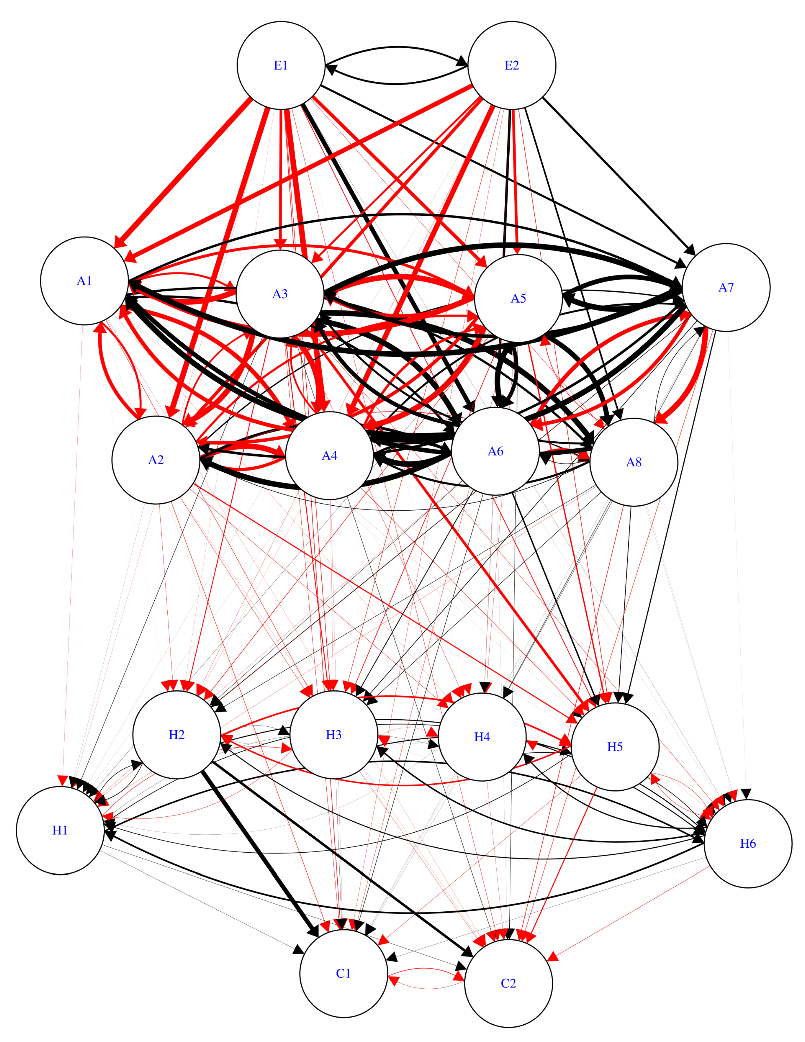
Table 1 is the list of concepts and their labels to be used in Figure 1 and Table 2. Table 2 is the mean of 11 initial weight matrices that we assign to our cognitive map. As could be seen in Table 2, the uncertainty shocks E1 and E2 affect all other concepts in the FCM, though it is surprising that households’ working hours and EPU shocks apparently showed no sign of correlation on data. Effects of uncertainty shocks on each variable matches the conventional wisdom in general, and we set this matrix as the input weight matrix for the weight-updating process.
Figure 1 is a graphical illustration of FCM assigned the mean initial weight matrix. Note that the black and red lines stand for positive and negative causal relation between concepts, respectively. Width of the lines represents the degree of causality, with wider lines drawn for stronger relations.
We update the yearly initial matrices to design FCM for each household via nonlinear Hebbian learning method. We employ the method similar to that proposed by Papageorgiu et al. [24]. Papageorgiu et al. [24] suggest the following scheme to update weights. Weights are updated after each simulation step until the sum of two subsequent output concepts’ differences is smaller than some numerical value as small as . is the weight of concept j on concept i at n-th simulation and is concept value of j at n-th simulation:
We obtain the weight matrix for each household using Equation (4) and then use them to predict the household’s consumption expenditure and working hours in the next year. In actual implementation of FCM inference, we choose the rescale inference rule:
Transformation function is sigmoid function with of 1.3. The value of was selected to maximize the FCM’s in-sample forecasting performance of household consumption expenditure and working hours. We define one iteration step as one year in real time, hence our forecasts of household consumption expenditure and working hours are obtained from the concept values of C1 and C2 after one iteration. A similar forecasting procedure was employed in Gupta and Gupta [25].
We plug the concept values in the inverse function of sigmoid function: to obtain forecasts of household consumption and working hours in the next year. By this, we numerically convert the output concept values into real values. Our overall method is summarized in Algorithm 1.
| Algorithm 1: Forecasting Household Consumption and Weekly Working Hours with FCM |
 |
After we obtain forecasts of household consumption and working hours for every household each year, we compute the root mean squared error (RMSE) of the simulated results and the data. RMSE are reported as 6.981 for real consumption expenditures and 11.113 for weekly working hours. We conclude that our approach offers reasonable forecasts for the two household choice variables.
5. Scenario Analysis
FCM has been proven useful in assessing various scenarios with different sets of input concept values. Employing the FCMs constructed in Section 4, we examine two situations in which 1-SD shock is introduced to the two uncertainty indices and see how household consumption and working hours, as well as other household status variables, respond to uncertainty shocks. We also analyze how expansionary fiscal policy in response to the shocks can alleviate the negative effects of uncertainty shocks on the economy at household level.
5.1. Effects of FSI Shock
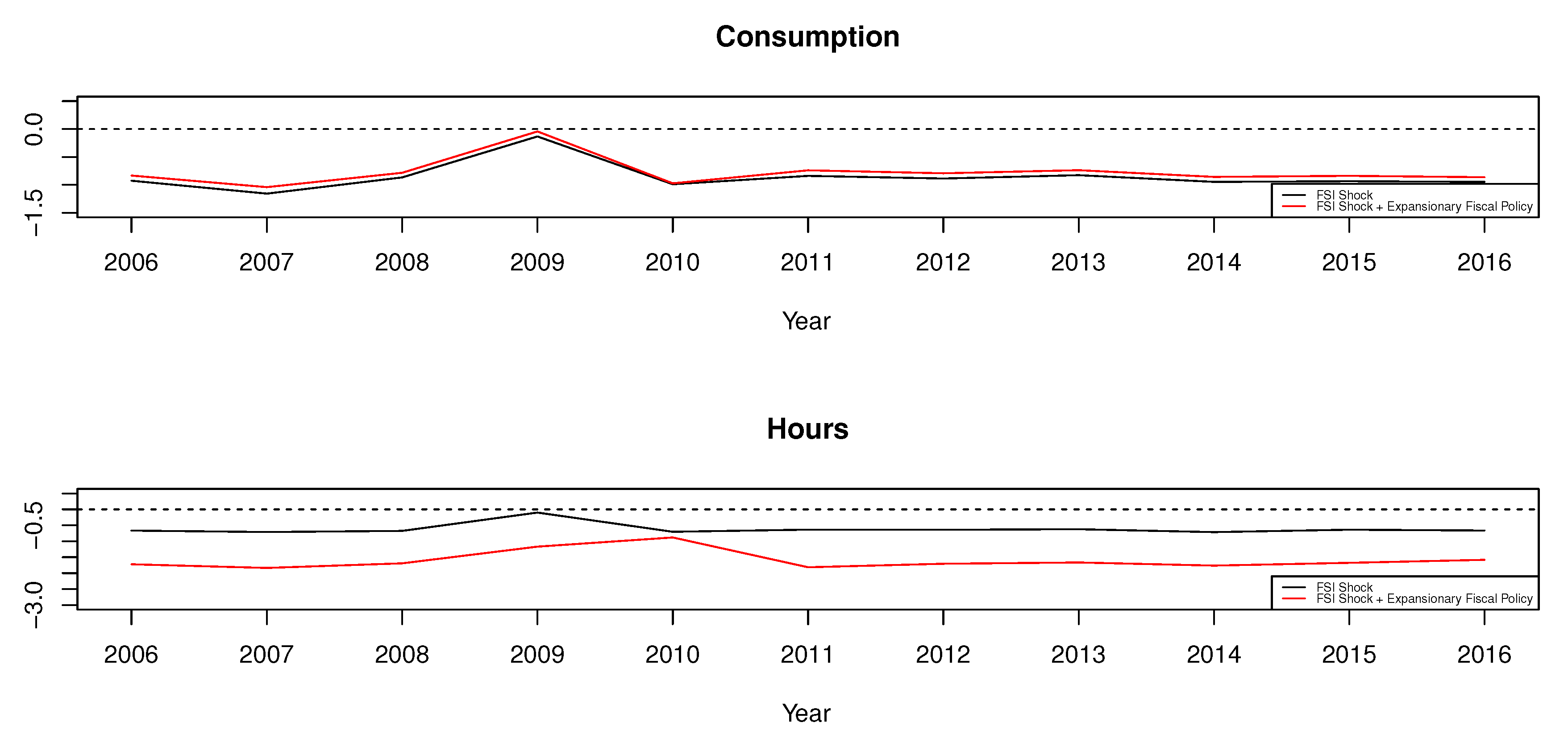
We first examine the situation where FSI increases by one standard deviation each year. We compare the simulated results to those obtained from the simulation in which government expenditure also increases by one standard deviation in response to the uncertainty shocks. We plot average changes in consumption and working hours as annual FSI increases by 1 standard deviation in Figure 2. We observe that 1-SD shock on FSI decreases both household consumption expenditures and working hours in all years throughout 2006 and 2016. Reduction in household consumption could be attributed to a surge in households’ precautionary savings and reduction in income as a result of aggregate dynamics. Household working hours also decrease due to uncertainty shocks because labor demand contracts as uncertainty rises in the market, even if households supply more labor in the market to cover its income losses. Our results are consistent with the estimation of Basu and Bundick [26].
The red lines in Figure 2 are average changes in consumption and working hours as the government increases its expenditure by one standard deviation in response to the uncertainty shocks. We see that the expansionary fiscal policy in times of uncertainty shocks slightly lessens the impact of shock on consumption, but working hours decrease more as the government increases its expenditure. This could be attributed to the fact that increase in government expenditures increases households’ income. This slightly compensates the decrease in households’ consumption but weakens the households’ incentive to participate in the labor market to provide itself with self insurance. In other words, expansionary fiscal policy increases consumption by a small amount but induces income effect on the households’ labor supply.
This is captured in changes in household-specific variables summarized as time-means in Table 3. As the government increases expenditures, household income increases significantly. Households’ financial income (H2) decreases without the expansionary fiscal policy on average, but such decrease is not observed in the simulation with the expansionary fiscal policy. Similar patterns are observed in other sources of income including labor income (H3), real estate income (H4), and transfer income (H5). Hence, the expansionary fiscal policy offsets the impacts of uncertainty shocks by increasing the household income, and the households consume more, work less, and repay more debt (H1) as compared to the situation without any government policy. One puzzling result is that the households’ assets are reported to increase in both simulations, and this implies there is a room for further improvements in our FCM construction.
5.2. Effects of EPU Shock
We conduct a similar exercise by assuming a 1-SD shock on the EPU index. We plot average changes in household consumption and working hours due to EPU shocks in Figure 3. We observe that both consumption and working hours fall due to EPU shocks in this case as well. Moreover, we observe that both consumption and working hours increase as economic policy uncertainty rises in 2009 and 2015, which necessitates further investigations on the transmission mechanisms of EPU shocks in the aggregate economy and a better tuning of our FCM inference. Apart from that, the simulated results obtained from the scenario with EPU shocks exhibit similar trends with those from the scenario with FSI shocks.
Simulated effects of EPU shocks coupled with expansionary fiscal policy are similar to those of FSI shocks with expansionary fiscal policy. Consumption expenditures diminish less while working hours plummet. We also confirm a similar pattern of changes in household-specific variables in Table 4 as compared to Table 3. Though the responses of the variables are more volatile throughout the whole period, household variables respond similarly to the shocks in EPU and expansionary fiscal policy following the shocks.
Hence, from Table 3 and Table 4, we conclude that the FCM we constructed in Section 4 adequately captures macroeconomic dynamics as well as their impacts on the household variables including consumption and working hours choices. Though it seems that further adjustments could be made upon our FCM to make household debt and assets evolve in a more plausible way, our FCM is sufficient in offering a parsimonious summary of the impacts of uncertainty shocks on the economy as a whole and, at the same time, on the households on an individual level.
6. Conclusions
We study the effects of two different types of uncertainty shocks on household consumption and working hours by constructing FCM for 997 Korean households from 2006 to 2016. In doing so, we identify macroeconomic uncertainty stemming from financial instability and economic policies and hence employ the financial stress index (FSI) and the economic policy uncertainty (EPU) as proxies of uncertainty. We construct an FCM in which shocks on these two uncertainty indices first affect the macroeconomic variables and consequently the household specific variables. After generating FCM for each household from the initial FCM, we analyze how household consumption and working hours, as well as other household status variables, are affected by exogenous uncertainty shocks. We also examine how expansionary fiscal policy can alleviate negative effects of such shocks on households.
The two types of uncertainty shocks affect the households in similar ways, though the impacts of EPU shocks are more volatile across the whole period. Uncertainty shocks reduce both consumption expenditures and working hours in our simulations, in similar magnitudes. When the government increases expenditures to combat the negative effects of shocks, our simulations present that decreases in consumption expenditures are lessened, whereas working hours shrink even more. This happens because the expansionary fiscal policy compensates household income and consequently induces income effect on households’ labor supply choices in our simulations.
Our FCM-based approach on analyzing effects of uncertainty shocks on the aggregate economy and individual households simplifies the complicated macroeconomic dynamics implied in the original data. It also incorporates both macroeconomic data and individual data successfully, so that we can assess micro-effects of uncertainty shocks on individual economic agents. Though our FCM design yields some room of improvements in forecasting changes in household debt and assets, this is rather the flexibility of our approach, since weights assigned to FCM can be easily modified. In summary, our approach exemplifies the malleability of FCM in studying more complex socio-economic systems with high-dimensional data. In our further studies, we intend to incorporate a data generating process of exogenous variables to the FCM framework to model an individual’s dynamic decision-making process.
Author Contributions
Conceptualization, Y.Y. and H.-Y.J.; methodology, H.-Y.J.; software, Y.Y.; validation, Y.Y. and H.-Y.J.; formal analysis, Y.Y.; investigation, H.-Y.J.; resources, Y.Y.; data curation, Y.Y.; writing—original draft preparation, Y.Y.; writing—review and editing, H.-Y.J.; visualization, Y.Y.; supervision, H.-Y.J.; project administration, H.-Y.J.; funding acquisition, Y.Y. and H.-Y.J. All authors have read and agreed to the published version of the manuscript.
Funding
This research was supported by Basic Science Research Program through the National Research Foundation of Korea (NRF) funded by the Ministry of Education (NRF-2019R1I1A1A01046810). This research was also supported by the BK21Plus Program (Future-oriented innovative brain raising type, NRF-21B20130000013) funded by the Ministry of Education (MOE, Korea) and the National Research Foundation of Korea (NRF).
Acknowledgments
The authors thank Hyunik Kim of Department of Computer Science and Engineering, Seoul National University, Korea, for his technical support and administration arrangements.
Conflicts of Interest
The authors declare no conflict of interest. The funders had no role in the design of the study; in the collection, analyses, or interpretation of data; in the writing of the manuscript, or in the decision to publish the results.
Abbreviations
The following abbreviations are used in this manuscript:
| FCM | Fuzzy Cognitive Map |
| FSI | Financial Stress Index |
| EPU | Economic Policy Uncertainty |
| VAR | Vector Autoregression |
| DSGE | Dynamic Stochastic General Equilibrium |
References
- Carvalho, J.P. On the semantics and the use of fuzzy cognitive maps and dynamic cognitive maps in social sciences. Fuzzy Sets Syst. 2013, 124, 6–19. [Google Scholar] [CrossRef]
- Sanchez-Roger, M.; Oliver-Alfonso, M.D.; Sanchis-Pedregosa, C. Fuzzy logic and its uses in finance: A systematic review exploring its potential to deal with banking crises. Mathematics 2019, 7, 1091. [Google Scholar] [CrossRef] [Green Version]
- Ludvigson, S.C.; Ma, S.; Ng, S. Uncertainty and business cycles: Exogenous impulse or endogenous response? Am. Econ. J. Macroecon. 2020. forthcoming. [Google Scholar]
- Choi, S.; Shim, M. Financial vs. policy uncertainty in emerging market economies. Open Econ. Rev. 2019, 30, 297–318. [Google Scholar] [CrossRef]
- Stockhammar, P.; Österholm, P. The impact of US uncertainty shocks on small open economies. Open Econ. Rev. 2017, 28, 347–368. [Google Scholar] [CrossRef] [Green Version]
- Mumtaz, H.; Theodoridis, K. The changing transmission of uncertainty shocks in the U.S. J. Bus. Econ. Stat. 2018, 36, 239–252. [Google Scholar] [CrossRef]
- Bloom, N. The impact of uncertainty shocks. Econometrica 2009, 77, 623–685. [Google Scholar]
- Christiano, L.J.; Motto, R.M.; Rostagno, M. Risk shocks. Am. Econ. Rev. 2014, 104, 27–65. [Google Scholar] [CrossRef]
- Baker, S.R.; Bloom, N.; Davis, S.J. Measuring economic policy uncertainty. Q. J. Econ. 2016, 131, 1593–1636. [Google Scholar] [CrossRef]
- Fernández-Villaverde, J.; Guerrón-Quintana, P.; Kuester, K.; Rubio-Ramírez, J. Fiscal volatility shocks and economic activity. Am. Econ. Rev. 2015, 105, 3352–3384. [Google Scholar] [CrossRef] [Green Version]
- Carroll, C.D. Buffer-stock saving and the life cycle/permanent income hypothesis. Q. J. Econ. 1997, 112, 1–55. [Google Scholar] [CrossRef]
- Carroll, C.D.; Hall, R.E.; Zeldes, S.P. The buffer-stock theory of saving: Some macroeconomic evidence. Brookings Pap. Econ. Act. 1992, 1992, 61–156. [Google Scholar] [CrossRef] [Green Version]
- Deaton, A. Saving and liquidity constraints. Econometrica 1991, 59, 1221–1248. [Google Scholar] [CrossRef]
- Flodén, M. Labour supply and saving under uncertainty. Econ. J. 2006, 116, 721–737. [Google Scholar] [CrossRef]
- Pijoan-Mas, J. Precautionary savings or working longer hours? Rev. Econ. Dyn. 2006, 9, 326–352. [Google Scholar] [CrossRef] [Green Version]
- Nocetti, D.; Smith, W.T. Precautionary saving and endogenous labor supply with and without intertemporal expected utility. J. Money Credit Bank. 2011, 43, 1475–1504. [Google Scholar] [CrossRef]
- Wu, C.; Krueger, D. Consumption insurance against wage risk: Family labor supply and optimal progressive income taxation. Am. Econ. J. Macroecon. 2020. forthcoming. [Google Scholar]
- Kosko, B. Fuzzy cognitive maps. Int. J. Man-Mach. Stud. 1986, 24, 65–75. [Google Scholar] [CrossRef]
- Papageorgiou, E.I. Methods and algorithms for fuzzy cognitive map-based modeling. In Fuzzy Cognitive Maps for Applied Sciences and Engineering; Papageorgiou, E.I., Ed.; Springer: Berlin, Germany, 2014; pp. 1–28. [Google Scholar]
- Boutalis, Y.; Kottas, T.L.; Christodoulou, M. Adaptive estimation of fuzzy cognitive maps with proven stability and parameter convergence. IEEE Trans. Fuzzy Syst. 2009, 17, 874–889. [Google Scholar] [CrossRef]
- Bhattarai, S.; Chatterjee, A.; Park, W.Y. Global spillover effects of US uncertainty. J. Monet. Econ. 2019. forthcoming. [Google Scholar] [CrossRef] [Green Version]
- Cardarelli, R.; Elekdag, S.; Lall, S. Financial stress and economic contractions. J. Financ. Stab. 2011, 7, 78–97. [Google Scholar] [CrossRef]
- Yoon, J.H. Fuzzy mediation analysis. Int. J. Fuzzy Syst. 2020, 22, 338–349. [Google Scholar] [CrossRef]
- Papageorgiou, E.I.; Stylios, C.; Groumpos, P. Fuzzy cognitive map learning based on nonlinear Hebbian rule. In AI 2003: Advances in Artificial Intelligence; Gedeon, T.D., Fung, L.C.C., Eds.; Springer: Berlin, Germany, 2003; pp. 256–268. [Google Scholar]
- Gupta, S.; Gupta, S. Modeling economic system using fuzzy cognitive maps. Int. J. Syst. Assur. Eng. Manag. 2017, 8, 1472–1486. [Google Scholar] [CrossRef]
- Basu, S.; Bundick, B. Uncertainty shocks in a model of effective demand. Econometrica 2017, 85, 937–958. [Google Scholar] [CrossRef]
Figure 1.
FCM with initial weight matrix.

Figure 2.
Effects of FSI Shock on consumption and working hours.

Figure 3.
Effects of EPU shock on consumption and working hours.


Table 1.
List of concepts.
| Label | Concept | Label | Concept |
|---|---|---|---|
| E1 | Financial Stress Index | H1 | Debt |
| E2 | Economic Policy Uncertainty | H2 | Financial Income |
| A1 | Consumer Sentiment Index | H3 | Labor Income |
| A2 | Bank Lending Attitude Index | H4 | Real Estate Income |
| A3 | Household Lending Interest Rate | H5 | Transfer Income |
| A4 | KOSPI | H6 | Asset |
| A5 | Unemployment Rate | C1 | Consumption |
| A6 | Inflation Rate | C2 | Working Hours |
| A7 | GDP Growth Rate | ||
| A8 | Government Expenditure |
Table 2.
Initial weight matrix.
| E1 | E2 | A1 | A2 | A3 | A4 | A5 | A6 | A7 | |
|---|---|---|---|---|---|---|---|---|---|
| E1 | 0 | 0.336 | −1 | −1 | −0.488 | −1 | −0.623 | 0.796 | 0.374 |
| E2 | 0.336 | 0 | −0.815 | −0.591 | −0.352 | −0.920 | −0.498 | 0.463 | 0.393 |
| A1 | 0 | 0 | 0 | −0.368 | −0.364 | −0.800 | −0.523 | 0.430 | 0.435 |
| A2 | 0 | 0 | −0.649 | 0 | −0.304 | −1 | −0.387 | 0.526 | 0.229 |
| A3 | 0 | 0 | −1 | −1 | 0 | −1 | −1 | 1 | 1 |
| A4 | 0 | 0 | −0.714 | −0.580 | −0.313 | 0 | −0.449 | 0.428 | 0.343 |
| A5 | 0 | 0 | −1 | −0.615 | −0.643 | −1 | 0 | 0.707 | 0.852 |
| A6 | 0 | 0 | 1 | 1 | 0.730 | 1 | 0.988 | 0 | −0.738 |
| A7 | 0 | 0 | 1 | 0.459 | 0.674 | 1 | 1 | −0.663 | 0 |
| A8 | 0 | 0 | 0.808 | 0.100 | 0.359 | 0.381 | −0.100 | 0.100 | 0.100 |
| H1 | 0 | 0 | 0 | 0 | 0 | 0 | 0 | 0 | 0 |
| H2 | 0 | 0 | 0 | 0 | 0 | 0 | 0 | 0 | 0 |
| H3 | 0 | 0 | 0 | 0 | 0 | 0 | 0 | 0 | 0 |
| H4 | 0 | 0 | 0 | 0 | 0 | 0 | 0 | 0 | 0 |
| H5 | 0 | 0 | 0 | 0 | 0 | 0 | 0 | 0 | 0 |
| H6 | 0 | 0 | 0 | 0 | 0 | 0 | 0 | 0 | 0 |
| C1 | 0 | 0 | 0 | 0 | 0 | 0 | 0 | 0 | 0 |
| C2 | 0 | 0 | 0 | 0 | 0 | 0 | 0 | 0 | 0 |
| A8 | H1 | H2 | H3 | H4 | H5 | H6 | C1 | C2 | |
| E1 | −0.055 | −0.020 | −0.015 | −0.090 | −0.006 | −0.134 | 0.023 | −0.098 | −0.058 |
| E2 | 0.288 | 0.011 | −0.034 | −0.071 | −0.031 | −0.091 | 0.011 | −0.039 | 0 |
| A1 | 0.409 | −0.023 | −0.003 | −0.071 | −0.023 | 0.007 | 0.011 | −0.010 | −0.023 |
| A2 | −0.115 | 0.014 | −0.046 | −0.053 | −0.058 | −0.196 | −0.008 | −0.073 | −0.018 |
| A3 | 1 | 0.079 | −0.149 | −0.153 | −0.050 | −0.479 | −0.055 | −0.060 | 0.069 |
| A4 | 0.172 | 0.010 | −0.019 | −0.024 | −0.004 | −0.073 | 0.002 | −0.021 | −0.005 |
| A5 | 0.894 | 0.034 | −0.091 | −0.113 | −0.037 | −0.226 | 0.002 | −0.050 | 0.066 |
| A6 | −0.465 | −0.028 | 0.061 | 0.140 | 0.018 | 0.251 | −0.012 | 0.080 | 0.009 |
| A7 | −1 | −0.034 | 0.095 | 0.115 | 0.072 | 0.191 | 0.005 | 0.018 | −0.072 |
| A8 | 0 | −0.032 | 0.074 | 0.084 | 0.051 | 0.125 | −0.012 | 0.010 | −0.092 |
| H1 | 0 | 0 | 0.099 | −0.079 | 0.030 | 0.116 | 0.280 | 0.041 | 0.050 |
| H2 | 0 | 0.108 | 0 | 0.036 | −0.005 | −0.299 | 0.174 | 0.779 | 0.452 |
| H3 | 0 | −0.058 | 0.024 | 0 | −0.021 | −0.008 | 0.177 | 0.031 | −0.042 |
| H4 | 0 | 0.017 | −0.002 | −0.016 | 0 | −0.007 | 0.107 | 0.019 | −0.030 |
| H5 | 0 | 0.112 | −0.266 | −0.010 | −0.0119 | 0 | −0.057 | −0.051 | −0.180 |
| H6 | 0 | 0.305 | 0.173 | 0.260 | 0.210 | −0.064 | 0 | 0.030 | −0.063 |
| C1 | 0 | 0 | 0 | 0 | 0 | 0 | 0 | 0 | −0.101 |
| C2 | 0 | 0 | 0 | 0 | 0 | 0 | 0 | −0.048 | 0 |
Note: Element denotes effects of i-th concept on j-th concept.
Table 3.
Effects of FSI shock on household variables.
| No Expansionary Policy | Expansionary Policy | |
|---|---|---|
| C1 | −0.8591 | −0.7728 |
| (0.2451) | (0.2469) | |
| C2 | −0.6149 | −1.5915 |
| (0.1655) | (0.2821) | |
| H1 | −0.7339 | −1.7984 |
| (0.2637) | (0.5070) | |
| H2 | −0.0369 | 0.0000 |
| (0.0117) | (0.0182) | |
| H3 | −0.2337 | 0.9146 |
| (0.0640) | (0.3195) | |
| H4 | −0.0122 | 0.1108 |
| (0.0093) | (0.0760) | |
| H5 | −0.0830 | −0.0032 |
| (0.0348) | (0.0380) | |
| H6 | 0.9234 | 0.4678 |
| (0.3003) | (0.2897) |
Note: Values in parentheses are standard deviations.
Table 4.
Effects of EPU shock on household variables.
| No Expansionary Policy | Expansionary Policy | |
|---|---|---|
| C1 | −0.8577 | −0.7715 |
| (0.8807) | (0.8824) | |
| C2 | −0.6144 | −1.5901 |
| (0.6163) | (0.6403) | |
| H1 | −0.7482 | −1.8111 |
| (0.7970) | (0.8871) | |
| H2 | −0.0306 | 0.0066 |
| (0.0374) | (0.0542) | |
| H3 | −0.2253 | 0.9232 |
| (0.2313) | (0.4279) | |
| H4 | −0.0110 | 0.1133 |
| (0.0125) | (0.0798) | |
| H5 | −0.0651 | 0.0132 |
| (0.0929) | (0.1164) | |
| H6 | 0.8641 | 0.4094 |
| (0.9480) | (0.9955) |
Note: Values in parentheses are standard deviations.
© 2020 by the authors. Licensee MDPI, Basel, Switzerland. This article is an open access article distributed under the terms and conditions of the Creative Commons Attribution (CC BY) license (http://creativecommons.org/licenses/by/4.0/).
Share and Cite
MDPI and ACS Style
Yun, Y.; Jung, H.-Y. Effects of Uncertainty Shocks on Household Consumption and Working Hours: A Fuzzy Cognitive Map-Based Approach. Mathematics 2020, 8, 889. https://doi.org/10.3390/math8060889
AMA Style
Yun Y, Jung H-Y. Effects of Uncertainty Shocks on Household Consumption and Working Hours: A Fuzzy Cognitive Map-Based Approach. Mathematics. 2020; 8(6):889. https://doi.org/10.3390/math8060889
Chicago/Turabian StyleYun, Yeonggyu, and Hye-Young Jung. 2020. "Effects of Uncertainty Shocks on Household Consumption and Working Hours: A Fuzzy Cognitive Map-Based Approach" Mathematics 8, no. 6: 889. https://doi.org/10.3390/math8060889
Note that from the first issue of 2016, this journal uses article numbers instead of page numbers. See further details here.