An Investigation on a Closed-Loop Supply Chain of Product Recycling Using a Multi-Agent and Priority Based Genetic Algorithm Approach

Abstract

Product recycling issues have gained increasing attention in many industries in the last decade due to a variety of reasons driven by environmental, governmental and economic factors. Closed-loop supply chain (CLSC) models integrate the forward and reverse flow of products. Since the optimization of these CLSC models is known to be NP-Hard, competition on optimization quality in terms of solution quality and computational time becomes one of the main focuses in the literature in this area. A typical six-level closed-loop supply chain network is examined in this paper, which has great complexity due to the high level of echelons. The proposed solution uses a multi-agent and priority based approach which is embedded within a two-stage Genetic Algorithm (GA), decomposing the problem into (i) product flow, (ii) demand allocation and (iii) pricing bidding process. To test and demonstrate the optimization quality of the proposed algorithm, numerical experiments have been carried out based on the well-known benchmarking network. The results prove the reliability and efficiency of the proposed approach compared to LINGO and the benchmarking algorithm discussed in the literature.

1. Introduction

The closed-loop supply chain (CLSC) has become more popular in recent years due to several reasons. One of the most prominent reasons is that environmental issues have gained increasing attention. European regulations have increased a producer’s responsibility in several branches of industry, such as WEEE (waste electrical and electronic equipment) 2001 for consumer electronics [1]. Customers also expect to trade-in old products when buying new ones, making producers pay more attention to the reversion of used products or materials. Another crucial reason for operating in the CLSC is the cost. A well-designed CLSC network can provide significant cost savings in procurement, inventory, transportation and recovery processing. Hewlett-Packard estimated that the cost of returns was as much as 2% of their gross outbound sales [2].

Guide and Van Wassenhove [3] defined closed-loop supply chain management (CLSCM) as the design, control and operation of a system to creat maximum value in the entire life cycle of a product, and dynamically restore value from different types and volumes of returns over time. The management of CLSC describes the discipline of optimizing the delivery of goods, services and information from supplier to customer and simultaneously from customer recovery to supplier [4]. With the same principle as in supply chain management, the goals of closed-loop supply chain management typically include transportation network design, location of manufacture, distribution or dismantling center, product recycling and other efforts to improve cost savings. Location selection and transportation network design are two of the most important fields of CLSCM.

Many research studies related to the recovery of products have been conducted in the filed of the supply chain including both academic and industrial applications. Fleischmann et al. [5] and Wells and Seitz [6] believed that the forward and reverse logistics chains should be combined in operations and the flow of materials to establish a closed-loop supply chain. The practical applications of CLSC can be found in many fields. Krikke, Bloemhof-Ruwaard and Van Wassenhove [1] developed a quantitative model which was applied to a refrigerators’ CLSC network design of a Japanese company concerning its European strategies. Abu Bakar and Rahimifard [7] investigated into a real case of the WEEE recycling process and indicated that systematic planning for an individual product’s recycling process will improve the value of recovery significantly. Olugu and Wong [8] implemented a CLSC performance evaluation system for an automotive industry company and reduced the cost of the whole CLSC network significantly. Yan and Yan [9] investigated the open loop and closed loop supply chain for product remanufacturing and proved the effectivity of closed loop reverse logistics through numerical examples.

In the literature, it can be seen that the research of CLSC covers many aspects. In this paper, the focus is the optimization of the CLSC network. The CLSC network links the forward logistics and reverse logistics, in which the reverse part is connected by the action of customer recovery. It focuses on the design of transportation routes and decisions on the facility operational state, instead of investigation into the interactions between demands and returns or uncertainties [10,11]. The focused CLSC network problem covers both the transportation and facility location problems at several stages. Firstly, the transportation problem (TP) was originally proposed and solved by Hitchcock [12] and became a well-known basic network problem. The facility location problem has received much attention since 1985, with the aim of deciding on the number of distribution centers and finding good locations so as to satisfy customer demand at minimum facility operation costs and delivery costs [13]. Since the CLSP problem contains the capacitated p-median facility location problem, it is also NP-hard [14].

In this academic area, most of these NP-hard CLSC problems are formulated into linear or nonlinear problems [15]. To solve these kinds of NP-hard problems, exact algorithms can be an option but for large scale problems, the computational time is too long and not useful practically. Hence, heuristic algorithms such as the Genetic Algorithm (GA) have become an efficient method and have gained more popularity. Although GA can solve this kind of NP-hard problem more efficiently than exact algorithms, especially for large scale ones, the genetic seeking ability has not been exploited sufficiently. In the literature, there are several kinds of adapted GA to solve the above mentioned problem but all of the encoding processes are single-stage. The encoding of these adapted GA is mainly classified into two categories. One with chromosomes only expresses the transportation route and facilities operation state, not considering the product flows. These methods separate the problem and use GAs to solve part of it. The others, with chromosomes, express all the information including transportation route, product flows and facilities operation state. Since one chromosome in a single stage contains vast information, the genetic operations will become difficult due to a huge number of combinations. It will also dramatically decrease the genetic searching ability and increase the calculation time. Chen, Chan and Chung [16] proposed a two-stage priority based GA and implemented a basic scale experiment to show the feasibility of overcoming the above mentioned problem.

In this investigation, a priority and multi-agent based two-stage encoding GA approach is developed, which can resolve the focused CLSC network optimized problem. This algorithm consists of two stages, decomposing the CLSP into two sub-problems. The novel two-stage priority based encoding enhances the genetic searching ability of GA when solving this type of location and transportation problem. In the numerical calculation experiments, the proposed approach is adopted to deal with problems at different scales and comparisons with single-stage encoding GA and LINGO are also implemented. In Experiment 1, the same dataset used by Wang and Hsu [17] is used for comparison. In Experiments 2 and 3, the data sets are generated randomly and available for readers. The results show that the proposed approach can be successfully used to solve the integrated closed-loop problem.

2. Literature Review

In this academic area, many researchers have conducted extensive study on the optimal CLSC network. Barros et al. [18] developed a heuristic algorithm to optimize a location model considering product recycling. Sheu, Chou and Hu [10] solved a comprehensive CLSC model with a multi-objective linear programming. Paksoy et al. [19] balanced the equilibrium between various costs using a linear programming model. Özkır and Başlıgıl [20] formulated an integer linear programming model to optimize a recovery process in CLSC. Amin and Zhang [21] introduced a multi-objective mixed-integer model to determine the uncertainty of the CLSC configuration and selection process simultaneously. Atabaki et al. [22] developed a firefly algorithm to solve large scale problems in CLSC network design with price sensitive demand.

Besides using linear programming for formulation, genetic algorithm has become popular as an efficient method to deal with problems with NP-hardness. Lee and Chan [23] optimized the location problem of collection points using genetic algorithm. Kannan et al. [24] studied a multi-level product return network model in CLSC with genetic algorithm. Zhang et al. [25] developed a genetic algorithm to solve a CLSC strategy problem with remanufacturing. Lee and Lee [26] proposed an optimization approach integrate fuzzy control with genetic algorithm to solve a CLSC model, which efficiency was demonstrated by a real data experiment. Akbari et al. [27] formulated a two-level supply chain network, and solved with three approaches as genetic algorithm and two meta-heuristics.

In the particular area of focused CLSC network optimization, GA is also widely used. Min et al. [28] formulated a nonlinear programming to describe the location problem for return points in CLSC, and solved it using a binary chromosome encoding genetic algorithm, which can only deal with the open and shut information of facilities. Gen, Altiparmak and Lin [4] proposed a two-stage transportation problem, and optimized it with a priority-based encoding genetic algorithm. Their encoding method conveyed information of product flow and transportation route, without considing flow allocation. Similarly, Wang and Hsu [17] designed a spanning-tree based genetic algorithm to optimize an integrated CLSC network. The product flow information was added by a spanning-tree method to the chromosome encoding. Tuzkaya et al. [29] proposed a genetic algorithm with chromosome encoding of binary strings, representing the collection periods and states of facilities, to optimize the white goods recovery network. Yun, Chuluunsukh and Gen [30] proposed a hybrid genetic algorithm approach to solve the sustainable closed-loop supply chain design problem and prove it outperforms its competitors.

From the literature, it can be seen that in solving the CLSC problem with GA, most of the encoding methods included either the delivery route information or the freight volume information only. While in the CLSC problem, the delivery route decision and freight volume decision are integrated with each other. Hence an integrated genetic algorithm which can solve the transportation route design problem and the product flow allocation problem simultaneously may improve the performance of GA in solving this kind of CLSC problem. In this research, a multi-agent and priority based GA is proposed to optimize the CLSC network compresensively. The numerical experiments provide different scales of problems to test the proposed approach. It also been compared with single-stage encoding GA and LINGO. The experiments results prove the high quality performance and efficiency of the proposed approach.

3. Problem Descriptions

In this research, the model established by Wang and Hsu [17] is used to describe the CLSC problem. Six levels are included in this CLSC as shown in Figure 1.

In Figure 1, the three solid lines represent three levels of product flow in the forward chain and the three dotted lines represent the three levels of product recycle flow in the reverse chain. In the forward chain, customer demands are given and the distribution centers transport the finished products to customers to meet the demand. Manufacturers transport the corresponding finished products to the distribution centers. In order to produce sufficient products, manufacturers need enough raw materials. In this CLSC, both suppliers and dismantlers can provide raw materials to the manufactures. The raw materials provided by dismantlers are from the recycling of used products collected by the distribution centers from customers. There are many different manufacturers, distribution centers and dismantlers located in different places. Each transportation route has its own unit shipping cost. The purpose of this model is to optimize the transportation network where the facilities are located. The notation and functions are defined as follow.

Indices

I	the subscript of suppliers with i = 1, 2, …, I
J	the subscript of manufacturers with j = 1, 2, …, J
K	the subscript of distribution centers with k = 1,2,…, K
L	the subscript of customers with l = 1, 2, …, L
M	the subscript of dismantlers with m = 1, 2, …, M

Parameters

$a_i$	capacity of supplier i
$b_j$	capacity of manufacturer j
$S{c}_k$	total capacity of forward and reverse flow in the Distribution Center (DC) k
$p{d}_k$	the percentage of total capacity for reverse logistics in DC k
$p{c}_l$	recovery percentage of customer l
$p{l}_m$	the landfilling rate of dismantler m
$d_l$	demand of the customer l
$e_m$	capacity of dismantler m
$s_{ij}$	production unit cost in manufacturer j using materials from supplier i
$t_{jk}$	transportation unit cost from each manufacturer j to each DC k
$u_{kl}$	transportation unit cost from DC k to customer l
$v_{km}$	transportation unit cost from DC k to dismantler m
$w_{mj}$	transportation unit cost from dismantler m to manufacturer j
$R{u}_{lk}$	recovery unit cost in DC k from customer l
$f_j$	fixed cost for operating manufacturer j
$g_k$	fixed cost for operating DC k
$h_m$	fixed cost for operating dismantler m
$\phi$	fixed cost for landfilling per unit

Variables

$x_{ij}$	Production quantity at manufacturer j using raw materials from supplier i
$y_{jk}$	Shipping amount from manufacturer j to DC k
$z_{kl}$	Shipping amount from DC k to customer l
$o_{km}$	Shipping amount from DC k to dismantler m
$R{d}_{mj}$	Shipping amount from dismantler m to manufacturer j
$R{z}_{lk}$	Recovery quantity at DC k from customer l

$${\alpha }_j=\{\begin{array}{ll}1& \mathrm{if} \mathrm{production} \mathrm{takes} \mathrm{place} \mathrm{at} \mathrm{manufacturer} j\\ 0& \mathrm{otherwise}\end{array}$$

$${\beta }_k=\{\begin{array}{ll}1& \mathrm{if} \mathrm{DC} k \mathrm{is} \mathrm{opened}\\ 0& \mathrm{otherwise}\end{array}$$

$${\delta }_m=\{\begin{array}{ll}1& \mathrm{if} \mathrm{dismantler} m \mathrm{is} \mathrm{opened}\\ 0& \mathrm{otherwise}\end{array}$$

Object function:

$$\begin{array}{ll}\min TC=& {\displaystyle \sum _{\mathrm{i}}}{\displaystyle \sum _j}{s}_{ij}{x}_{ij}+{\displaystyle \sum _j}{\displaystyle \sum _k}{t}_{jk}{y}_{jk}+{\displaystyle \sum _k}{\displaystyle \sum _l}{u}_{kl}{z}_{kl}+{\displaystyle \sum _k}{\displaystyle \sum _m}{v}_{km}{o}_{km}+{\displaystyle \sum _m}{\displaystyle \sum _j}{w}_{mj}R{d}_{mj}\\ & +{\displaystyle \sum _l}{\displaystyle \sum _k}R{u}_{lk}R{z}_{lk}+{\displaystyle \sum _j}{f}_j{\alpha }_j+{\displaystyle \sum _k}{g}_k{\beta }_k+{\displaystyle \sum _m}{h}_m{\delta }_m+\phi {\displaystyle \sum _m}\lfloor p{l}_m{\displaystyle \sum _k}{o}_{km}\rfloor \end{array}$$

(1)

Subject to

$${\displaystyle \sum _j}{x}_{ij}\le a_i,\hspace{1em}\forall \mathrm{i}$$

(2)

$${\displaystyle \sum _k}{y}_{jk}\le b_j{\alpha }_j,\hspace{1em}\forall j$$

(3)

$${\displaystyle \sum _l}{z}_{kl}+{\displaystyle \sum _m{o}_{km}}\le S{c}_k{\beta }_k,\hspace{1em}\forall k$$

(4)

$${\displaystyle \sum _m}{o}_{km}\le \lfloor p{d}_{k}S{c}_k{\beta }_k\rfloor ,\hspace{1em}\forall k\hspace{1em}\lfloor \rfloor : \mathrm{floor} \mathrm{for} \mathrm{Gauss}’ \mathrm{symbol}$$

(5)

$${\displaystyle \sum _j}R{d}_{mj}+\lfloor p{l}_m{\displaystyle \sum _k}{o}_{km}\rfloor \le {\mathrm{e}}_m{\delta }_m,\hspace{1em}\forall m$$

(6)

$${\displaystyle \sum _k}R{z}_{lk}\ge \lceil p{c}_l{\displaystyle \sum _k}{z}_{kl}\rceil ,\hspace{1em}\forall l\hspace{1em}\lceil \rceil : \mathrm{ceiling} \mathrm{for} \mathrm{Gauss}’ \mathrm{symbol}$$

(7)

$${\displaystyle \sum _i}{x}_{ij}+{\displaystyle \sum _m}R{d}_{mj}={\displaystyle \sum _k}{y}_{jk},\hspace{1em}\forall j$$

(8)

$${\displaystyle \sum _j}{y}_{jk}={\displaystyle \sum _l}{z}_{kl},\hspace{1em}\forall k$$

(9)

$${\displaystyle \sum _l}R{z}_{lk}={\displaystyle \sum _m}{o}_{km},\hspace{1em}\forall k$$

(10)

$${\displaystyle \sum _k}{o}_{km}={\displaystyle \sum _j}R{d}_{mj}+\lfloor p{l}_m{\displaystyle \sum _k}{o}_{km}\rfloor ,\hspace{1em}\forall m$$

(11)

$${\displaystyle \sum _k}{z}_{kl}\ge d_l,\hspace{1em}\forall l$$

(12)

$${\alpha }_j,{\beta }_k,{\delta }_m\in \left\{0,1\right\},\hspace{1em}\forall j,k,m$$

(13)

$$x_{ij},y_{jk},z_{kl},o_{km},R{d}_{mj},R{z}_{lk}\in N\cup \left\{0\right\}\hspace{1em}\forall i,j,k,l,m$$

(14)

The objective function (1) is constructed to minimize the total cost including transportation and operatation costs. The capacity limitation of the suppliers and manufacturers is stipulated by the Equations (2) and (3). Equation (4) is used to ensure that the total capacity of DC can take account of the gross flows, forwards and backwards. Equations (5) and (6) formulate the capacity limitation of the distribution ceters and dismantlers in reverse logistics. Equation (7) is used to express the relationship between recovery rate and customer recovery. The equality of the in-flow and the out-flow is guaranteed by the Equations (8), (9), (10) and (11). Equation (12) is used to guarantee that customer needs are met. Equations (13) and (14) respectively show the binary and integer variables.

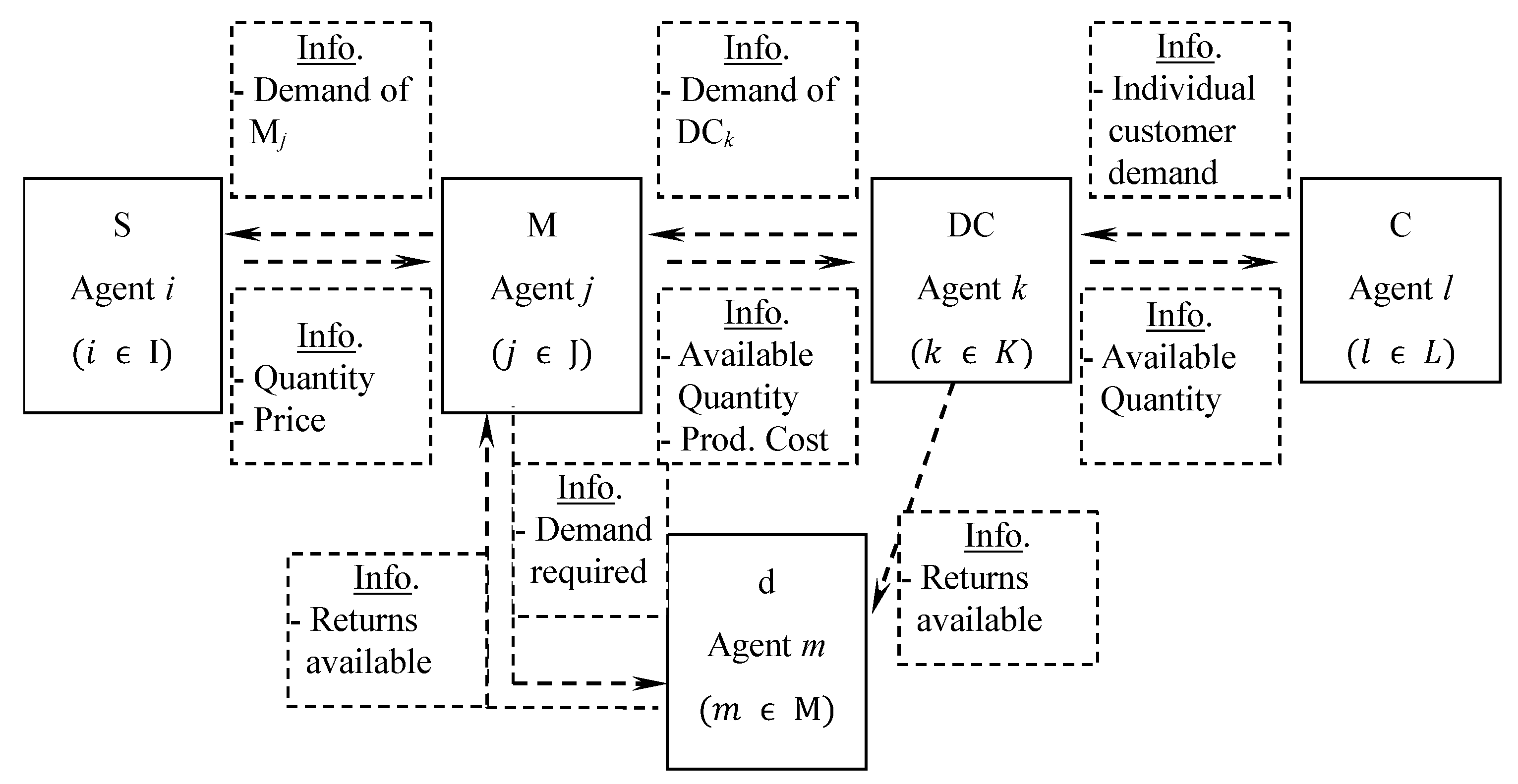
The CLSC is modeled by using the multi-agent based approach shown in Figure 2. It consists of 5 types of agents: Supplier Agents (Si), Manufacturing Agents (Mj), Distribution Center Agents (DCk), Customer Agents (Cl) and Dismantler Agent (dm). The operation of the system is driven by the demands coming from customers, which are supplied by the DCs. Meanwhile, DCs are supplied by the manufacturers, who will then determine the production quantity and further initiates demand to suppliers. In this CLSC multi-agent model, this demand information will only be shared between two layers, such as the agents in the layer of S with M, M with DC, DC with C, DC with d and d with M in order to simplify the problem complexity. Accordingly, we propose a novel two-stage priority based Genetic Algorithm (GA) for this multi-agent modeling approach. The algorithm deals with 2 main issues, (i) pairing up each pair of agents between every layer and (ii) determining the actual quantity.

4. A Two-Stage Priority-Based Genetic Algorithm Encoding with Multi-Agent

In this proposed CLSC problem, the objective is to identify an applicable delivery route and corresponding product flow volume to obtain the minimum cost of transportation and facility operation. Here two problems have to be solved simultaneously; one is to decide the handling quantity of each active facility and the other is to decide the transportation route among the whole network. Additionally, these two problems are under a six-level CLSC which makes the problem more complicated.

By using the single-stage encoding GA, these two problems have to be expressed in a single chromosome, which means the chromosome must be able to convey the information on the route and volume and also the active state of the facilities. These vast amounts of information will make the genetic operation too complicated to handle because of too many possible combinations. In addition, this chromosome structure will obviously increase the calculation time. Since all the information is considered at the same time, the search is easy to get lost in the local optimum.

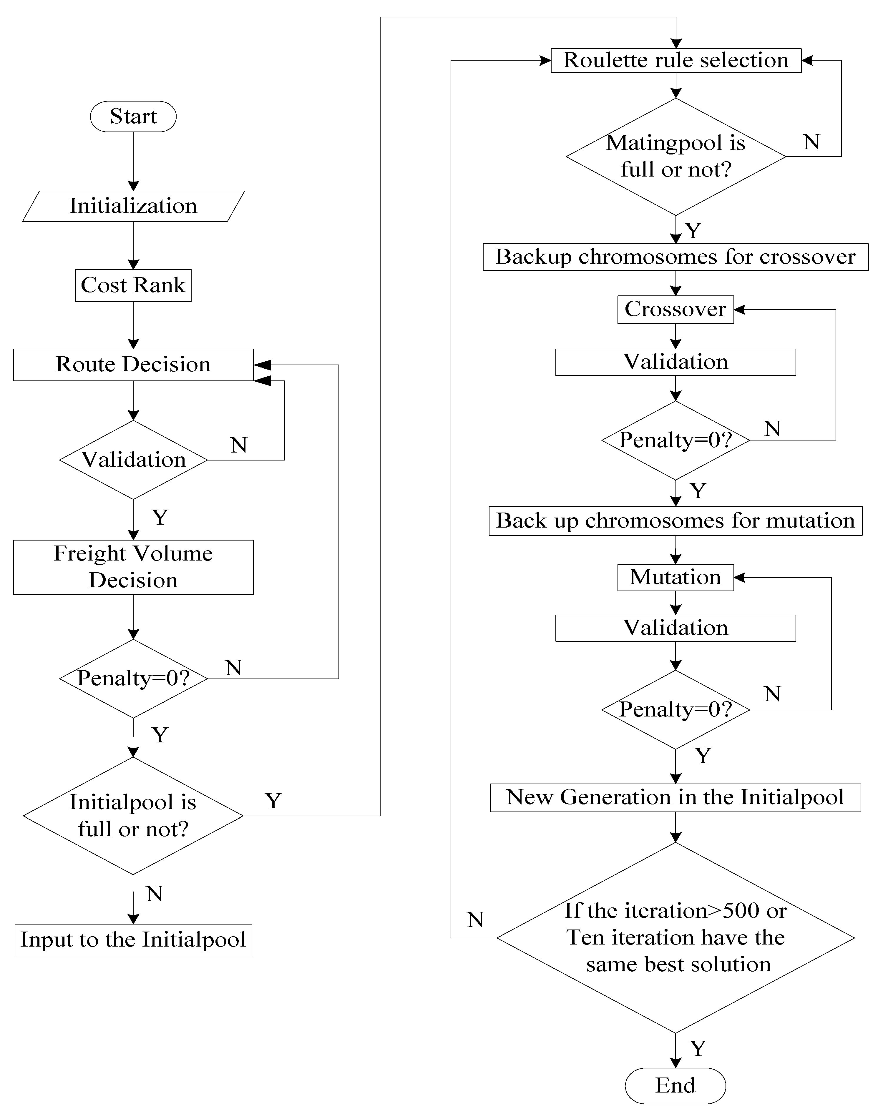
To deal with the problem, a two-stage priority-based GA with multi-agent approach is established. The proposed approach divides the encoding process into two stages, which express the above mentioned two problems in the CLSC network respectively. Figure 3 shows the flow diagram of this developed approach.

From Figure 3, it can be observed that this GA approach has two stages in the encoding process including Stage 1 “Route Decision”, Stage 2 “Freight Volume Decision”. Route Decision stage is used to decide the delivery route in the proposed CLSC network. It also applied to determine the pairing of agents. Freight Volume Decision stage is applied to determine the freight volume for each selected route according to the results of stage 1. These two stages are carefully described in Section 4.1 and Section 4.2 respectively. The “Cost Rank” process before “Route Decision” is the preparation of the priority-based “Freight Volume Decision” which is explained in Section 4.2. The right part of Figure 3 describes the genetic operations. Section 4.3 gives details.

4.1. Stage 1—Route Decision

The first stage of encoding is to decide the applicable delivery route. In the first stage, the chromosome generated consist of binary genes, which only represent the information of delivery route. Since the chromosomes, in stage 1 only deliver the information of transportation route except for the quantity of product flow, it makes the genetic operations, especially the validation, much more concise than the traditional GA.

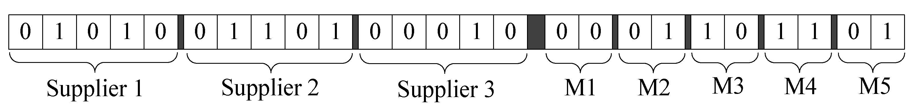
The chromosome possesses six sections corresponding to the six levels of the CLSC model. In each section, the amount of genes is equal to the product of the amount of suppliers and the amount of demanders. In general, the number of genes in a chromosome, is expressed by $I\times J+J\times K+K\times L+L\times K+K\times M+M\times J$, where I, J, K, L and M are the number of suppliers, manufacturers, distribution centers, customers and dismantlers respectively.

To explain the proposed algorithm clearly, a numerical example is provided. In this example, I = 3, J = 5, K = 2 which means that three suppliers provide materials to five manufacturers and these five manufacturers provide finished products to two DCs. The chromosome at this stage in the example is shown in Figure 4 and the corresponding delivery route is shown in Figure 5a.

In Figure 4, each gene holds a binary number, where 1 indicates the delivery route is adopted and 0 indicates it is not. Figure 4 shows that there has 15 genes for the first section of the chromosome. The first five genes illustrates the condition where supplier 1 provises materials to manufacturers 2 and 4 but does not provide materials to manufacturers 1, 3 and 5. The second five genes and the third five genes illustrate the related information of supplier 2 and supplier 3, respectively. Figure 4 also shows that there has 10 genes for the second section of the chromosome. The first two genes describe the condition where manufacturer 1 does not provide finished products to both two DCs. Similarly, the following four groups of genes describe the related information of the corresponding manufacturers. Figure 5a illustrates the delivery route. The numbers in parentheses means the unit transportation cost of each delivery route and the numbers in circles means the capacity of each partners.

4.2. Stage 2—Freight Volume Decision

After the pairing, a delivery route is determined. Now, we have to decide the quantity for each agent needs to obtain. The second stage is to determine the freight volume of materials or products, and the chromosome encoded in the second stage is shown in Figure 6.

Figure 6 show that the structure of the chromosome in stage 2 is the same as that in stage 1, but the composition of each gene is indeed different. The first five genes illustrates the condition where supplier 1 will deliver 50 units of raw materials to manufacture 2 and supplier 4, but will not delivery any raw materials to manufacturers 1, 3 and 5. The second five genes and the third five genes illustrate the related information of supplier 2 and supplier 3, respectively. The last two genes for the second section of the chromosome describe the condition where manufacturer 5 will deliver 200 units of products to distribution center 2 but will not deliver any products to distribution center 1. The network including delivery route and freight volume are shown in Figure 5b.

4.2.1. Process Outline

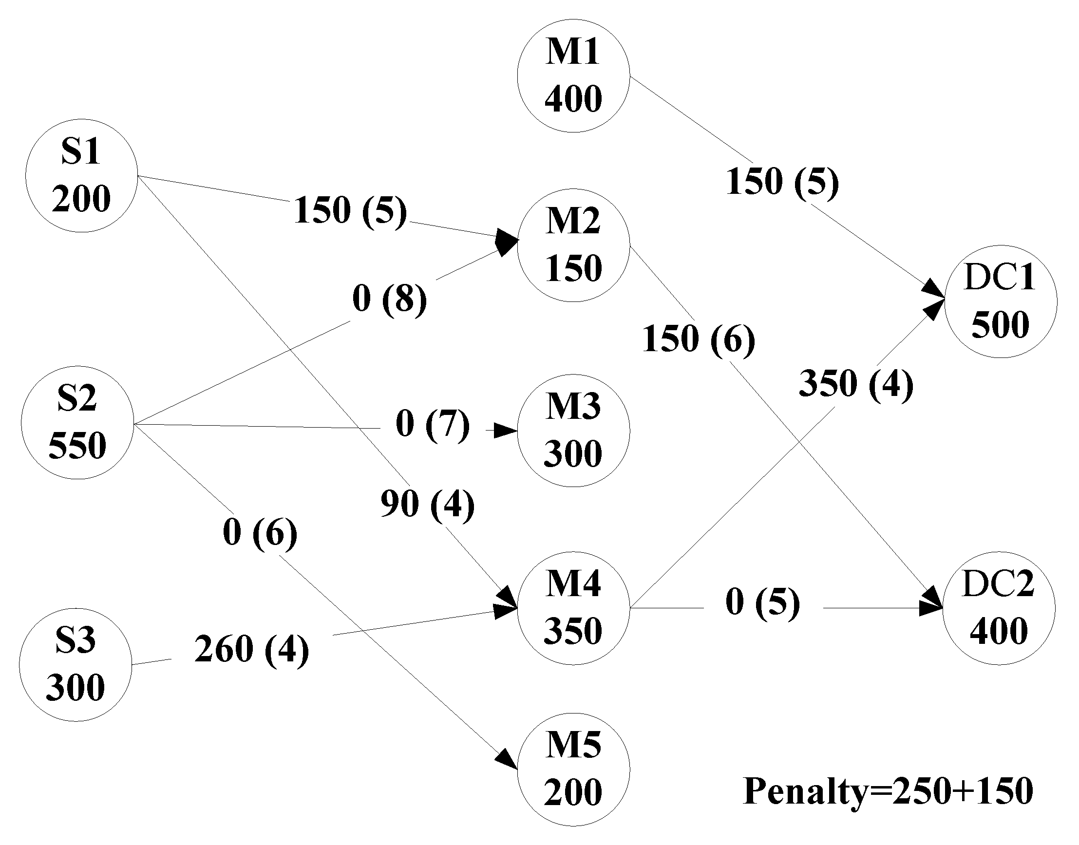
It is turned out that six steps are needed to determine the freight volume during freight volume decision process. To explain the freight volume decision process in detail, the numerical example in Section 4.1 is used. In this three stage supply chain example, the step details are illustrated in Figure 5 and described as below. The numbers in parentheses indicate the unit transportation cost of the delivery route. The numbers in the circles indicate the request of the distribution centers and the capacity of suppliers and manufacturers.

Step I:

Determine the start level in the supply chain network. In this case, the terminal demand is at the distribution centers, hence the freight volume decision process begins at the level from manufacturer to distribution center.

Step II:

Detect the top priority delivery route with the lowest unit shipping cost in the current level. According to the result of “Cost Rank,” the lowest unit shipping cost within current level is 3, which is from manufacturer 3 to distribution center 1. The detail of “Cost Rank” will be explained in Section 4.2.2.

Step III:

Check if there are other delivery routes with the same unit shipping cost and also the same demand as the one found in Step 2. In other words, check if the top priority delivery route is multiple or not. If the result is yes, count out the number, mark as N and go to Step 4a, if not, go to Step 4b. Step 4a and Step 4b are parallel. In this example, this unit shipping cost 3 is unique at this level, so go to Step 4b.

Step IVa:

Devide the demand into N parts randomly and assigned them to the N delivery routes with the top priority.

Step IVb:

Assign the smaller one to the transport flow through the comparison between the supply capability and the demand. Due to the supply capability of manufacturer 3 is 300 units and the demand of distribution center 1 is 500 units, the freight volume between them is 300 units.

Step V:

Renew the corresponding supply capability and demand. The remaining supply capability of manufacturer 3 is 300 − 300 = 0 and the renewed demand of distribution center 1 is 500 − 300 = 200.

Step VI:

Move to the next delivery route on the basis of the result of “Cost Rank” and then repeat Step 2 to Step 6. When the entire level is completed, return to the next level. In this example, the delivery route between manufacturer 4 and distribution center 1 is found out according to “Cost Rank” as the next operand.

Specifically, when the unit transportation cost of several different suppliers delivering to the same demander is the same, the delivery flow will be randomly produced. In this case, since the unit transportation cost of both manufacturer 2 and manufacturer 5 to distribution center 2 are 6, the corresponding flows are randomly generated to be 50 and 200 respectively.

4.2.2. Order Bidding Strategy: Cost Priority Rule

At this stage, every agent will now be allocated with a certain quantity on hand. This quantity has to be supplied by its immediate up stream suppliers. To determine the winning supplier, we propose a Cost Priority Rule. In this case, each delivery route produces its own unit transportation cost. The route with low transportation costs will have priority for use, which is called cost priority rule.

This cost priority rule is much proper in this problem than other rules such as demand priority and equal distribution. With this rule, the freight volume decision process can reach the edge value of the transportation cost in the whole CLSC under the pre-decided delivery route. Hence it can enhance the efficiency of the genetic search and increase the calculation speed. The flow allocation has to begin at the last stage of the proposed supply chain due to the imperative satisfaction of demand. It means the flow allocation begins from the level of distribution centers delivery to customers in the forward chain and then, move to the level of the manufacturers’ delivery to the distribution centers. After that, rather than moving to the suppliers, it jumps to the reverse chain, which starts at the level of customers’ recovery to the distribution centers and then, to dismantlers and manufacturers. The flow allocation of suppliers delivering to manufacturers is implemented as the end procedure, because the manufacturing demand depends on both the demand of the distribution centers in the forward chain and the supply quantity of the dismantlers in the reverse chain.

4.3. Genetic Operations

Genetic operations are indispensable parts in genetic algorithms. In the proposed problem, one-point crossover and one-point mutation is implemented to avoid dramatic changes in genetic structure due to the particular chromosome properties, which will prevent random genetic searches additionally.

4.3.1. Fitness Function

The fitness function is to calculate the fitness value of each chromosome which represents the viability of the chromosomes. In the proposed model, the fitness is assigned as reciprocal of the total cost. Lower total cost indicates stronger chromosome viability.

$$Fitness=\frac{1}{Total Cost}$$

$$Total cost=Fix cost+Transportation cost$$

$$Fix cost={\displaystyle \sum _j{f}_j{\alpha }_j}+{\displaystyle \sum _k{g}_k{\beta }_k}+{\displaystyle \sum _m{h}_m{\delta }_m}+\phi {\displaystyle \sum _m\lfloor p{l}_m{\displaystyle \sum _k{o}_{km}}\rfloor }$$

$$Transportation cost={\displaystyle \sum _{\mathrm{i}}{\displaystyle \sum _j{s}_{ij}{x}_{ij}}}+{\displaystyle \sum _j{\displaystyle \sum _k{t}_{jk}{y}_{jk}}}+{\displaystyle \sum _k{\displaystyle \sum _l{u}_{kl}{z}_{kl}}}+{\displaystyle \sum _k{\displaystyle \sum _m{v}_{km}{o}_{km}}}+{\displaystyle \sum _m{\displaystyle \sum _j{w}_{mj}R{d}_{mj}}}+{\displaystyle \sum _l{\displaystyle \sum _{k}R{u}_{lk}R{z}_{lk}}}.$$

4.3.2. Selector Operator

In this proposed GA, after generating the initial pool randomly, generation of the mating pool is based on the roulette wheel selection. In this roulette wheel selection, the fitness function is used to decide the selected probability for each chromosome. The roulette wheel function is

$$p_i=\frac{f_i}{{\displaystyle \sum _j{f}_j}},$$

here $p_i$ means the selected probability for chromosome i, $f_i$ means the fitness of chromosome i.

4.3.3. Crossover

In this algorithm, one-point crossover is applied. The characteristic of one-point crossover is that genes within parent chromosome will not change greatly, therefore, after several evolution, weak genes will be identified easily [31]. In this CLSC problem, the chromosomes contains several sections, each section represents one stage in the supply chain network. Since weak genes cause weak section, weak genes identification is crucial. This crossover process contains three steps as shown in Figure 7.

Step 1:

Pick up two parents from the mating pool randomly.

Step 2:

Randomly generate the cut point.

Step 3:

Generate two offspring according to the cut point.

4.3.4. Mutation

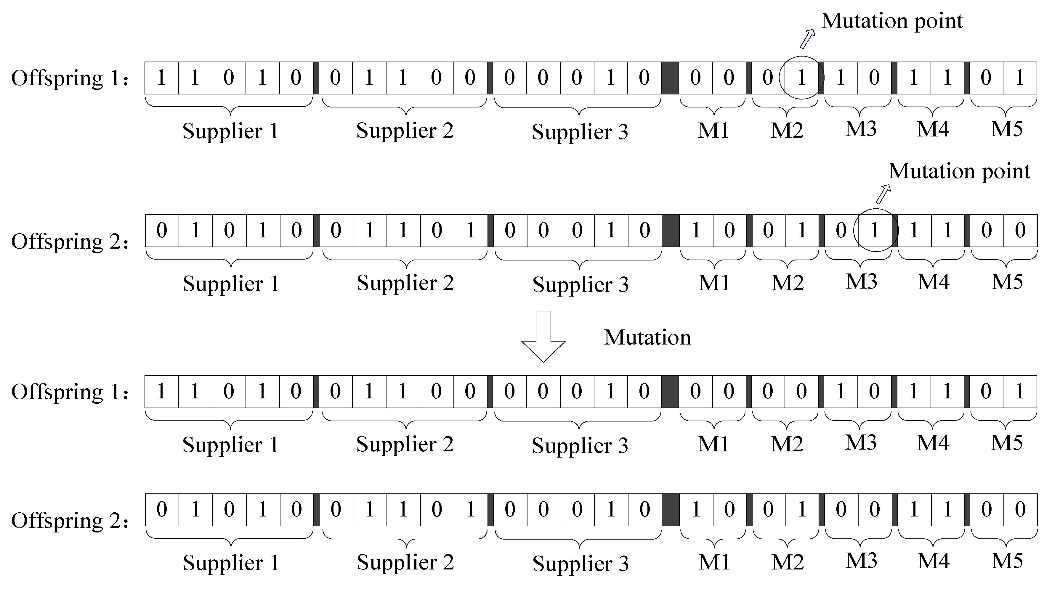
Due to the special feature of this two-stage encoding, the search of the proposed method is more easily trapped in a local optimum. Mutation process can prevent this situation. Therefore, one-point mutation is implemented, in which the mutation rate is set to 1. The process of mutation contains three steps as shown in Figure 8.

Step 1:

Pick up one chromosome from the mating pool.

Step 2:

Randomly generate a mutation point and read the number of this gene as A.

Step 3:

Calculate the result of 1 minus A and load this result to the gene of the selected mutation point.

4.3.5. Validation

In order to guarantee the feasibility after crossover and mutation, validation is implemented. Due to the characteristics of two-stage encoding, the validation contains two parts.

Part 1: Check Capacity Requirements

There are several situations for offspring invalidation after crossover and mutation. In Part 1, the procedure checks on the binary chromosome, which is the chromosome before the “freight volume decision.” If one of the situations in

Table 1. Capacity requirements.

Validation Requirements
1. Active distribution centers must have enough capacity to satisfy customers demand totally.
2. Active manufacturers must have enough capacity to satisfy customers demand totally.
3. Since each customer must recovery at least one return product to distribution centers, the customer genes are forbidden to be zero simultaneously.
4. Customer must have at least one corresponding distribution center due to the satisfaction need of customers.

occurs, rollback of crossover and mutation processes will be implemented.

Take Figure 7 for example, the active manufacturers in offspring 1 is M3, M4 and M5. In this case, the total capacity can’t satisfy the total customer demand, which causes invalidation to rollback the whole crossover process. The selected parents chromosome will be assigned as the offspring after crossover.

Part 2: Check Penalty

If the offspring get through the capacity check in Part 1, the penalty check in Part 2 will be implemented. In Part 2, this validation procedure acts on the integer chromosome, which is the chromosome after the “freight volume decision.” In this step, the penalty for the transformed chromosome is examined. If the penalty is not equal to zero as before, the procedure will undo the whole process of respective crossover and mutation.

In Figure 8, offspring 2 after mutation shows the invalidation of the penalty in Part 2. To show the detail and explain the calculation process of the penalty, the network of offspring 2 is drawn in Figure 9.

4.3.6. Stopping Condition

The proposed approach will improve the initial pool iteratively until one of the stopping conditions below is met: a preset maximum number of generations is reached or a feasible solution is generated in twenty successive generations.

5. Computational Experiments

In this section, three computational experiments are implemented to demonstrate the efficiency and stability of the proposed approach. For the convenience of comparison, the same dataset as Wang and Hsu’s paper [17] is used for Experiment 1. In this referenced paper, a revised spanning-tree based GA was proposed to optimize the CLSC model. The great difference between the fixed costs of the entities in Experiment 1 shows that it is an extreme case in this computational experiment. Hence, Experiment 2 and Experiment 3 are needed to illustrate more usual cases. Based on existing literature, such as Atabaki et al. [22] and Min et al. [28], we make some changes and improvements in the following experiments. Their exist similar values within the capacity and fixed cost of distribution centers in Experiment 2, which make the optimal search become difficult. In Experiment 3, the fixed cost and the corresponding capacity within same level entities are set to be even more closer to make the optimal search even more difficult. All of the three experiments include five sub-problems with a scale from basic to large.

Table 2. Scale of computational experiments.

	Supplier	Manufacture	DC	Customer	Dismantler
Basic Scale	3	5	3	4	2
Second Scale	6	10	6	8	4
Third Scale	12	20	12	16	8
Fourth Scale	24	40	24	32	16
Fifth Scale	48	80	48	64	32

shows the five scales.

5.1. Experiment 1

In this experiment, the dataset in Wang and Hsu’s paper [17] has been used. With the same input data, the comparison between the single-stage encoding spanning tree based GA and the proposed GA is convincing.

After computing the proposed two stage priority and multi-agent based GA, the result of the basic scale problem turns to be uniform with the referenced paper. In other words, with the uniform of the total costs, their exist slightly differents in the flow volume between each level. This result indicates the acquirement of another optimal solution for this NP-hard problem.

To further test the proposed approach, four larger scale problems have been computed. The dataset is also the same as the original paper.

Table 3. Comparison of the proposed approach and the spanning tree based GA.

30 Times EACH Problems	Scale	Numerical Examples
		1	2	3	4	5
Revised ST-GA (population size = 100) in original paper	Min-cost (US$)	29,848	58,368	115,866	235,309	469,089
	Ave-cost (US$)	29,966	58,999	117,524	237,820	470,310
	Ave-time (s)	2.04	6.35	22.49	72.74	356.28
Two stage priority based GA (population size = 100)	Min-cost (US$)	29,848	58,325	115,246	232,983	463,117
	Ave-cost (US$)	29,931	58,867	116,865	234478	464,445
	Ave-time (s)	0.09	1.21	9.25	40.25	230.80
Results comparison	Absolute difference	0	43	620	2326	5972
	Percentage difference	0	0.07%	0.54%	0.99%	1.27%
Average time comparison	Absolute difference	1.95	5.14	13.24	32.49	125.48
	Percentage difference	95.6%	80.9%	58.9%	44.7%	35.2%

shows the comparison between the proposed approach and the revised spanning tree based GA (Revised ST-GA) in Wang and Hsu’s paper [17].

Table 4. Comparison between the proposed approach and Lingo.

30 Times Each Problems	Scale	Numerical Examples
		1	2	3	4	5
Lingo 11.0	Optimal (US$)	29,848	58,306	114,805	228,092	455,041
	Time (s)	1	12	>1000	>2700	>9000
Two stage priority based GA (population size = 100)	Min-cost (US$)	29,848	58,325	115,246	232,983	463,117
	Absolute difference	0	−19	−447	−4891	−8076
	Percentage difference	0	−0.03%	−0.38%	−2.14%	−1.77%
	Average-cost (US$)	29,931	58,867	116,865	234,478	464,445
	Average-time (s)	0.09	1.21	9.25	40.25	230.80
	Percentage of time	9%	10.1%	<0.93%	<1.49%	<2.56%

shows the comparison between the proposed GA and Lingo. The results of Lingo and the provided GA are worked out using a HP PC with Intel(R) Core(TM) i7-2600 CPU @ 3.4 GHz, 8.0 G RAM. The result of the referenced paper was obtained using a PC with Intel^® Pentium^® M processor 1.86 GHz, 1.0 G RAM.

In Table 3, the results of revised ST-GA are from the original paper. Suite reference again, from the optimal value comparison and the average time comparison, it is obvious that the proposed approach can produce higher quality results within a shorter computing time. Take Scale 2 for example, in the optimal value comparison, the percentage difference is 0.07%, which means the result of the proposed approach is 0.07% better than the spanning tree GA. Furthermore, in the average time comparison, the percentage difference is 80.9%, which means the running time of the proposed approach is 80.9% faster than the spanning tree GA. When the scale of problem increases, the accuracy of the proposed approach is improving and the running time is always shorter. In Scale 3, the result of the proposed approach is 0.54% better than the spanning tree GA and the average running time is 58.9% better. In Scale 4, the result of the proposed approach increases to 0.99% better with 44.7% of the running time, which is twice as fast as the speed of the spanning tree GA. Furthermore, in Scale 5, when the number of variables is almost 19,000, the quality result is 1.27% better than the spanning tree GA with about one third of the running time 35.2%.

Table 4 indicates the comparison results of Lingo 11.0 and the proposed approach with five scales. The “absolute difference” row shows the value of the Lingo values minus the results of the proposed approach. The minus sign means disparity. For instance, in Scale 2, the absolute difference value is −19, the value of percentage difference is −0.03%, which indicates the disadvantageous of the proposed approach is 0.03% compared to Lingo. However, the average running time of the proposed approach is 1.21 s, which is only 10.1% of the time from Lingo. When the scale of the problem grows larger, the speed advantage of proposed approach is more obvious. In Scale 3, the disadvantageous of the proposed approach is 0.38% compared to Lingo, but the running time is less than 0.93% compared with Lingo. In Scale 4, the disadvantageous of the proposed approach is 2.14% compared to Lingo, but the time of running is less than 1.49%. In Scale 5, while the performance of the proposed approach is 1.77% behind Lingo, the running time is better than Lingo by almost 40 times. Furthermore, if the scale of problems keeps growing, Lingo cannot even give out an optimal result within an acceptable time. However, the proposed approach can solve it effectively.

In this basic scale model, the landfilling rate is set to 0.1 currently. To test the robustness of the results and study the influence of the landfilling rate on the total cost, we provide a sensitivity analysis. Since it is an integer programming, which is discrete, we illustrate an arithmetic sequence in the range of landfilling rate which is from 0 to 1. Where 0 means no landfilling and 1 means landfilling all without recycling.

Table 5. The relationship between landfilling rate and total cost.

Variable	Value
Landfilling Rate	0	0.05	0.1	0.15	0.2	0.25	0.3
Total cost	29,743	29,849	29,848	29,961	29,953	30,019	30,058
Landfilling rate	0.35	0.4	0.45	0.5	0.55	0.6	0.65
Total cost	30,185	30,163	30,297	30,268	30,409	30,373	30,521
Landfilling rate	0.7	0.75	0.8	0.85	0.9	0.95	1
Total cost	30,478	30,551	30,583	30,754	30,688	30,857	30,793

shows the calculation results of the landfilling rate and the corresponding total cost. Figure 10 shows the line graph of the relationship between landfilling rate and the total cost. From Table 5 and Figure 10, it can be seen that the total cost increases slightly with the increase of the landfilling rate and remains basically constant, which indicates that the model has a good robustness.

5.2. Experiment 2

The results of Experiment 1 show that, manufacturer 1, manufacturer 4 and distribution center 3 are not used due to their high fixed cost and low capacity. To make the model more complex, manufactures fixed cost and distribution centers fixed cost are reset. To release more active entities, the unit shipping costs are reset too. After the data changing, the parameters within distribution centers become similar, which tight the optimal solution to make the optimal search more difficult.

Table 6. Capacity, fixed cost (US$) and demand in Experiment 2.

Supplier Capacity	Manufacture		DC		Customer	Dismantler
	Capacity	Fixed Cost	Capacity	Fixed Cost	Demand	Capacity	Fixed Cost
500	400	1100	870	1000	500	540	900
650	550	900	890	900	300	380	800
390	490	2100	600	800	400
	300	800			300
	500	900

shows the capacity and fixed cost.

Table 7. Unit shipping cost for each stage (US$) in Experiment 2.

Manufacture	DC			Customer	DC
	1	2	3		1	2	3
1	5	8	5	1	3	7	4
2	8	6	8	2	8	5	5
3	5	7	4	3	4	4	4
4	3	5	3	4	3	3	5
5	5	6	6

indicates the unit shipping costs.

Since the dataset is different to that in the original paper [17], the comparison is only between the proposed approach and Lingo. For simplicity, only the dataset of the basic scale is shown. The other four scales are doubled and redoubled to the basic scale, which was the same data building method as that in the original paper [17]. The optimal solution is shown in

Table 8. The optimal solution of Experiment 2.

Objective Value						29,099
$x_{ij}$	$x_{13}=100$	$x_{15}=365$	$x_{22}=510$	$x_{33}=390$
$y_{jk}$	$y_{22}=510$	$y_{33}=490$	$y_{51}=500$
$z_{kl}$	$z_{12}=290$	$z_{14}=210$	$z_{21}=500$	$z_{22}=10$	$z_{33}=400$	$z_{34}=90$
$o_{km}$	$o_{12}=87$	$o_{22}=3$	$o_{32}=60$
$R{d}_{mj}$	$R{d}_{25}=135$
$R{z}_{lk}$	$R{z}_{11}=50$	$R{z}_{22}=3$	$R{z}_{23}=27$	$R{z}_{31}=7$	$R{z}_{33}=33$	$R{z}_{41}=30$
${\alpha }_j$	${\alpha }_2=1$	${\alpha }_3=1$	${\alpha }_5=1$
${\beta }_k$	${\beta }_1=1$	${\beta }_2=1$	${\beta }_3=1$
${\delta }_m$	${\delta }_2=1$

.

Table 9. Comparison with Lingo in Experiment 2.

30 Times Each Problems	Scale	Numerical Examples
		1	2	3	4	5
Lingo 11.0	Optimal (US$)	29,099	55,817	110,137	218,677	436,697
	Time (s)	1	4	>1000	>2700	>9000
Two stage priority based GA (population size = 100)	Min-cost (US$)	29,099	55,936	111,172	226,053	447,644
	Absolute difference	0	−119	−1035	−7376	−10,947
	Percentage difference	0	−0.21%	−0.94%	−3.37%	−2.50%
	Average cost (US$)	29,173	56,385	112,258	228,165	449,377
	Average time (s)	0.15	1.12	9.37	73.33	258.40
	Percentage of time	15%	28%	<0.94%	<2.72%	<2.87%

is the comparison with Lingo.

Since Lingo is an exact algorithm and GA is a heuristic algorithm, it is usual that Lingo can get better results when the calculation scale is relatively small. But when the calculation scale gets large, Lingo may cannot get an acceptable result within an acceptable period of time. That’s where heuristic algorithm works.

From Table 9, it can be seen that although the quality of results is reduced, the calculation speed is far faster than Lingo. In Scale 1, the proposed approach can find the same optimal solution as Lingo within a shorter time, which is only 15% of the Lingo running time. In Scale 2, the disadvantageous is 0.21% compare to Lingo, but the time of running is only 28%. When the scale grows to Scale 3, the result is 0.94% poorer than Lingo but the running time shorts to less than 0.94% of it. In Scale 4, the disadvantageous is 3.37% compare to Lingo, however the running time shortens to 2.72%. In Scale 5, the disadvantageous becomes 2.5% compare to Lingo, while the time of running is less than 2.87%. It is observed from the “Percentage difference” row that all of the disadvantageous are below 3.5%, however, the running time in the “Percentage of time” row are 100 times faster than Lingo.

5.3. Experiment 3

In order to further tight the optimal solution of the whole network to add difficulties in the searching, the parameters are further modified. From the optimal solution of the basic scale in Experiment 3 shown in

Table 10. The optimal solution of Experiment 3.

Objective Value						26,771
$x_{ij}$	$x_{11}=400$	$x_{22}=200$	$x_{25}=450$	$x_{32}=150$	$x_{32}=150$	$x_{34}=165$
$y_{jk}$	$y_{13}=400$	$y_{22}=350$	$y_{41}=300$	$y_{51}=300$	$y_{52}=150$
$z_{kl}$	$z_{12}=300$	$z_{14}=300$	$z_{21}=500$	$z_{33}=400$
$o_{km}$	$o_{11}=61$	$o_{21}=89$
$R{d}_{mj}$	$R{d}_{14}=135$
$R{z}_{lk}$	$R{z}_{11}=50$	$R{z}_{22}=30$	$R{z}_{32}=40$	$R{z}_{41}=11$	$R{z}_{42}=19$
${\alpha }_j$	${\alpha }_1=1$	${\alpha }_2=1$	${\alpha }_4=1$	${\alpha }_5=1$
${\beta }_k$	${\beta }_1=1$	${\beta }_2=1$	${\beta }_3=1$
${\delta }_m$	${\delta }_1=1$

, it can be seen that four manufacturers and three distribution centers are being used.

For clarity, only the changed part of the unit shipping cost is shown, the other part is the same as that in Experiment 2.

Table 11. Capacity, fixed cost (US$) and demand in Experiment 3.

Supplier Capacity	Manufacture		DC		Customer Demand	Dismantler
	Capacity	Fixed Cost	Capacity	Fixed Cost		Capacity	Fixed Cost
500	450	400	870	1000	500	540	900
650	350	740	890	900	300	380	800
390	400	1900	600	800	400
	300	600			300
	600	600

shows the capacity and fixed cost.

Table 12. Unit shipping cost for each stage (US$) in Experiment 3.

Supplier	Manufacture					Manufacture	DC
	1	2	3	4	5		1	2	3
1	5	6	4	7	5	1	6	8	5
2	6	5	6	6	4	2	4	3	5
3	7	6	3	5	6	3	5	7	4
						4	3	5	3
						5	5	6	6

shows the unit shipping cost for each stage. The optimal solution is shown in Table 10.

Table 13. Comparison with Lingo in Experiment 3.

30 Times Each Problems	Scale	Numerical Examples
		1	2	3	4	5
Lingo 11.0	Optimal (US$)	26,771	51,667	101,947	202,097	403,570
	Time (s)	1	8	>1000	>2700	>9000
Two stage priority based GA (population size = 100)	Min-cost (US$)	26,771	51,892	103,714	211,602	419,135
	Absolute difference	0	−225	−1767	−9505	−15565
	Percentage difference	0	−0.44%	−1.73%	−4.70%	−3.86%
	Average cost (US$)	26,772	52,528	104,793	213,463	421,102
	Average time (s)	0.12	1.25	9.21	49.52	267.34
	Percentage of time	12%	15.60%	<0.90%	<1.83%	<2.97%

is the comparison with Lingo.

Table 13 shows the results and comparison with Lingo. In Scale 1, the proposed approach can obtain the optimal solution within just 12% of the running time of Lingo. In Scale 2, the disparity is 0.44% to Lingo but the running time is 15.6%. When the problem scale grows to Scale 3, the result is a 1.73% disadvantage to that of Lingo but the time is less than 0.9%. In Scale 4, the disadvantageous is 4.7% compare to Lingo, but the running time is less than 1.83%. In Scale 5, the disparity is 3.86% to Lingo, however, the running time is less than 2.97%. In Experiment 3, the optimal search becomes more difficult, while the error rate is still below 5%, which can be checked from the “Percentage difference” row. The “Percentage of time” row indicates the obvious advantage of the running time performance. From the results of Experiment 3, it can be further demonstrated that when the scale of the problem grows, the proposed approach can still give a near optimal solution with a fast calculation time.

6. Conclusions and Suggestions of Future Work

Due to growing environmental issues nowadays, product recycling problems within closed-loop supply chain draws more attention. To solve these problems, many CLSC models have been established in this research area. A six-level CLSC model studied in this paper can be transformed into an integer linear programming model. The small-scale calculation of this model can be solved by using LINGO. However, LINGO cannot solve the large-scale model in an acceptable time. This is due to that the complexity of the model will increase as the scale increases. A spanning-tree based GA is proposed by Wang and Hsu [17] in 2010 so as to solve the problem. However, the single-stage encoding method cannot reach a fully exploit of the search ability of GA. In this study, a new two-stage priority-based GA encoding with multi-agent has been established to improve the solution of this kind of CLSC model. It helps to the research of implementing GA more efficiently on the CLSC problem.

Three computational experiments have been implemented. Experiment 1 has the same dataset as Wang and Hsu’s experiment and the results show that the proposed algorithm can reliably obtain higher quality solutions in a shorter computation time. Since Experiment 1 is an extreme case with several entities idling, Experiment 2 and Experiment 3 are implemented to demonstrate the performance of the proposed approach in usual cases. In Experiment 2, all of the distribution centers are close in fixed cost and capacity which makes the optimal search more difficult. The results of Experiment 2 demonstrate that the proposed approach can get high quality results within shorter running times. Experiment 3 reset the parameters within the whole network to further tight the optimal solution, so as to make the optimal search even more difficult. The results of Experiment 3 show that the proposed approach still can provide a competent solution. Throughout these three computational experiments, the efficiency and stability of the proposed algorithm is proven. In the real case, the product flow in the CLSC network contains different kinds of products. In this sence, multi-product can be considered in future research.

References

- Krikke, H.; Bloemhof-Ruwaard, J.; Van Wassenhove, L.N. Concurrent product and closed-loop supply chain design with an application to refrigerators. Int. J. Prod. Res. 2003, 41, 3689–3719. [Google Scholar] [CrossRef]
- Guide, V.D.R.; Van Wassenhove, L.N. Closed-loop supply chains: An introduction to the feature issue (part 1). Prod. Oper. Manag. 2006, 15, 345–350. [Google Scholar] [CrossRef]
- Guide, V.D.R.; Van Wassenhove, L.N. The Evolution of Closed-Loop Supply Chain Research. Oper. Res. 2009, 57, 10–18. [Google Scholar] [CrossRef]
- Gen, M.; Altiparmak, F.; Lin, L. A genetic algorithm for two-stage transportation problem using priority-based encoding. Or Spectr. 2006, 28, 337–354. [Google Scholar] [CrossRef]
- Fleischmann, M.; BloemhofRuwaard, J.M.; Dekker, R.; van der Laan, E.; van Nunen, J.; Van Wassenhove, L.N. Quantitative models for reverse logistics: A review. Eur. J. Oper. Res. 1997, 103, 1–17. [Google Scholar] [CrossRef] [Green Version]
- Wells, P.; Seitz, M. Business models and closed-loop supply chains: A typology. Supply Chain. Manag. 2005, 10, 249–251. [Google Scholar] [CrossRef]
- Abu Bakar, M.S.; Rahimifard, S. Computer-aided recycling process planning for end-of-life electrical and electronic equipment. Proc. Inst. Mech. Eng. Part B J. Eng. Manuf. 2007, 221, 1369–1374. [Google Scholar] [CrossRef] [Green Version]
- Olugu, E.U.; Wong, K.Y. An expert fuzzy rule-based system for closed-loop supply chain performance assessment in the automotive industry. Expert Syst. Appl. 2012, 39, 375–384. [Google Scholar] [CrossRef]
- Yan, R.; Yan, B. Location model for a remanufacturing reverse logistics network based on adaptive genetic algorithm. Simul. -Trans. Soc. Model. Simul. Int. 2019, 95, 1069–1084. [Google Scholar] [CrossRef]
- Sheu, J.B.; Chou, Y.H.; Hu, C.C. An integrated logistics operational model for green-supply chain management. Transp. Res. Part E -Log. 2005, 41, 287–313. [Google Scholar] [CrossRef]
- Ozceylan, E.; Paksoy, T. A mixed integer programming model for a closed-loop supply-chain network. Int. J. Prod. Res. 2013, 51, 718–734. [Google Scholar] [CrossRef]
- Hitchcock, F.L. The distribution of a product from several sources to numerous localities. J. Math. Phys. 1941, 20, 224–230. [Google Scholar] [CrossRef]
- Aikens, C.H. Facility Location Models for Distribution Planning. Eur. J. Oper. Res. 1985, 22, 263–279. [Google Scholar] [CrossRef]
- Ko, H.J.; Evans, G.W. A genetic algorithm-based heuristic for the dynamic integrated forward/reverse logistics network for 3PLs. Comput. Oper. Res. 2007, 34, 346–366. [Google Scholar] [CrossRef]
- Akcali, E.; Cetinkaya, S. Quantitative models for inventory and production planning in closed-loop supply chains. Int. J. Prod. Res. 2011, 49, 2373–2407. [Google Scholar] [CrossRef]
- Chen, Y.T.; Chan, F.T.S.; Chung, S.H. A two-stage priority based genetic algorithm for closed-loop supply chain network. In Proceedings of the 2nd International Congress on Engineering and Information (ICEAI 2013), Bangkok, Thailand, 26–28 January 2013; pp. 209–215. [Google Scholar]
- Wang, H.F.; Hsu, H.W. A closed-loop logistic model with a spanning-tree based genetic algorithm. Comput. Oper. Res. 2010, 37, 376–389. [Google Scholar] [CrossRef]
- Barros, A.I.; Dekker, R.; Scholten, V. A two-level network for recycling sand: A case study. Eur. J. Oper. Res. 1998, 110, 199–214. [Google Scholar] [CrossRef]
- Paksoy, T.; Bektas, T.; Ozceylan, E. Operational and environmental performance measures in a multi-product closed-loop supply chain. Transp. Res. Part E -Log. 2011, 47, 532–546. [Google Scholar] [CrossRef]
- Özkır, V.; Başlıgıl, H. Modelling product-recovery processes in closed-loop supply-chain network design. Int. J. Prod. Res. 2012, 50, 2218–2233. [Google Scholar] [CrossRef]
- Amin, S.H.; Zhang, G.Q. A three-stage model for closed-loop supply chain configuration under uncertainty. Int. J. Prod. Res. 2013, 51, 1405–1425. [Google Scholar] [CrossRef] [Green Version]
- Atabaki, M.S.; Khamseh, A.A.; Mohammadi, M. A priority-based firefly algorithm for network design of a closed-loop supply chain with price-sensitive demand. Comput. Ind. Eng. 2019, 135, 814–837. [Google Scholar] [CrossRef]
- Lee, C.K.M.; Chan, T.M. Development of RFID-based Reverse Logistics System. Expert Syst. Appl. 2009, 36, 9299–9307. [Google Scholar] [CrossRef]
- Kannan, G.; Sasikumar, P.; Devika, K. A genetic algorithm approach for solving a closed loop supply chain model: A case of battery recycling. Appl. Math. Model. 2010, 34, 655–670. [Google Scholar] [CrossRef]
- Zhang, J.; Liu, X.; Tu, Y. A capacitated production planning problem for closed-loop supply chain with remanufacturing. Int. J. Adv. Manuf. Tech. 2011, 54, 757–766. [Google Scholar] [CrossRef]
- Lee, J.E.; Lee, K.D. Integrated Forward and Reverse Logistics Model: A Case Study in Distilling and Sale Company in Korea. Int. J. Innov. Comput. Inf. Control. 2012, 8, 4483–4495. [Google Scholar]
- Akbari, M.; Molla-Alizadeh-Zavardehi, S.; Niroomand, S. Meta-heuristic approaches for fixed-charge solid transportation problem in two-stage supply chain network. Oper. Res. 2020, 20, 447–471. [Google Scholar] [CrossRef]
- Min, H.; Ko, H.J.; Ko, C.S. A genetic algorithm approach to developing the multi-echelon reverse logistics network for product returns. Omega -Int. J. Manag. Sci. 2006, 34, 56–69. [Google Scholar] [CrossRef]
- Tuzkaya, G.; Gulsun, B.; Onsel, S. A methodology for the strategic design of reverse logistics networks and its application in the Turkish white goods industry. Int. J. Prod. Res. 2011, 49, 4543–4571. [Google Scholar] [CrossRef]
- Yun, Y.; Chuluunsukh, A.; Gen, M. Sustainable Closed-Loop Supply Chain Design Problem: A Hybrid Genetic Algorithm Approach. Mathematics 2020, 8, 84. [Google Scholar] [CrossRef] [Green Version]
- Chan, F.T.S.; Chung, S.H. Multi-criteria genetic optimization for distribution network problems. Int. J. Adv. Manuf. Tech. 2004, 24, 517–532. [Google Scholar] [CrossRef]
Figure 1.
Concept model of the closed-loop supply chain (CLSC).
Figure 2.
Outline of multi-agent based CLSC modeling.
Figure 3.
The flow diagram of two-stage priority based genetic algorithm (GA).
Figure 4.
The first two sections of chromosome in stage 1.
Figure 5.
(a) Delivery route of the numerical example. (b) Network of the numerical example.
Figure 6.
The first and second sections of chromosome in stage 2.
Figure 7.
The process of crossover.
Figure 8.
The process of Mutation.
Figure 9.
The network of offspring.
Figure 10.
The relationship between landfilling rate and total cost.