El Niño Index Prediction Using Deep Learning with Ensemble Empirical Mode Decomposition


1
College of Meteorology and Oceanography, National University of Defense Technology, Changsha 410073, China
2
College of Computer, National University of Defense Technology, Changsha 410073, China
*
Author to whom correspondence should be addressed.
Symmetry 2020, 12(6), 893; https://doi.org/10.3390/sym12060893
Submission received: 5 April 2020
/
Revised: 12 May 2020
/
Accepted: 15 May 2020
/
Published: 1 June 2020
(This article belongs to the Special Issue Optimized Machine Learning Algorithms for Modeling Dynamical Systems)
Abstract
:El Niño is an important quasi-cyclical climate phenomenon that can have a significant impact on ecosystems and societies. Due to the chaotic nature of the atmosphere and ocean systems, traditional methods (such as statistical methods) are difficult to provide accurate El Niño index predictions. The latest research shows that Ensemble Empirical Mode Decomposition (EEMD) is suitable for analyzing non-linear and non-stationary signal sequences, Convolutional Neural Network (CNN) is good at local feature extraction, and Recurrent Neural Network (RNN) can capture the overall information of the sequence. As a special RNN, Long Short-Term Memory (LSTM) has significant advantages in processing and predicting long, complex time series. In this paper, to predict the El Niño index more accurately, we propose a new hybrid neural network model, EEMD-CNN-LSTM, which combines EEMD, CNN, and LSTM. In this hybrid model, the original El Niño index sequence is first decomposed into several Intrinsic Mode Functions (IMFs) using the EEMD method. Next, we filter the IMFs by setting a threshold, and we use the filtered IMFs to reconstruct the new El Niño data. The reconstructed time series then serves as input data for CNN and LSTM. The above data preprocessing method, which first decomposes the time series and then reconstructs the time series, uses the idea of symmetry. With this symmetric operation, we extract valid information about the time series and then make predictions based on the reconstructed time series. To evaluate the performance of the EEMD-CNN-LSTM model, the proposed model is compared with four methods including the traditional statistical model, machine learning model, and other deep neural network models. The experimental results show that the prediction results of EEMD-CNN-LSTM are not only more accurate but also more stable and reliable than the general neural network model.
1. Introduction
El Niño is not only a prominent feature of large-scale sea–air interaction in the Pacific Ocean but also one of the strongest interannual climate signals in the global climate system [1]. The study found that although El Niño occurs primarily in the Eastern Pacific, its effects are not limited to regional climates, but also cause widespread weather and climate anomalies on a global scale [2,3,4]. Therefore, accurate prediction of El Niño is important for global climate anomaly prediction.
Meteorologists and oceanographers around the world attach great importance to the study of the laws and mechanisms of the El Niño phenomenon and strive to provide a reliable theoretical basis for predicting climate disasters [5,6,7,8]. At present, El Niño forecasts are mainly divided into two categories [9,10,11]: dynamic models and statistical models. The dynamic model is based on the physical laws of the formation and development of El Niño. The physical processes related to El Niño are modeled and numerically simulated, and the prediction results are obtained by the forward integration method. Since the 1980s, many agencies have developed many El Niño forecasting models. For instance, Latif et al. [8] attempted to explain the mechanism of climate variability generation in the Northern Hemisphere and proposed a coupled model of atmosphere and ocean in the Northern Hemisphere. However, there are still many shortcomings in the results of dynamic model predictions, such as obstacles in spring forecasting, error accumulation, significant differences in prediction results of different models, and large demand for computing resources. On the other hand, the prediction of El Niño based on statistical methods has also achieved many excellent results. Research shows that using regression methods, support vector machines, empirical modal decomposition, and other data mining-based methods can also make short-term predictions of El Niño events. However, because El Niño events are complex nonlinear physical processes, many statistical models have limited modeling capabilities for El Niño nonlinear effects.
With the increase of greenhouse gases and global warming, the tropical Pacific climate background state may change in the future, and El Niño affected by the background state will inevitably present more complicated changes [12,13]. This will have a huge impact on the prediction of El Niño and related climate anomalies. Facing more and more uncertainties, existing statistical models and dynamic models may deteriorate or even fail.
The El Niño index is important data for studying El Niño events [14,15,16]. The various El Niño indices are typical time-series data, which are quasi-periodic in nature. Thus, we can use time series prediction models to predict the El Niño index. Statistical time series models [17,18,19] such as Linear Regression (LR), Autoregression (AR), Autoregressive Integrated Moving Average (ARIMA), etc., have many shortcomings despite better results in some areas. These methods aim to analyze the intrinsic relationship of time series and thus predict future time series. If the object of study is a complex, highly nonlinear time series, general statistical models will have difficulty extracting the complex information contained in the data. Recently, several methods based on climate networks have shown good results in predicting the occurrence of the El Niño phenomenon [20,21,22]. Furthermore, Meng et al. proposed a new method, System Sample Entropy, which can effectively overcome the spring predictability barrier by measuring the complexity of the system [23]. In recent years, deep learning has achieved great success in the fields of image recognition, object detection, and natural language processing, and more and more scholars are applying deep learning to earth science research. For example, using a neural network model, Tangang et al. [24] completed seasonal predictions of sea surface temperature anomaly in the Nino 3.4 region with good results. Nooteboom et al. [25] proposed a new approach that combines classical Autoregressive Integrated Moving Average (ARIMA) with machine learning methods. They found that for forecasts up to 6 months in advance, the model predicted better results compared to the CFSv2 ensemble prediction by the National Centers for Environmental Prediction (NCEP). Shijin Yuan et al. [26] made simple modifications to the long short-term memory and applied it to the North Atlantic Oscillation (NAO) index prediction. Mcdermott et al. [27] performed realistic nonlinear spatiotemporal predictions and Lorenz simulations with improved Recurrent Neural Network (RNN) with good results. Kim et al. [28] took ConvLSTM [29,30] which is a variant of LSTM to predict rainfall, and the experimental results were significantly better than other statistical methods. According to a large number of studies, neural networks are found to be a viable method for climate and weather prediction, and their performance is mostly superior to traditional statistical models [26,31,32].
In addition, it was found that signal processing methods can effectively improve the performance of time series prediction models. For example, Akylas C. Stratigakos et al. [33] combined LSTMwith Singular Spectrum Analysis (SSA) to improve the accuracy of day-ahead hourly load prediction. Wang et al. [34] proposed a hybrid model combining the ARIMA model with Ensemble Empirical Mode Decomposition (EEMD) to better predict hydrologic time series. In an electric load forecasting study, Neethu Mohan [35] developed a new data-driven strategy, which employs a Dynamic Mode Decomposition (DMD) method, and the experimental results show that the forecasting results are significantly improved with the introduction of DMD. Jordan Mann’s research [36] shows that DMD, as a method of non-linear dynamical systems, is also an effective mathematical tool for studying dynamic market changes and stock market forecasting.
In this paper, we suggest an efficient deep neural network model, EEMD-CNN-LSTM, based on CNN-LSTM with Ensemble Empirical Mode Decomposition (EEMD). First, the El Niño index data is pre-processed by EEMD; in this way, the noise is filtered. Next, a new reconstructed time series is used to train the model. Finally, we present a forecast based on the CNN-LSTM for the El Niño index and address the shortcomings of the one-step forecast.
The paper is structured as follows: Section 2 defines the EEMD-CNN-LSTM model. Section 3 gives the parameter settings and three error criteria for the experiment. Section 4 presents the results of the experiment. The results of the experiment are discussed in Section 5. Section 6 summarizes the article.
2. Proposed Method
2.1. Problem Formulation
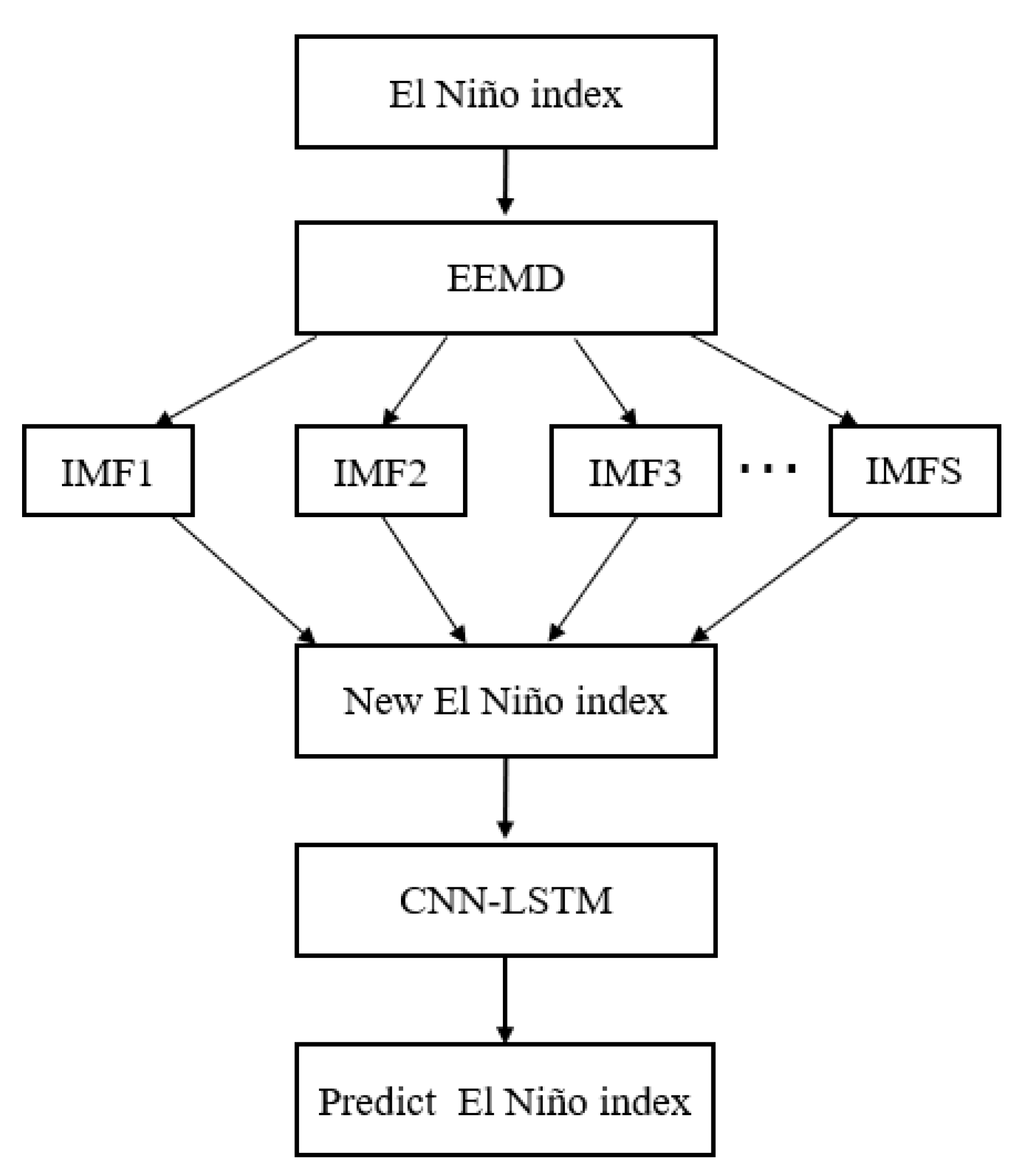
Time series generated by nonlinear dynamical systems [37,38,39] display features that cannot be modeled by linear processes: time-varying variance, higher-moment structures, asymmetric cycles, thresholds, and breaks. Different widely used ENSO indices inherit all these features [40]. The observed characteristics of ENSO are irregular and quasi-periodic, which may be caused by nonlinear dynamics or random forcing [41,42,43]. Although there are multiple El Niño indices, in this study, we selected the Nino 3.4 index for the study, and in future studies, we will also analyze other indices. Suppose that we have access to the El Niño index series: , where represents the El Niño index value at the time point. Based on historical information, a good forecasting model can make accurate predictions about the value of future moments. In this study, the basic idea of El Niño index prediction is consistent with the general time series prediction approach, which uses historical data to predict future states. The historical data were first decomposed using the EEMD method, and then the new time series were obtained using the reconstruction method. CNN was used for feature extraction and the CNN results were put into the LSTM for training to predict the future El Niño index. The overall algorithm flow is shown in Figure 1.
2.2. Ensemble Empirical Mode Decomposition
Empirical Mode Decomposition (EMD) is a signal analysis method proposed by Huang in 1998 [44]. It decomposes a complex sequence into several different scales of the Intrinsic Mode Function (IMF) and a residual component to obtain a smooth sequence. EMD avoids the selection of small wave base functions and is widely used in non-smooth signal processing. EMD is very good at handling non-stationary and non-linear time series. In contrast to other time–space analysis methods, such as wavelet decomposition, EMD is also not physics-based. However, the results of EMD decomposition can reflect much of the essential information contained in the original time series. In particular, the method is very effective for analyzing non-linear and non-stationary signals in nature, such as the Southern Oscillation Index (SOI), Nino 3.4 index, etc. [45]. However, there is a mode mixing phenomenon in the EMD method; therefore, Wu and Huang proposed the Ensemble Empirical Mode Decomposition (EEMD) algorithm [46]. The EEMD algorithm first adds white noise to the original time series and then uses the EMD method to decompose the new signal. All modes are averaged to get the final results. The specific steps of the EEMD algorithm are as follows:
Step 1: White noise satisfying a normal distribution is added to the time series X(t):
Step 2: The new time series is decomposed using the EMD algorithm to find all IMF components and one residual component .
Step 3: Repeat steps 1 and 2, adding a new white noise sequence each time.
Step 4: The decomposition results are averaged, and the average is used as the final IMF component of sequence X(t):
Based on the residuals and a series of IMFs, the energy value of each IMF was calculated as follows:
We get by summing all , i.e., , . The threshold is defined as the ratio of the energy value of the IMF to all energy.
Here, we set the threshold value . When is greater than , it indicates that the component corresponding to has an important role and cannot be ignored in signal reconstruction. Therefore, we select several that satisfy to reconstruct the new time series. These selected have more valid information, while the that does not meet the conditions is noise. Finally, we get the new reconstructed time series.
In addition, the amplitude of added noise and the ensemble number are two key parameters that affect EMMD performance. The choice of these two parameters will affect the mode decomposition results, which will affect . In this study, the amplitude and ensemble numbers mentioned above are set to 0.04 and 100, respectively, based on the results of previous studies [47,48,49] and the characteristics of the Nino 3.4 index time series.
2.3. Long Short-Term Memory Neural Network
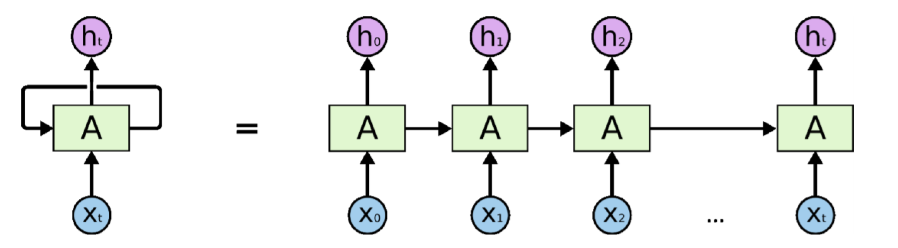
Since traditional neural networks cannot remember information, they cannot effectively use the historical information contained in the time series. Compared to traditional neural networks, the Recurrent Neural Network can remember information because the current output depends on previous calculations. In traditional neural networks, all inputs are independent of each other; however, in RNN, all inputs are interrelated. Due to its advantages in processing sequence information, RNN is widely used in text classification, machine translation, speech recognition, etc. [50]. The structure of the RNN can be seen in Figure 2.
In Figure 2, we can see the decomposition structure of a Recurrent Neural Network, and it can be found that each moment’s information can be passed to the next moment. is the input value for moment . The formula for the current state is: . As can be seen from Figure 2, the input value is first provided to the RNN, and then the output can be obtained, which together with serves as the next input. Similarly, will serve as the next input along with , and so on. In this way, the RNN can continuously memorize the context during the training process. However, when dealing with long time series, RNNs suffer from problems such as gradient disappearance. LSTM is designed to tackle these problems.
LSTM has evolved on the basis of RNN and has achieved desirable results in many areas. LSTM is especially ideal for addressing the problem of time series forecasting, as it has a versatile potential to manage critical events with longer periods and time series delays.
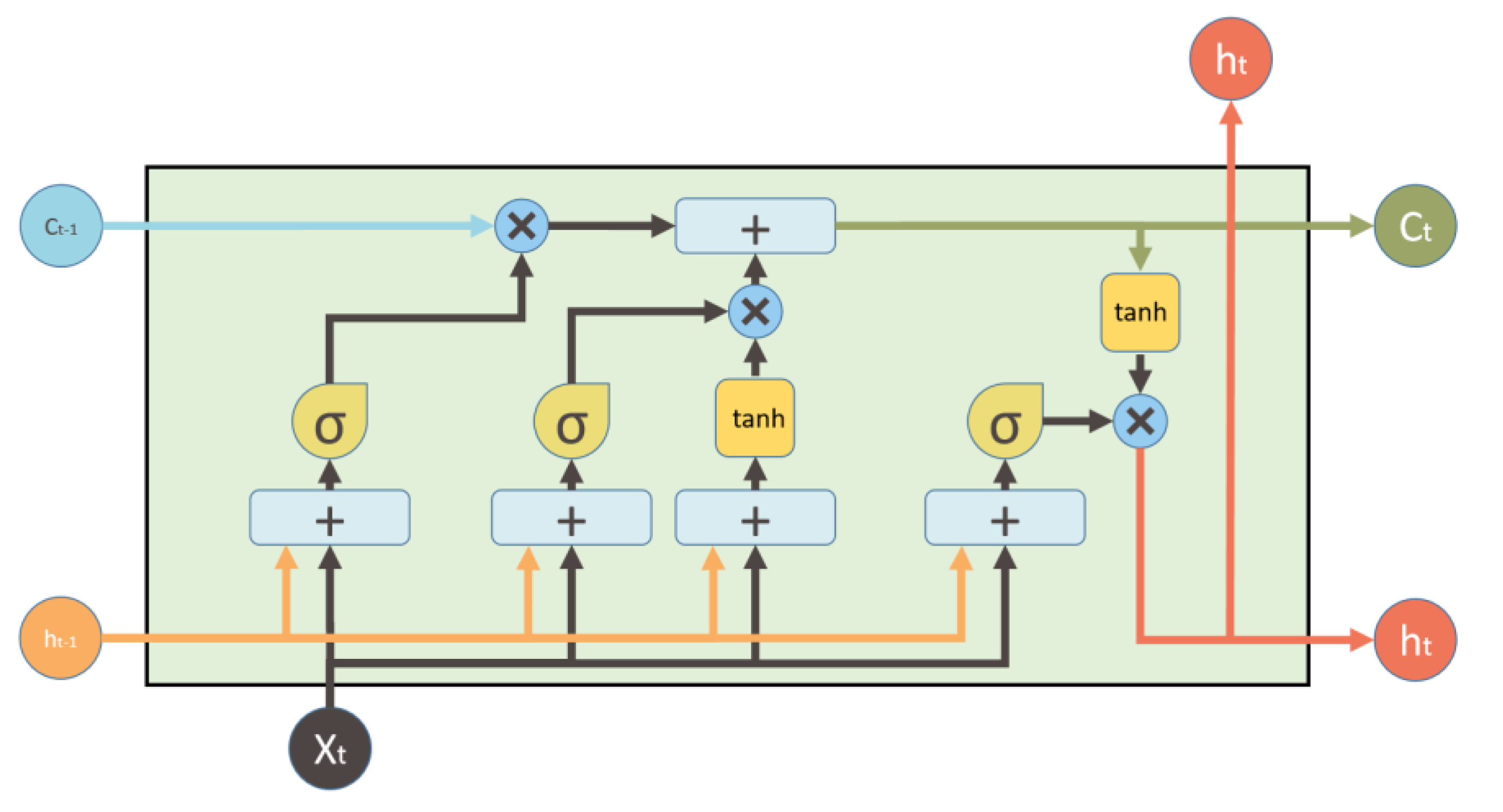
LSTM effectively overcomes the vanishing gradients problem of the RNN model by retaining useful information and discarding useless information. The structure of the LSTM can be seen in Figure 3. The LSTM mainly consists of the memory cell and three gates, including the input gate, forget gate, and output gate. These three gates take on the task of updating, maintaining, and deleting information contained in cell status. The LSTM employs the recurrence to represent the input data :
where represents the input data at time t, and and represent the hidden states computed at time t−1 and t, respectively.
- (1)
- According to Equation (7), the input and are processed to determine whether to forget the data acquired at the previous moment based on the results of the calculation.
- (2)
- According to Equation (8), the information to be stored in the cell state is calculated. At the same time, according to Equation (9), the input gate is used to determine which input data can be collected in the cell.
- (3)
- Based on Equation (10), the results of steps 1 and 2 are processed to filter out the useless data and absorb the useful ones.
- (4)
- Based on the output gate, this step determines the results of the model. Specifically, according to Equations (11) and (12), the output gate determines whether the latest cell output can be passed forward.
- (5)
- Then repeat the above steps continuously. Finally, the parameters in the LSTM are obtained by maximizing the similarity between the target data and the LSTM output.
2.4. Temporal Convolutional Neural Network
Spatiotemporal data analysis is an emerging area of research due to the development and application of new computational techniques that enable the analysis of large spatiotemporal databases [54,55]. Spatiotemporal data analysis methods can improve the utilization of our data, and this type of analysis method has been greatly developed in recent years [56,57]. Some applications of spatiotemporal analysis include cases in agriculture, oceanography, meteorology, biology, etc. Convolutional Neural Network (CNN) is a very effective method for spatiotemporal data analysis. The CNN is a feedforward neural network that evolved from the Multilayer Neural Network (MLNN). Unlike the traditional MLNN, CNN enables parameter sharing and sparsity. Specifically, since the traditional MLNN uses a full-connection strategy, each output neuron generates connections to each input neuron. For example, if there are inputs and outputs, the weight matrix will have elements. Whereas CNN uses a convolutional kernel of size k × k to reduce the size of the weight matrix from m × n to k × n. In addition, since the convolutional kernel is shared by all inputs, only a weight matrix of size k × n is learned during the training process. The training efficiency of parameter optimization is significantly improved, and CNN can train neural networks with more hidden layers at the same computational complexity. Thus, CNN can train deeper neural networks and effectively extract useful information from training data, greatly improving the quality of the model. Convolutional neural networks have achieved great success in image recognition and image classification, and today, it is used in many fields [58,59].
In order to better extract useful information from the univariate time series, a temporal convolutional neural network is proposed on the basis of traditional CNN. The traditional convolutional neural networks use a k × k convolutional kernel, but the temporal convolutional neural networks use a kernel size of k × 1. The parameter k is kernel size and it is indeed an important parameter of the temporal convolutional neural network to tune. The kernel size determines the length of the time series for each read, and then the convolution operation extracts the information contained in the reading of time series. Readings may not be accurate enough for larger kernel size, but it is possible to get an overview of the overall time-series information. We set up a comparison experiment to pick the right kernel size, and different kernel sizes were chosen for the experiment, including kernel sizes from 3 to 10. The results show that proper kernel size does lead to better accuracy, and it was found that kernels with a kernel size of 6 can achieve better results. Therefore, we set the value of the kernel size to 6. A kernel is a matrix of weights that are multiplied with the input to extract relevant features. In 2D convolutions, the kernel matrix is a two-dimensional matrix. In temporal convolutions, the kernel matrix is a one-dimensional matrix. First, suppose the input sequence fits function . Besides, the convolutional kernel function is , which is a vector of length k and it is constantly updated during the training. It should be noted that the variables of these functions are discrete moments, and their definition domains are discontinuous. Specifically, w(t) is the time series of the input, and the convolutional kernel function f(t) is a vector of parameters that are adapted by the learning algorithm. Specifically, if the step size is q, then the one-dimensional convolutional mapping between the input and kernel can be expressed as follows:
2.5. CNN-LSTM Forecasting Framework
First, in the data pre-processing phase, the temporal CNN is used to extract important information from the input data. The key point is the use of convolution to reconstruct univariate input data into multidimensional data for reorganization. In order to maximize the retention of extracted features, we omitted the merge operation.
Next, in the second phase, the features extracted in the first phase using temporal CNN were entered into the LSTM model as training data. A large number of studies have shown that training models are prone to overfitting when training data is limited [61]. The model generally takes the form of an overly complex model to explain the features and patterns in the data under study. Since we only have data with a length of forty years, the training model is prone to overfitting during training. Therefore, in this study, we use dropout to prevent overfitting. During the training, a set of dropout rates was selected for comparison. The training was conducted with a dropout rate of 0.01, 0.05, 0.1, 0.2, 0.3, 0.4, 0.5, and it was found that the training was better when the dropout rate was equal to 0.2. Therefore, the dropout rate is chosen as 0.2. In order to optimize the weights of all LSTM units, it is necessary to calculate the difference between the predicted result and the true value and obtain the loss value. Weight optimization of deep neural networks is key to the training process. Different gradient descent algorithms such as Stochastic Gradient Descent (SGD) and Adaptive Moment Estimation (Adam) were used to optimize the experiment.
2.6. A Multi-Step El Niño Index Forecasting Strategy
For the prediction of climate indices, the results of short predictions are of little significance and therefore require multi-step long time-series predictions. Although the raw El Niño data has a step size of 1 day, it can be reconstituted into different data sets with step sizes of n days, 2*n days,..., k*n days. In the study, we focus on data sets with n = 10. Newly predicted indices are used as historical data in the forecasting process, and new forecasts are continually made to predict the El Niño index for the next 10 days, 20 days... to 10 k days.
3. Experiment Design and Evaluation Methods
3.1. Dataset and Preprocessing
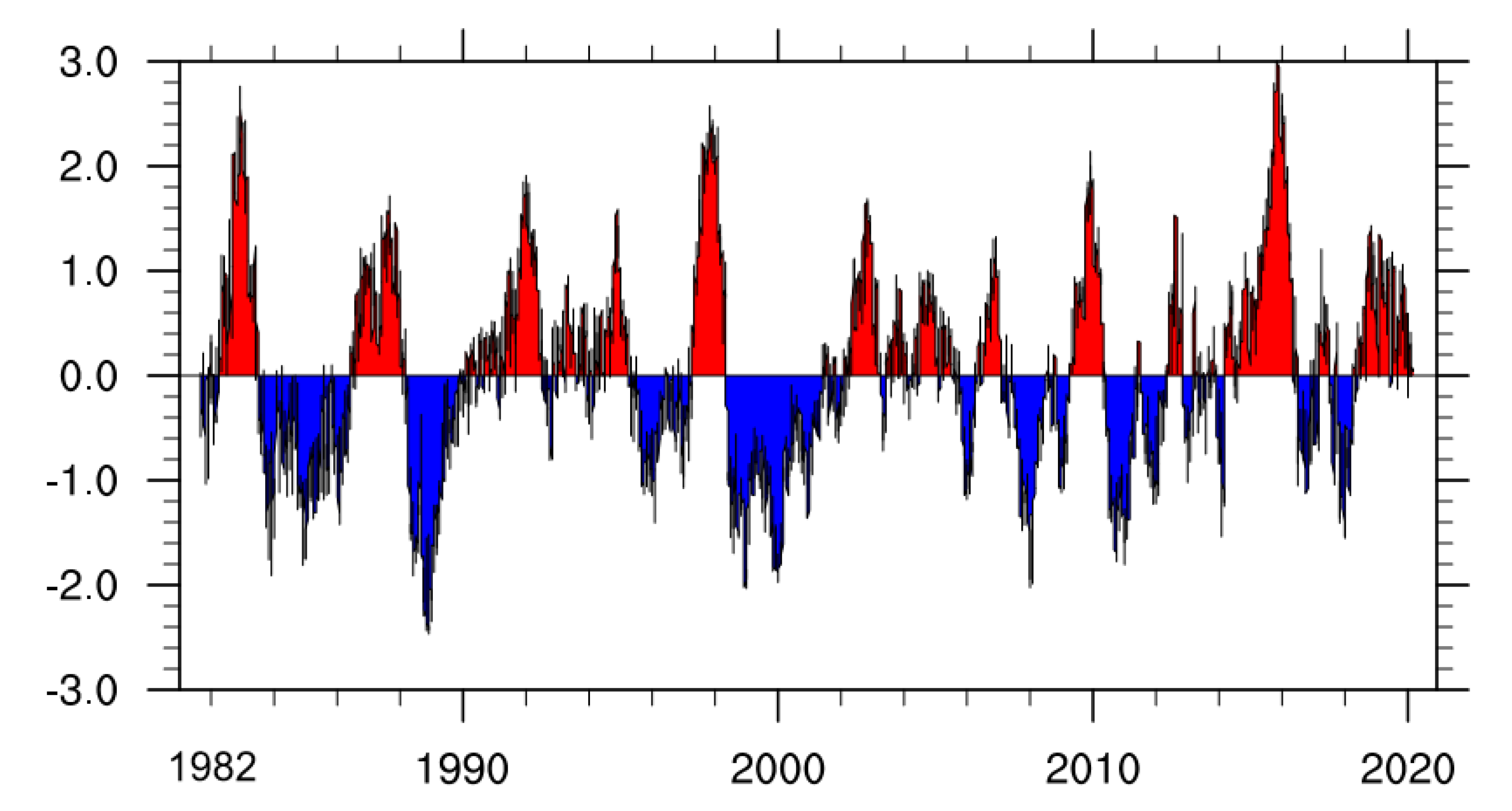
The dataset was the El Niño index (Nino 3.4 index) data, which were supplied by the Royal Netherlands Meteorological Institute (KNMI) [62]. In this study, we used daily data from 1 September 1980, to 29 February 2020. The dataset contains 14,061 samples, and we use the first 12,176 samples as the training set and the remaining data as the test set. For both the training set and the testing set, we first process the data using the EEMD method, then process the reconstructed data using the CNN, and finally input the CNN results into the LSTM. Table 1 shows descriptive statistics for this dataset. The original El Niño index series in the experiment is shown in Figure 5.
The original time series needs to be normalized before it can be entered into the model. The normalization method we chose was min–max normalization, which is one of the most frequently used normalization methods. For each feature, the minimum value of that feature is converted to 0, the maximum value is converted to 1, and all other values are converted to non-negative decimals between 0 and 1. This is a pre-processing method that performs a linear transformation of the raw data. The specific formula is as follows:
where and are the maximum and minimum values of the original sequence, respectively. After the prediction is completed, the predicted value needs to be anti-normalized to get the true value. The specific conversion function is as follows:
3.2. Parameters Details
A reasonable threshold parameter needs to be selected for time series noise reduction using the EEMD method. In order to obtain the optimal threshold, multiple sets of experiments were conducted for analysis, and the results are shown in Table 2, where MAE is Mean Absolute Error, RMSE is Root Mean Squared Error, and EV is Explained Variance. We find that the threshold value for white Gaussian noise is optimal. By comparison, it can be found that if the threshold is too small, it introduces useless IMFs that are not conducive to signal reconstruction. If the threshold value is greater than 0.04, then the IMF reflecting the original time series is discarded.
Our implementation was based on the Tensorflow framework [63]. To prevent the problem of gradient explosion during training, we made the model training more robust by reducing the learning rate and increasing the number of batches. The process of model training is to minimize the loss function, so after defining the loss function, setting up a suitable optimizer to solve the parameter optimization problem is very important for experimental results. There is a great number of optimization algorithms to choose from in current deep learning libraries, such as Stochastic Gradient Descent (SGD) and Root Mean Square Prop (RMSProp). The ideal optimizer can not only get the best model as fast as possible with the training samples but also prevent overfitting. In order to choose the best optimizer, we have carried out comparative experiments, which compared the Mean Squared Error (MSE) loss of different optimizers when training the EEMD-CNN-LSTM model. From comparative experiments, we found that the Adam method is the best. Adam has been widely used as an effective stochastic optimization method. Therefore, Adam optimizer is used in the process of training the model, which can converge to good results faster. The Rectified Linear Unit (ReLU) does not have any backpropagation error compared to the sigmoid function. And for larger neural networks, it is faster to build models based on ReLU. Therefore, when selecting the activation function in the experiment, we chose ReLU as the activation function. In this study, the input of CNN-LSTM is 100 × 1 data. There is a variable consisting of a 100-day time series. The data passes through the convolution layer and then through the LSTM. For each convolution layer, the number of filters was set to 256, the kernel size was set to 6 × 1, and the stride number was set to 1. Moreover, we applied dropout to the LSTM and set the dropout rate to 0.2 to prevent overfitting.
3.3. Evaluation of Experiments
In this experiment, Root Mean Square Error (RMSE), Mean Absolute Error (MAE), and Mean Absolute Percentage Error (MAPE) were selected to evaluate the error. The corresponding formulas are given as follows:
where and are the true value and the prediction at time , respectively. N represents the total number of samples tested. MAE, MAPE, and RMSE can reflect forecast performance, with small values indicating good forecast results.
For the traditional statistical models, such as the Autoregressive Integrated Moving Average model (ARIMA), the training process is done based on fixed mathematical formulas, and if the training data set does not change, then the model of the training does not change either, resulting in the same predicted results. Besides, we performed multiple forecast tests using LSTM, CNN-LSTM, and EEMD-CNN-LSTM to analyze the stability of the model’s forecast results. Finally, we evaluated the predictive performance of these models by analyzing the changes in RMSE and correlation skills over time.
4. Experiments Result and Analysis
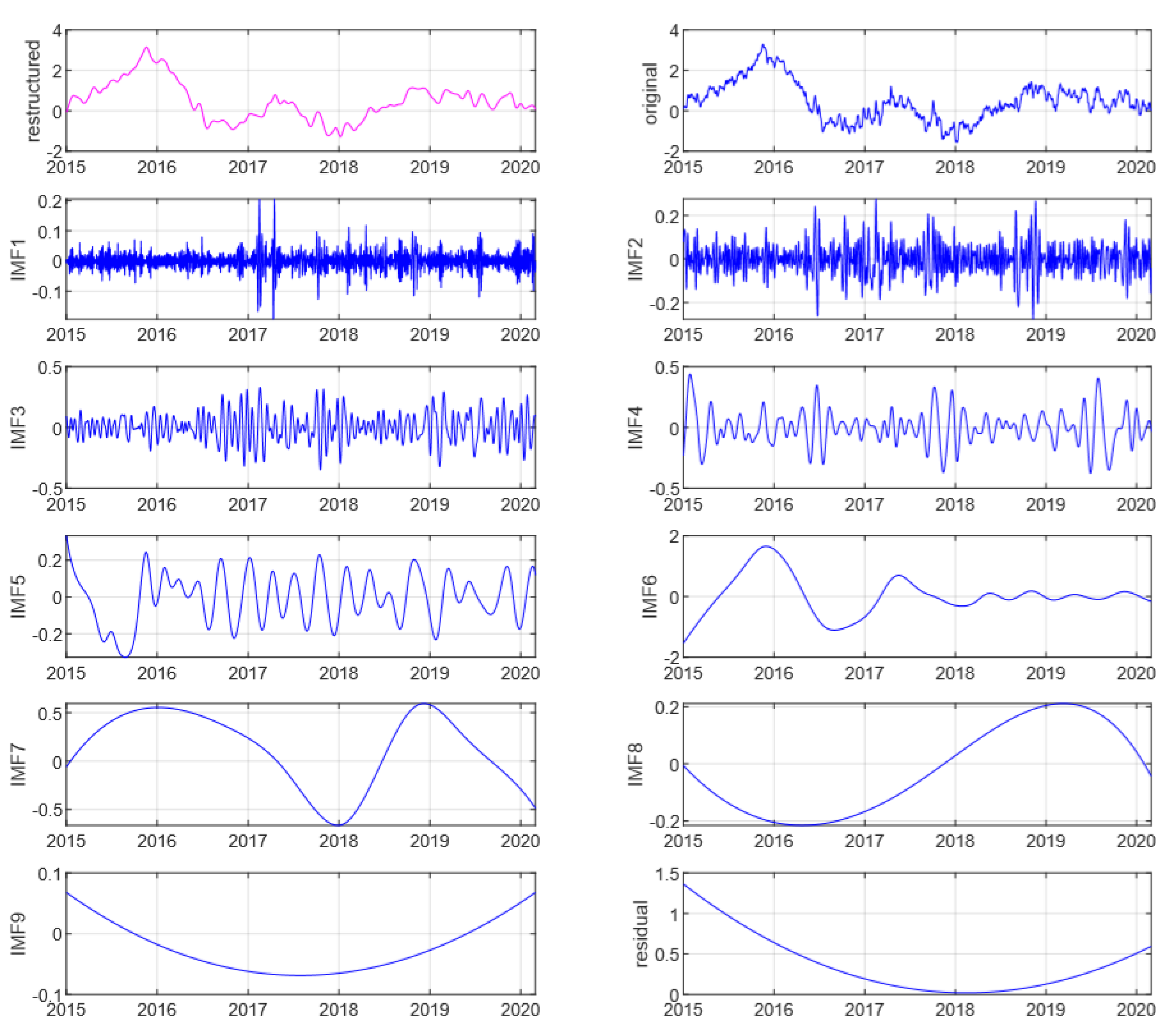
First, the EEMD method is used to eliminate the noise of the original El Niño index time series. The amplitude and ensemble number of the added noise are 0.04 and 100, respectively. Figure 6 shows the IMFs and residual of the EEMD decomposition, as well as the original and reconstructed sequences. The Nino 3.4 index in Figure 6 is day by day, and we used the EEMD method to process the time series on the entire interval. From Figure 6, it can be seen that the fluctuation frequency decreases gradually from IMF1 to IMF10. According to Equations (4) and (5), the energy values of IMFs are calculated. Next, IMFs with energy values greater than a threshold are selected to reconstruct the time series. The left side of the first row of Figure 6 shows the reconstructed Nino 3.4 index time series (purple line), the right side of the first row shows the original Nino 3.4 index time series (blue line), and the rest are IMFs and residual. In Figure 6, the reconstructed time series is smoother. To critically analyze the effect of the EEMD method, we calculated the variance of the time series before and after using the EEMD method. We finally obtained a variance of 0.9104 for the original time series and 0.8712 for the reconstructed time series, indicating that the EEMD method can effectively filter out high-frequency signal interference and thus provide good historical data for prediction.
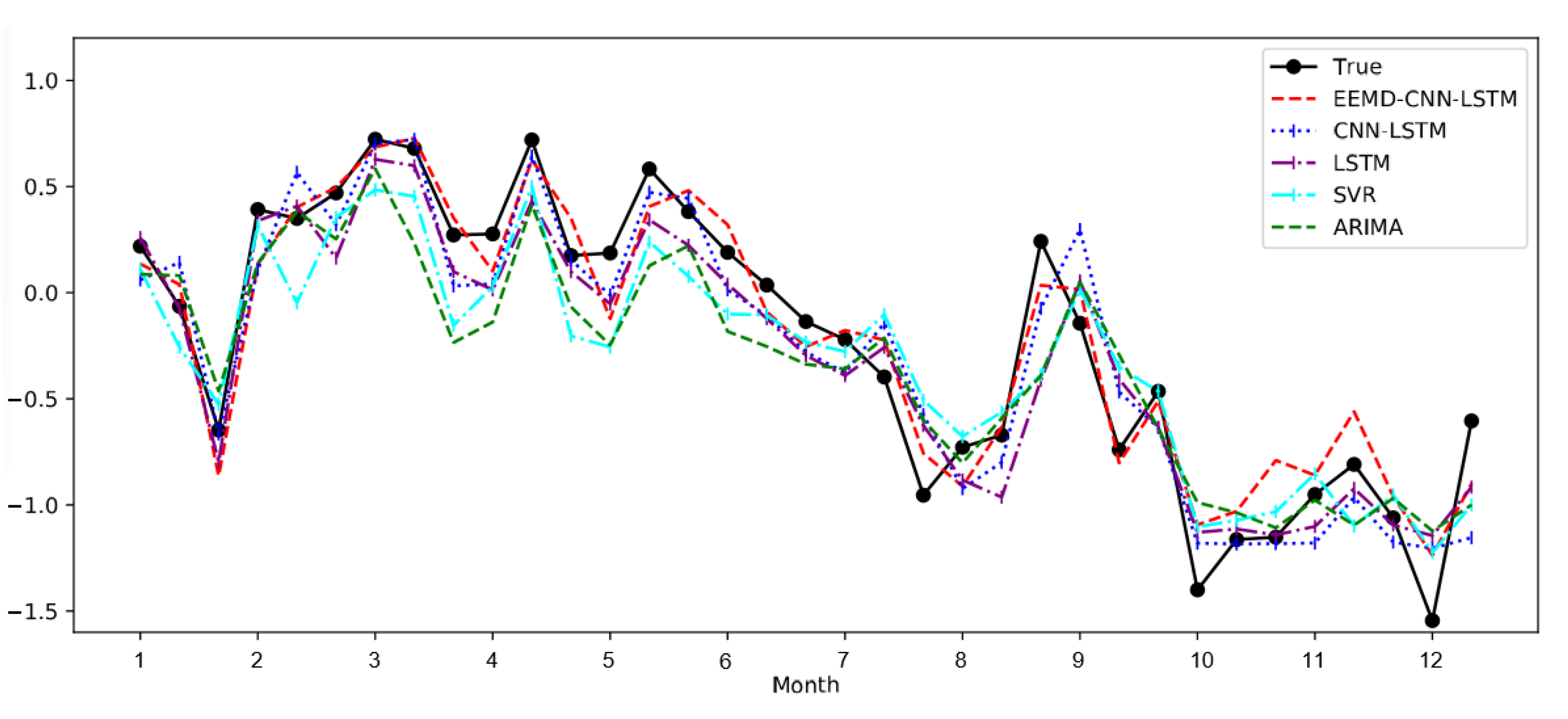
We then used the newly reconstructed data to train the hybrid neural network model. The time interval between the raw data is one day. However, during the training and prediction process, we took the real data from the last 100 days as input and output the predicted results for the next 10 days, and the predicted results were still daily. During the forecasting process, we take the forecast results as historical data and continue to forecast forward, so we can get forecasts that are months to a year in length. To test the effectiveness of this model, we compared it with four other prediction models, including the Autoregressive Integrated Moving Average model (ARIMA), Support Vector Regression (SVR), LSTM model, and CNN-LSTM model. To analyze the performance of different models, a line chart is drawn to visualize the forecast results of different models. Specifically, Figure 7 shows the 12 month forecast results and true values for 2017. The time interval for the forecast results in Figure 7 is 10 days. As can be seen from the figure, the predicted values of the EEMD-CNN-LSTM model are closer to the real values. For other models, especially traditional statistical models, they have large errors, while the EEMD-CNN-LSTM model has a similar trend to the true time series and has small prediction errors.
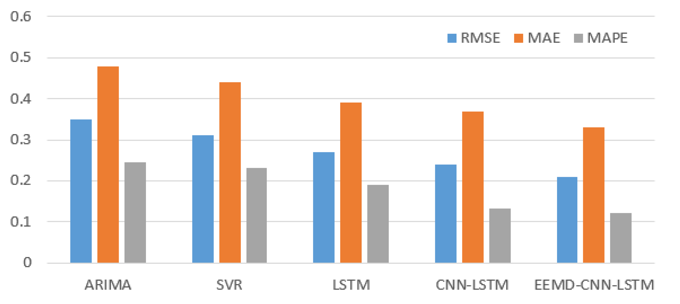
In order to study the performance of the proposed method, a rigorous quantitative analysis of the predicted and actual results was performed. We conducted a quantitative analysis of the 2017 forecast results. The error statistics show that the EEMD-CNN-LSTM model has significant advantages. To more visually demonstrate the differences between the different models and the superiority of the proposed methods, we have drawn histograms to show the predicted results. The MAE, RMSE, and MAPE values for the different prediction models are shown in Figure 8.
Based on the specific statistical results and Figure 8, we get the following results: the MAPE value of EEMD-CNN-LSTM presented in this paper is 12.20%, while those of ARIMA, SVR, LSTM and CNN-LSTM are 24.63%, 23.07%, 19.15%, and 13.17%, respectively. Besides, the RMSE values of ARIMA, SVR, LSTM, CNN-LSTM, and the proposed method are 0.35, 0.31, 0.27, 0.24, and 0.21, respectively. The MAE value for the EEMD-CNN-LSTM model is 0.33, which is also smaller than that obtained by ARIMA, SVR, LSTM, and CNN-LSTM, which are 0.48, 0.44, 0.39, and 0.37, respectively.
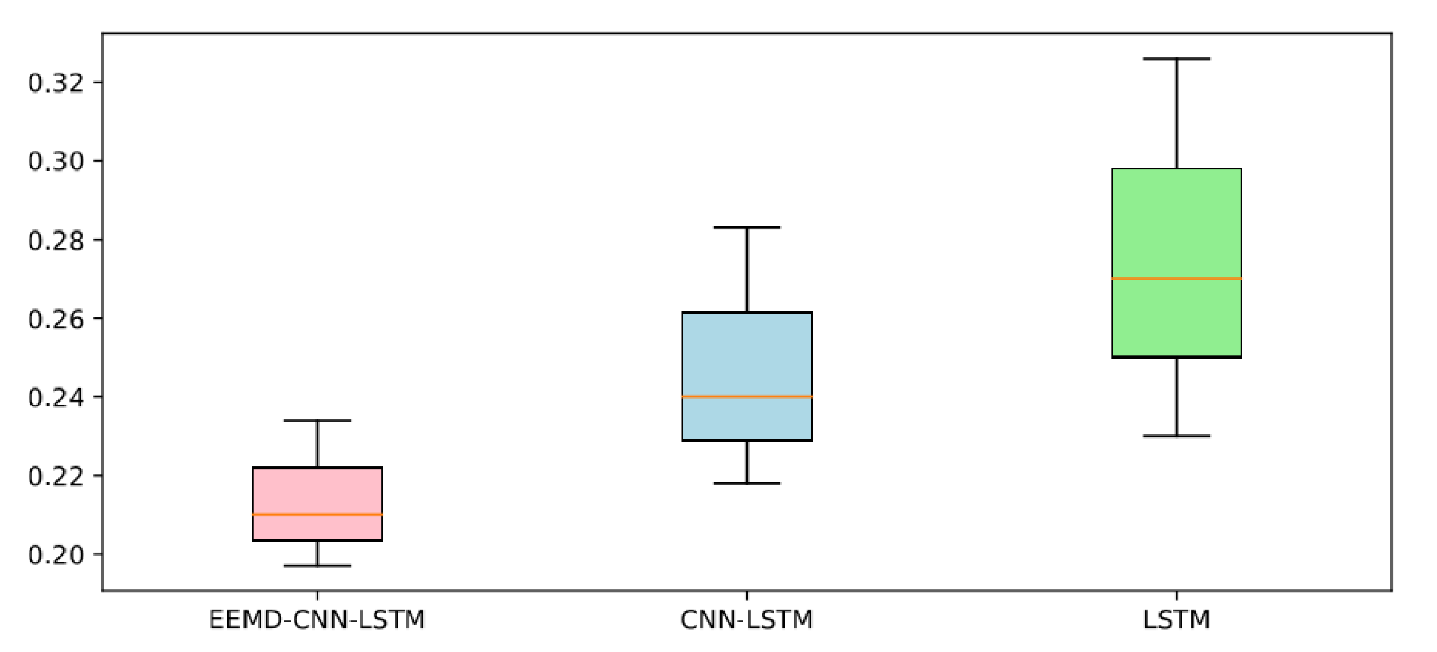
Finally, we also performed a robust comparative analysis of the three LSTM models. Figure 9 shows the RMSE distribution of the predicted results for EEMD-CNN-LSTM, CNN-LSTM, and LSTM. As shown in Figure 9, the median, maximum, and minimum values of the RMSEs for the different models correspond to the red lines and the top and bottom rows of the box. From Figure 9, it is found that EEMD-CNN-LSTM has the lowest RMSE and reliable stability for time series prediction.
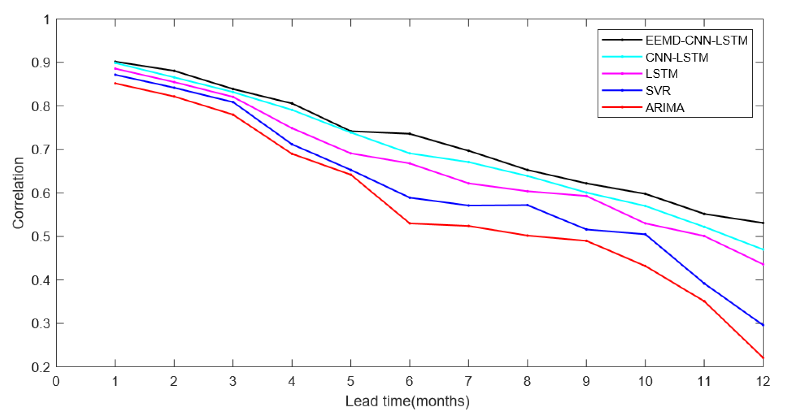
In order to study how the forecast skill changes with prediction time, we analyzed the temporal correlation between the forecast results and the actual data for all seasons combined [64,65,66]. We found that the temporal correlation changes significantly with lead time. The analysis process is based on the test data set for the period 2015 to 2020. The correlation between model forecasts and observations reflects the different abilities of the prediction models. Figure 10 shows different model correlation skills that change over lead time. In the beginning, the correlation skills of the models appear roughly comparable. However, the forecast skill of the Nino 3.4 index in the Artificial Neural Network models is systematically superior to statistical models at lead times longer than three months. From the results of the analysis, it can be concluded that the neural network-based prediction model has good results and the hybrid model is better than the single LSTM model. The above results show that the neural network-based hybrid model has good application prospects for El Niño index prediction. However, our present study is limited to the prediction of the Nino 3.4 index, and our next work will be to predict the more complex El Niño index and the time series of sea surface temperature (SST) anomalies in two-dimensional space and analyze their forecast skills.
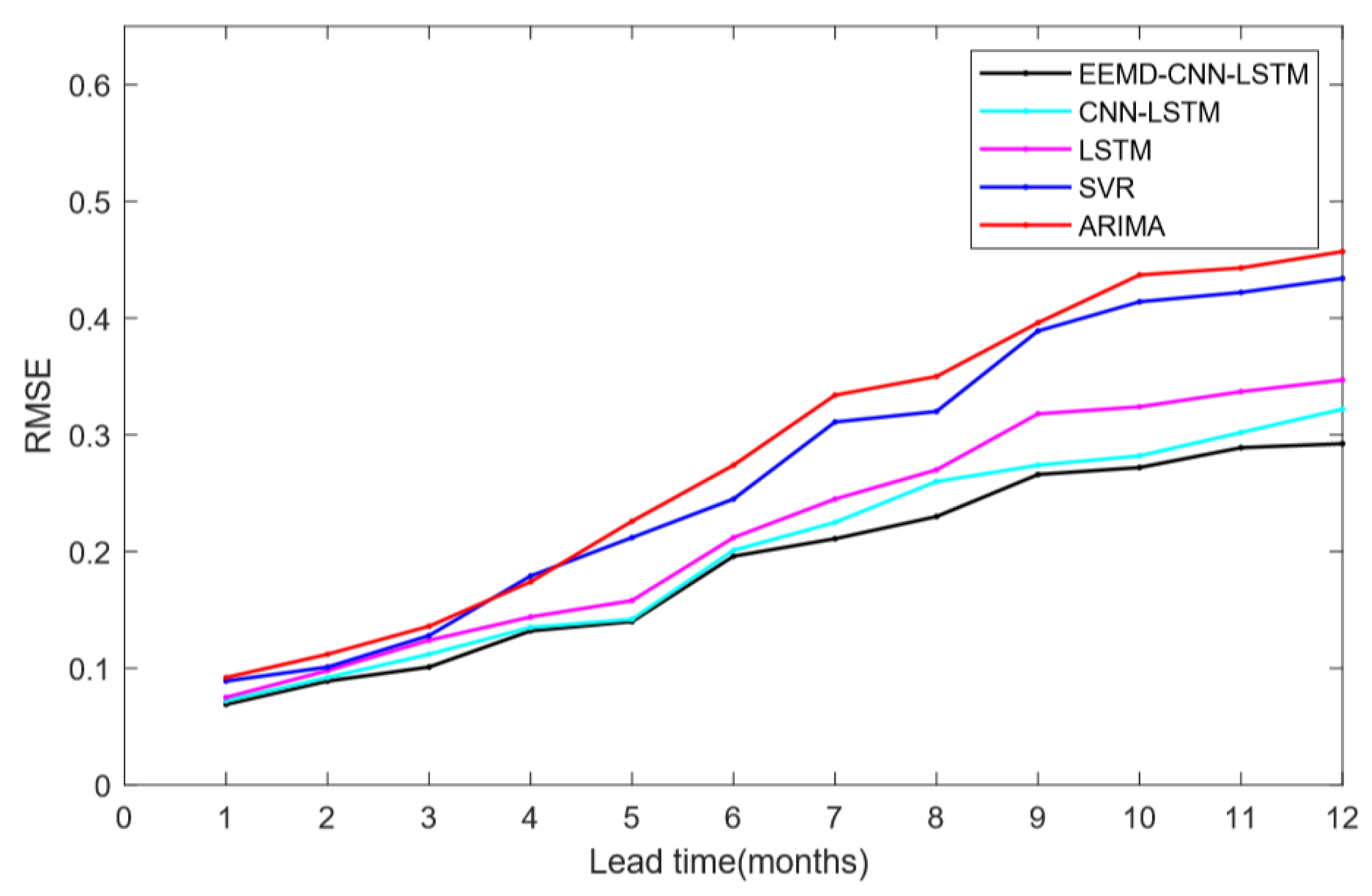
In addition, we examined the RMSE for different models to assess performance in terms of both discrimination and calibration. Figure 11 shows RMSEs which change over lead time for all seasons combined. As shown in Figure 11, the EEMD-CNN-LSTM model has the lowest RMSE over its range of lead times. We also found that for lead times greater than 3 months, the RMSE was significantly higher for non-neural network models than for neural network models. By comparing the correlation skill with Root Mean Square Error (RMSE), we found that the model with lower RMSE tended to have a higher correlation. The above results show that our proposed EEMD-CNN-LSTM model has significant advantages in predicting the Nino 3.4 index.
5. Discussions
The prediction of the El Niño phenomenon has always suffered from high volatility and uncertainty. In this study, we construct a hybrid deep learning method that combines ensemble empirical mode decomposition, temporal convolutional neural network, and LSTM to predict the El Niño index and compare it with the conventional method. From the above experimental results, it can be discussed that:
- (1)
- Based on the above experimental results, we find that the model using LSTM was significantly better than ARIMA and SVR. This suggests that LSTM has a significant advantage over conventional methods in time series prediction, especially for the prediction of climate indices with chaotic properties.
- (2)
- Compared with the single LSTM, the CNN-LSTM model has better prediction accuracy. The reason for the difference in prediction accuracy should be CNN. CNN can extract features of complex time series, thus effectively improving the performance of El Niño index predictions. Besides, the performance and robustness of the El Niño index predictions are effectively improved due to the EEMD method, which eliminates noise interference in complex nonlinear time series. However, it should also be noted that we were using the EEMD method to filter out the high-frequency noise on the training set and the test set, respectively. This may cause inconsistencies in the degree of filtering between the test set and the training set, affecting the prediction of the model and causing the training model to perform poorly on the test set. In future work, we will further investigate the use of the EEMD method and parameter optimization.
- (3)
- It is well known that the El Niño index is more random and unstable than other climate indices. However, the method proposed in this study has achieved good results in predicting the El Niño index, so the model can also be used to predict other climate indices, such as the Southern Oscillation Index, East Asian summer monsoon index, etc. In addition, it should not be overlooked that the El Niño event, as a special phenomenon in the Earth system, is inextricably linked to other climate events; hence, in the future, we will train models with data from other climate events in order to obtain better prediction models.
- (4)
- In this study, we focus on the 10 day forecast of the Nino 3.4 index. However, the forecast was not limited to 10 days, as the new forecast results were used as historical data during the forecasting process to continue the forecast forward, culminating in a year of Nino 3.4 index forecasts. In this study, for 2017, the Nino 3.4 index prediction yielded good results, and we will test the effectiveness of our model against other El Niño indices and more time in future studies. On the other hand, the predictability time is a very important parameter in the El Niño predictions. In fact, the spring predictability barrier is the great challenge of El Niño predictions. The methods presented in this study have not been studied on the issue of the spring predictability barrier, and in the future, we will adjust the forecast timing to study this issue in depth.
- (5)
- El Niño is a large-scale sea surface temperature (SST) anomaly phenomenon that is strongly spatially correlated, and the study of El Niño cannot ignore spatial information [66]. In El Niño predictions, the time scale information deficit can be addressed by using more spatial information. Our present study demonstrates that EEMD and neural network-based deep learning methods are effective in predicting indices, suggesting that they should also be useful in predicting other physical quantities of El Niño. Next, we will make predictions about the time series of SST anomalies, which is entirely possible because CNN can easily process the two-dimensional space data. Therefore, the EEMD-CNN-LSTM proposed in our paper should yield good results in the prediction of space SST anomalies.
- (6)
- It should not be overlooked that we used the EEMD method for noise reduction on the test set before making the forecast on the test set. As is known to all, any smoothing process such as EEMD transfers future information to the past, i.e., the spread of information over the entire interval. In this way, some part of the prediction improvement may be caused by the fact that the information about the future is already in the input of the predicting operator. This strategy is difficult to achieve when making real-time predictions because the future is completely unknown.
6. Conclusions
In order to predict the El Niño index more accurately, we propose a new hybrid neural network model, EEMD-CNN-LSTM, which combines Ensemble Empirical Mode Decomposition (EEMD), Convolutional Neural Network (CNN), and Long Short-Term Memory (LSTM). First, the original El Niño index time series is decomposed into many Intrinsic Mode Functions (IMFs) and a residual component using the EEMD method. Next, the reconstruction operation is performed to obtain the new El Niño index time series. Then, the new time series is used to train the hybrid neural network model, and future El Niño indices are predicted using the trained model. The experimental results show that the proposed EEMD-CNN-LSTM model has a significant advantage over the other models in this paper. We can draw the following conclusions: (a) Generally, compared to traditional statistical methods, LSTM is better suited for predicting highly complex nonlinear time series. In the experiments of El Niño index prediction, using the LSTM model can obtain higher prediction accuracy. (b) Besides, The EEMD method helps to eliminate noise in complex non-linear time series, and CNN helps extract effective information of time series, thereby effectively improving the accuracy and robustness of El Niño index prediction. (c) The EEMD method, LSTM neural network, and CNN are reasonably integrated and provide new ideas for El Niño index prediction. In conclusion, the method proposed in this paper is expected to provide a useful reference to the prediction of climate indices.
Author Contributions
Conceptualization, Y.G.; methodology, X.C.; validation, K.P.; investigation, Y.G.; writing—original draft preparation, Y.G.; supervision, B.L.; project administration, X.C. All authors have read and agreed to the published version of the manuscript.
Funding
This research was funded by the National Key R&D Program of China (Grant No.2018YFC1506704) and the National Natural Science Foundation of China (Grant No.41475094).
Conflicts of Interest
The authors declare no conflict of interest.
Abbreviations
| LSTM | Long Short-Term Memory |
| EMD | Empirical Mode Decomposition |
| EEMD | Ensemble Empirical Mode Decomposition |
| RNN | Recurrent Neural Network |
| CNN | Convolutional Neural Network |
| NAO | North Atlantic Oscillation |
| ARIMA | Autoregressive Integrated Moving Average |
| IMF | Intrinsic Mode Function |
| SVR | Support Vector Regression |
| SGD | Stochastic Gradient Descent |
| RMSProp | Root Mean Square Prop |
| Adam | Adaptive Moment Estimation |
References
- Yang, S.; Li, Z.; Yu, J.-Y.; Hu, X.; Dong, W.; He, S. El Niño–Southern oscillation and its impact in the changing climate. Natl. Sci. Rev. 2018, 5, 840–857. [Google Scholar] [CrossRef]
- Moy, C.M.; Seltzer, G.O.; Rodbell, D.T.; Anderson, D.M. Variability of El Niño/Southern Oscillation activity at millennial timescales during the Holocene epoch. Nature 2002, 420, 162–165. [Google Scholar] [CrossRef] [PubMed]
- Santoso, A.; Hendon, H.; Watkins, A.; Power, S.; Dommenget, D.; England, M.H.; Frankcombe, L.; Holbrook, N.J.; Holmes, R.; Hope, P. Dynamics and predictability of El Niño–Southern Oscillation: An Australian perspective on progress and challenges. Bull. Am. Meteorol. Soc. 2019, 100, 403–420. [Google Scholar] [CrossRef]
- Tudhope, A.W.; Chilcott, C.P.; McCulloch, M.T.; Cook, E.R.; Chappell, J.; Ellam, R.M.; Lea, D.W.; Lough, J.M.; Shimmield, G.B. Variability in the El Niño-Southern Oscillation through a glacial-interglacial cycle. Science 2001, 291, 1511–1517. [Google Scholar] [CrossRef]
- Cane, M.A. ENSO Prediction and Predictability. In Proceedings of the AGU Fall Meeting Abstracts, San Francisco, CA, USA, 12–16 December 2016. [Google Scholar]
- Chen, D.; Cane, M.A. El Niño prediction and predictability. J. Comput. Phys. 2008, 227, 3625–3640. [Google Scholar] [CrossRef]
- Timmermann, A.; An, S.-I.; Kug, J.-S.; Jin, F.-F.; Cai, W.; Capotondi, A.; Cobb, K.M.; Lengaigne, M.; McPhaden, M.J.; Stuecker, M.F. El Niño–southern oscillation complexity. Nature 2018, 559, 535–545. [Google Scholar] [CrossRef]
- Timmermann, A.; Latif, M.; Voss, R.; Grötzner, A. Northern Hemispheric interdecadal variability: A coupled air–sea mode. J. Clim. 1998, 11, 1906–1931. [Google Scholar] [CrossRef] [Green Version]
- McPhaden, M.J. Understanding and Predicting El Niño and the Southern Oscillation. New Front. Oper. Oceanogr. 2018, August 1, 653–662. [Google Scholar]
- Ren, H.-L.; Zheng, F.; Luo, J.-J.; Wang, R.; Liu, M.; Zhang, W.; Zhou, T.; Zhou, G. A Review of Research on Tropical Air-Sea Interaction, ENSO Dynamics, and ENSO Prediction in China. J. Meteorol. Res. 2020, 34, 43–62. [Google Scholar] [CrossRef]
- Tang, Y.; Zhang, R.-H.; Liu, T.; Duan, W.; Yang, D.; Zheng, F.; Ren, H.; Lian, T.; Gao, C.; Chen, D. Progress in ENSO prediction and predictability study. Natl. Sci. Rev. 2018, 5, 826–839. [Google Scholar] [CrossRef]
- Luo, J.-J.; Hendon, H.; Alves, O. Multi-year prediction of ENSO. In Proceedings of the Geophysical Research Abstracts, Vienna, Austria, 7–12 April 2019. [Google Scholar]
- Todd, A.; Collins, M.; Lambert, F.H.; Chadwick, R. Diagnosing ENSO and global warming tropical precipitation shifts using surface relative humidity and temperature. J. Clim. 2018, 31, 1413–1433. [Google Scholar] [CrossRef] [Green Version]
- Hanley, D.E.; Bourassa, M.A.; O’Brien, J.J.; Smith, S.R.; Spade, E.R. A quantitative evaluation of ENSO indices. J. Clim. 2003, 16, 1249–1258. [Google Scholar] [CrossRef]
- Kiem, A.S.; Franks, S.W. On the identification of ENSO-induced rainfall and runoff variability: A comparison of methods and indices. Hydrol. Sci. J. 2001, 46, 715–727. [Google Scholar] [CrossRef]
- Wolter, K.; Timlin, M.S. El Niño/Southern Oscillation behaviour since 1871 as diagnosed in an extended multivariate ENSO index (MEI. ext). Int. J. Climatol. 2011, 31, 1074–1087. [Google Scholar] [CrossRef]
- Kadilar, G.Ö.; Kadilar, C. Assessing air quality in Aksaray with time series analysis. In Proceedings of the AIP Conference Proceedings, Antalya, Turkey, 18–21 April 2017; Volume 1833, p. 020112. [Google Scholar]
- Lai, Y.; Dzombak, D.A. Use of the Autoregressive Integrated Moving Average (ARIMA) Model to Forecast Near-term Regional Temperature and Precipitation. Weather Forecast. 2020, 35, 959–976. [Google Scholar] [CrossRef]
- Mahsin, M. Modeling rainfall in Dhaka division of Bangladesh using time series analysis. J. Math. Model. Appl. 2011, 1, 67–73. [Google Scholar]
- Ludescher, J.; Gozolchiani, A.; Bogachev, M.I.; Bunde, A.; Havlin, S.; Schellnhuber, H.J. Improved El Niño forecasting by cooperativity detection. Proc. Natl. Acad. Sci. USA 2013, 110, 11742–11745. [Google Scholar] [CrossRef] [Green Version]
- Meng, J.; Fan, J.; Ashkenazy, Y.; Bunde, A.; Havlin, S. Forecasting the magnitude and onset of El Niño based on climate network. New J. Phys. 2018, 20, 043036. [Google Scholar] [CrossRef]
- Nooteboom, P.D.; Feng, Q.Y.; López, C.; Hernández-García, E.; Dijkstra, H.A. Using Network Theory and Machine Learning to predict El Nino. arXiv 2018, arXiv:1803.10076. [Google Scholar] [CrossRef] [Green Version]
- Meng, J.; Fan, J.; Ludescher, J.; Agarwal, A.; Chen, X.; Bunde, A.; Kurths, J.; Schellnhuber, H.J. Complexity-based approach for El Niño magnitude forecasting before the spring predictability barrier. Proc. Natl. Acad. Sci. USA 2020, 117, 177–183. [Google Scholar] [CrossRef] [Green Version]
- Tangang, F.; Hsieh, W.; Tang, B. Forecasting the equatorial Pacific sea surface temperatures by neural network models. Clim. Dyn. 1997, 13, 135–147. [Google Scholar] [CrossRef]
- Nooteboom, P.D.; Feng, Q.Y.; López, C.; Hernández-García, E.; Dijkstra, H.A. Using network theory and machine learning to predict El Niño. Earth Syst. Dyn. 2018, 9, 969–983. [Google Scholar] [CrossRef] [Green Version]
- Yuan, S.; Luo, X.; Mu, B.; Li, J.; Dai, G. Prediction of North Atlantic Oscillation index with convolutional LSTM based on ensemble empirical mode decomposition. Atmosphere 2019, 10, 252. [Google Scholar] [CrossRef] [Green Version]
- McDermott, P.L.; Wikle, C.K. Bayesian recurrent neural network models for forecasting and quantifying uncertainty in spatial-temporal data. Entropy 2019, 21, 184. [Google Scholar] [CrossRef] [Green Version]
- Kim, S.; Hong, S.; Joh, M.; Song, S.-K. Deeprain: Convlstm network for precipitation prediction using multichannel radar data. arXiv 2017, arXiv:1711.02316. [Google Scholar]
- Xingjian, S.; Chen, Z.; Wang, H.; Yeung, D.-Y.; Wong, W.-K.; Woo, W.-C. Convolutional LSTM network: A machine learning approach for precipitation nowcasting. In Proceedings of the Advances in Neural Information Processing Systems, Montreal, QC, Canada, 7–12 December 2015; pp. 802–810. [Google Scholar]
- Wong, W.-K.; Shi, X.; Yeung, D.Y.; Woo, W. A deep-learning method for precipitation nowcasting. In Proceedings of the WMO WWRP 4th International Symposium on Nowcasting and Veryshort-Range Forecast 2016, Hong Kong, China, 25–29 July 2016. [Google Scholar]
- Shen, H. Seasonal prediction of summer precipitation in China based on deep learning. In Proceedings of the AGU Fall Meeting Abstracts, Washington, DC, USA, 10–14 December 2018. [Google Scholar]
- Zhang, Q.; Wang, H.; Dong, J.; Zhong, G.; Sun, X. Prediction of sea surface temperature using long short-term memory. IEEE Geosci. Remote Sens. Lett. 2017, 14, 1745–1749. [Google Scholar] [CrossRef] [Green Version]
- Stratigakos, A.C.; Papaioannou, G.P.; Bachoumis, A.N.; Dikaiakos, C. Short-Term Load Forecasting with Singular Spectrum Analysis and LSTM Neural Networks. Available online: https://www.researchgat-e.net/publication/336739325_ShortTerm_Load_Forecasting_with_Singular_Spectrum_Analysis_and_LST-M_Neural_Networks (accessed on 18 May 2020).
- Wang, W.-C.; Chau, K.-W.; Xu, D.-M.; Chen, X.-Y. Improving forecasting accuracy of annual runoff time series using ARIMA based on EEMD decomposition. Water Resour. Manag. 2015, 29, 2655–2675. [Google Scholar] [CrossRef]
- Mohan, N.; Soman, K.; Kumar, S.S. A data-driven strategy for short-term electric load forecasting using dynamic mode decomposition model. Appl. Energy 2018, 232, 229–244. [Google Scholar] [CrossRef]
- Mann, J.; Kutz, J.N. Dynamic mode decomposition for financial trading strategies. Quant. Financ. 2016, 16, 1643–1655. [Google Scholar] [CrossRef] [Green Version]
- Basharat, A.; Shah, M. Time series prediction by chaotic modeling of nonlinear dynamical systems. In Proceedings of the 2009 IEEE 12th International Conference on Computer Vision, Kyoto, Japan, 27 September–4 October 2009; pp. 1941–1948. [Google Scholar]
- Kantz, H.; Schreiber, T. Nonlinear Time Series Analysis; Cambridge University Press: Cambridge, UK, 2004; Volume 7. [Google Scholar]
- Ozaki, T. A bridge between nonlinear time series models and nonlinear stochastic dynamical systems: A local linearization approach. Stat. Sin. 1992, 113–135. [Google Scholar]
- Hall, A.D.; Skalin, J.; Teräsvirta, T. A nonlinear time series model of El Nino. Environ. Model. Softw. 2001, 16, 139–146. [Google Scholar] [CrossRef]
- Chang, P.; Wang, B.; Li, T.; Ji, L. Interactions between the seasonal cycle and the Southern Oscillation-Frequency entrainment and chaos in a coupled ocean-atmosphere model. Geophys. Res. Lett. 1994, 21, 2817–2820. [Google Scholar] [CrossRef]
- Tziperman, E.; Stone, L.; Cane, M.A.; Jarosh, H. El Nino chaos: Overlapping of resonances between the seasonal cycle and the Pacific ocean-atmosphere oscillator. Science 1994, 264, 72–74. [Google Scholar] [CrossRef] [PubMed] [Green Version]
- An, S.-I.; Jin, F.-F. Nonlinearity and asymmetry of ENSO. J. Clim. 2004, 17, 2399–2412. [Google Scholar] [CrossRef]
- Huang, N.E.; Shen, Z.; Long, S.R.; Wu, M.C.; Shih, H.H.; Zheng, Q.; Yen, N.-C.; Tung, C.C.; Liu, H.H. The empirical mode decomposition and the Hilbert spectrum for nonlinear and non-stationary time series analysis. Proc. R. Soc. Lond. Ser. A Math. Phys. Eng. Sci. 1998, 454, 903–995. [Google Scholar] [CrossRef]
- Juanxiong, H.; Zhihao, Y.; Xiuqun, Y. Temporal characteristics of Pacific Decadal Oscillation (PDO) and ENSO and their relationship analyzed with method of Empirical Mode Decomposition (EMD). J. Meteorol. Res. 2004, 19, 83–92. [Google Scholar]
- Wu, Z.; Huang, N.E. Ensemble empirical mode decomposition: A noise-assisted data analysis method. Adv. Adapt. Data Anal. 2009, 1, 1–41. [Google Scholar] [CrossRef]
- Lei, Y.; He, Z.; Zi, Y. Application of the EEMD method to rotor fault diagnosis of rotating machinery. Mech. Syst. Signal Process. 2009, 23, 1327–1338. [Google Scholar] [CrossRef]
- Ma, Z.; Wen, G.; Jiang, C. EEMD independent extraction for mixing features of rotating machinery reconstructed in phase space. Sensors 2015, 15, 8550–8569. [Google Scholar] [CrossRef] [Green Version]
- Shen, Z.; Wang, Q.; Shen, Y.; Jin, J.; Lin, Y. Accent extraction of emotional speech based on modified ensemble empirical mode decomposition. In Proceedings of the 2010 IEEE Instrumentation & Measurement Technology Conference Proceedings, Austin, TX, USA, 3–6 May 2010; pp. 600–604. [Google Scholar]
- Miao, Y.; Gowayyed, M.; Metze, F. EESEN: End-to-end speech recognition using deep RNN models and WFST-based decoding. In Proceedings of the 2015 IEEE Workshop on Automatic Speech Recognition and Understanding (ASRU), Scottsdale, AZ, USA, 13–17 December 2015; pp. 167–174. [Google Scholar]
- Huang, Y.; Liu, S.; Yang, L. Wind speed forecasting method using EEMD and the combination forecasting method based on GPR and LSTM. Sustainability 2018, 10, 3693. [Google Scholar] [CrossRef] [Green Version]
- Liu, H.; Mi, X.-W.; Li, Y.-F. Wind speed forecasting method based on deep learning strategy using empirical wavelet transform, long short term memory neural network and Elman neural network. Energy Convers. Manag. 2018, 156, 498–514. [Google Scholar] [CrossRef]
- Ismail, S.; Ahmad, A. Recurrent neural network with back propagation through time algorithm for Arabic recognition. In Proceedings of the 18th ESM Magdeburg, Magdeburg, Germany, 13–16 June 2004; pp. 13–16. [Google Scholar]
- Meng, B.; Liu, X.; Wang, X. Human action recognition based on quaternion spatial-temporal convolutional neural network and LSTM in RGB videos. Multimed. Tools Appl. 2018, 77, 26901–26918. [Google Scholar] [CrossRef]
- Wu, Z.; Wang, X.; Jiang, Y.-G.; Ye, H.; Xue, X. Modeling spatial-temporal clues in a hybrid deep learning framework for video classification. In Proceedings of the 23rd ACM International Conference on Multimedia, Reykjavik, Iceland, 4–6 January 2017; pp. 461–470. [Google Scholar]
- Covas, E.; Benetos, E. Optimal neural network feature selection for spatial-temporal forecasting. Chaos Interdiscip. J. Nonlinear Sci. 2019, 29, 063111. [Google Scholar] [CrossRef] [PubMed] [Green Version]
- López, C.; Álvarez, A.; Hernández-García, E. Forecasting confined spatiotemporal chaos with genetic algorithms. Phys. Rev. Lett. 2000, 85, 2300. [Google Scholar] [CrossRef] [Green Version]
- Hijazi, S.; Kumar, R.; Rowen, C. Using Convolutional Neural Networks for Image Recognition; Cadence Design Systems Inc.: San Jose, CA, USA, 2015; pp. 1–12. [Google Scholar]
- Li, Q.; Cai, W.; Wang, X.; Zhou, Y.; Feng, D.D.; Chen, M. Medical image classification with convolutional neural network. In Proceedings of the 2014 13th International Conference on Control Automation Robotics & Vision (ICARCV), Singapore, 10–12 December 2014; pp. 844–848. [Google Scholar]
- Yan, K.; Wang, X.; Du, Y.; Jin, N.; Huang, H.; Zhou, H. Multi-step short-term power consumption forecasting with a hybrid deep learning strategy. Energies 2018, 11, 3089. [Google Scholar] [CrossRef] [Green Version]
- Srivastava, N.; Hinton, G.; Krizhevsky, A.; Sutskever, I.; Salakhutdinov, R. Dropout: A simple way to prevent neural networks from overfitting. J. Mach. Learn. Res. 2014, 15, 1929–1958. [Google Scholar]
- Puertas Orozco, O.L.; Carvajal Escobar, Y. Incidence of El Niño southern oscillation in the precipitation and the temperature of the air in Colombia, using Climate Explorer. Ingeniería Y Desarrollo 2008, 23, 104–118. [Google Scholar]
- Chen, H.-Y. Tensorflow–a system for large-scale machine learning. In Proceedings of the OSDI, Savannah, GA, USA, 1–4 November 2016; pp. 265–283. [Google Scholar]
- Barnston, A.G.; Tippett, M.K.; L’Heureux, M.L.; Li, S.; DeWitt, D.G. Skill of real-time seasonal ENSO model predictions during 2002–11: Is our capability increasing? Bull. Am. Meteorol. Soc. 2012, 93, 631–651. [Google Scholar] [CrossRef]
- Gavrilov, A.; Seleznev, A.; Mukhin, D.; Loskutov, E.; Feigin, A.; Kurths, J. Linear dynamical modes as new variables for data-driven ENSO forecast. Clim. Dyn. 2019, 52, 2199–2216. [Google Scholar] [CrossRef]
- Kondrashov, D.; Kravtsov, S.; Robertson, A.W.; Ghil, M. A hierarchy of data-based ENSO models. J. Clim. 2005, 18, 4425–4444. [Google Scholar] [CrossRef] [Green Version]
Figure 1.
The architecture of the proposed method.

Figure 2.
The structure of a Recurrent Neural Network (RNN).

Figure 3.
The structure of Long Short-Term Memory Neural Network (LSTM).

Figure 4.
Training data preprocessing using the Convolutional Neural Network (CNN) model.

Figure 5.
The line in the figure represents the original Nino 3.4 index series, starting from 1 September 1980 to 29 February 2020. The red part in the figure represents positive values and the blue part represents the negative values.
Figure 5.
The line in the figure represents the original Nino 3.4 index series, starting from 1 September 1980 to 29 February 2020. The red part in the figure represents positive values and the blue part represents the negative values.

Figure 6.
The test set data are decomposed and reconstructed using the Ensemble Empirical Mode Decomposition (EEMD) method, the two graphs in the first row are the reconstructed time series and the original time series, the rest are Intrinsic Mode Functions (IMFs) and residua.
Figure 6.
The test set data are decomposed and reconstructed using the Ensemble Empirical Mode Decomposition (EEMD) method, the two graphs in the first row are the reconstructed time series and the original time series, the rest are Intrinsic Mode Functions (IMFs) and residua.

Figure 7.
The prediction results of different models.

Figure 8.
Experimental result comparison using different error metrics.

Figure 9.
The box-plot of prediction results of Root Mean Square Error (RMSE) with different models.
Figure 9.
The box-plot of prediction results of Root Mean Square Error (RMSE) with different models.

Figure 10.
Temporal correlations between predictions and real values for all seasons combined. The different color lines represent different models.
Figure 10.
Temporal correlations between predictions and real values for all seasons combined. The different color lines represent different models.

Figure 11.
The RMSE between predictions and real values for all seasons combined. The different color lines represent different models.
Figure 11.
The RMSE between predictions and real values for all seasons combined. The different color lines represent different models.


Table 1.
Descriptive statistics for the training and test sets of the Nino 3.4 index, giving the maximum, minimum, and average values of the set.
Table 1.
Descriptive statistics for the training and test sets of the Nino 3.4 index, giving the maximum, minimum, and average values of the set.
| Data | Num | Min | Max | Mean |
|---|---|---|---|---|
| training | 12,176 | −2.467572 | 2.732362 | 0.010560 |
| testing | 1885 | −1.763447 | 3.287668 | 0.089556 |
Table 2.
Errors in results for different values of .
| η | MAE | RMSE | EV |
|---|---|---|---|
| 0.01 | 0.3173 | 0.2627 | 0.9124 |
| 0.02 | 0.2419 | 0.2046 | 0.9512 |
| 0.03 | 0.2275 | 0.1659 | 0.9645 |
| 0.04 | 0.2083 | 0.1415 | 0.9727 |
| 0.05 | 0.2217 | 0.1794 | 0.9651 |
| 0.1 | 0.4538 | 0.3257 | 0.8796 |
| 0.15 | 0.6514 | 0.5647 | 0.6275 |
© 2020 by the authors. Licensee MDPI, Basel, Switzerland. This article is an open access article distributed under the terms and conditions of the Creative Commons Attribution (CC BY) license (http://creativecommons.org/licenses/by/4.0/).
Share and Cite
MDPI and ACS Style
Guo, Y.; Cao, X.; Liu, B.; Peng, K. El Niño Index Prediction Using Deep Learning with Ensemble Empirical Mode Decomposition. Symmetry 2020, 12, 893. https://doi.org/10.3390/sym12060893
AMA Style
Guo Y, Cao X, Liu B, Peng K. El Niño Index Prediction Using Deep Learning with Ensemble Empirical Mode Decomposition. Symmetry. 2020; 12(6):893. https://doi.org/10.3390/sym12060893
Chicago/Turabian StyleGuo, Yanan, Xiaoqun Cao, Bainian Liu, and Kecheng Peng. 2020. "El Niño Index Prediction Using Deep Learning with Ensemble Empirical Mode Decomposition" Symmetry 12, no. 6: 893. https://doi.org/10.3390/sym12060893
Note that from the first issue of 2016, this journal uses article numbers instead of page numbers. See further details here.