A Collocation Approach for Solving Time-Fractional Stochastic Heat Equation Driven by an Additive Noise


1
Department of Mathematics, University of Mazandaran, Babolsar 4741613534, Iran
2
Institute of Research and Development, Duy Tan University, Da Nang 550000, Vietnam
3
Faculty of Natural Sciences, Duy Tan University, Da Nang 550000, Vietnam
4
Department of Medical Research, China Medical University Hospital, China Medical University, Taichung 110122, Taiwan
*
Author to whom correspondence should be addressed.
Symmetry 2020, 12(6), 904; https://doi.org/10.3390/sym12060904
Submission received: 27 April 2020
/
Revised: 15 May 2020
/
Accepted: 21 May 2020
/
Published: 1 June 2020
(This article belongs to the Special Issue New developments in Functional and Fractional Differential Equations and in Lie Symmetry)
Abstract
:A spectral collocation approach is constructed to solve a class of time-fractional stochastic heat equations (TFSHEs) driven by Brownian motion. Stochastic differential equations with additive noise have an important role in explaining some symmetry phenomena such as symmetry breaking in molecular vibrations. Finding the exact solution of such equations is difficult in many cases. Thus, a collocation method based on sixth-kind Chebyshev polynomials (SKCPs) is introduced to assess their numerical solutions. This collocation approach reduces the considered problem to a system of linear algebraic equations. The convergence and error analysis of the suggested scheme are investigated. In the end, numerical results and the order of convergence are evaluated for some numerical test problems to illustrate the efficiency and robustness of the presented method.
1. Introduction
Many models in physics, chemistry, and engineering reveal stochastic effects and are introduced as stochastic partial differential equations (SPDEs) [1,2]. Some phenomena in various fields such as population dynamics [3], motions of ions in crystals [4], optimal pricing in economics [5] and thermal noise [6] show stochastic behaviors. Fractional stochastic partial differential equation (FSPDE) is an example of these equations that have attracted more attention recently.
In recent decades, investigations have shown that fractional calculus provides some new ways for a better understanding of behaviors of real-world phenomena. Fractional-order operators give helpful tools for modeling inherited memory characteristics of real applications. Scientists proposed models for numerous phenomena in engineering, fluid mechanics, physics [7,8,9,10,11], finance [12,13], geomagnetic [14] and hydrology [15] based on fractional differential and integral equations. Non-Markovian anomalous diffusion in materials with memory, such as, viscoelastic substances is an example of these applications [16], in which the mean square displacement of particles grows faster or slower than in the case of normal diffusion.
In many applications, it is more realistic to represent the mathematical model of the problem in a non-deterministic state. In other words, some kinds of randomness and uncertainty are considered in the mathematical formulation of the problem. Hence, stochastic functional equations have arisen in many situations and numerous problems in different fields of science are modeled as fractional stochastic differential or integral equations [17,18,19]. Many theoretical investigations on the fractional stochastic differential equations have been made by researchers in the literature. Liu et al. studied some properties of fractional stochastic heat equations [20]. Ralchenko and Shevchenko [21] surveyed the existence and uniqueness of mild solution for a special type of stochastic heat equations of fractional order. Roozbahani et al. [22] proved the unique solvability of a class of SPDEs. Moghaddam et al. [23] proved the existence and uniqueness of solution for some delay stochastic differential equations of fractional order. Moreover, Mishura et al. [24] investigated mild and weak solutions for a SPDE with second order elliptic operator in divergence form. Since the exact solutions of these equations are scarcely known, researchers have examined several numerical algorithms to solve them. Finite difference schemes [25,26], finite element approaches [27,28,29], wavelets Galerkin method [30], B-spline collocation method [31,32], hat function operational matrix method [33], mean-square dissipative method [34] and operational matrix of Chebyshev wavelets [35] are a number of these schemes.
In the present work, we consider the following TFSHE
where , with the boundary and initial conditions
where , , and are real constants, , and is the boundary of . Also, denotes a time white noise where , is the Brownian motion adapted to a filtration in a probability space [36]. Moreover, the source term , and are some stochastic processes defined on and is an unknown stochastic function to be found. Moreover, the operator denotes Caputo fractional derivative defined as:
and represents the Gamma function.
Equation (1) is a FSPDE driven by additive noise that takes into account both memory and environmental noise effects. Many physical and engineering models are built based on these types of stochastic equations. Fractional stochastic heat equations [20,37,38,39], stochastic Burgers equation [40] and stochastic coupled fractional Ginzburg-Landau equation [41] are some examples of these applications. The problem (1)–(3) has been considered in [30], in the case . The authors have proposed a wavelet Galerkin method to find the solution to this equation. When , Equation (1) reduces to an advection-dispersion equation of fractional order describing the transport of passive tracers in a porous medium in groundwater hydrology [42].
Many numerical schemes with Chebyshev polynomials basis functions are established in literature to solve various types of problems. Masjed-Jamei in [43] introduced a class of symmetric orthogonal polynomials. The six various types of Chebyshev polynomials are special cases of this basic class. To our experience, the approaches based on the SKCPs expansions result very accurate numerical estimations. Hence, we motivated to employ this kind of Chebyshev polynomials for solving TFSHEs. Recently, a few authors applied the SKCPs to solve some types of differential equations [44,45,46].
The structure of this work is organized as follows. In Section 2, the basic concepts of the SKCPs theory are described. In Section 3, the collocation scheme based on the SKCPs is applied. The convergence of the numerical procedure is considered in Section 4. The accuracy of the proposed approach is analyzed in Section 5 by three numerical test problems. In the end, the main concluding remarks are presented in Section 6.
2. The Shifted SKCPs and Their Properties
In this section, some necessary preliminaries and relevant properties of the shifted SKCPs utilized in the next sections, are reviewed.
Definition 1.
Theorem 1.
([46]) Suppose is the square integrable function space according to the weight . Let is considered with for some constant , satisfies the expansion . If
is an approximation of , then
where ξ and ϱ are two positive constants.
3. The SKCPs-Collocation Approach
In the following, we describe a numerical technique to solve problem (1)–(3). For this reason, we consider the numerical solution of (1) as follows
where
in which on the interval and on the interval . Moreover
is an unknown coefficients matrix.
Theorem 2.
Let is the shifted SKCPs vector as (11), then
where is Caputo’s fractional derivative of the vector and is defined as
where
According to Equations (1) and (9) and by applying Theorem 2, we have
where
and from the conditions (2) and (3) and Equation (9), we have
Let and are the roots of . Also, suppose are roots of . By considering these collocation nodes, we define
where the matrices , and are of the order and
Also, by evaluating (17) and (18) at collocation points and (19) at collocation points , we get
where
4. Convergence Analysis
In the following, we examine the convergence of the approximate solution expressed in the form (9) for the problem (1)–(3).
Theorem 3.
Proof.
Suppose , for , satisfies the equation
where is the residual function. Now, from Equations (1) and (31), we get
By using Theorem 1, we have
where is a positive constant, thus
Since , hence, we get
Also, from Theorem 1, we have
where and are positive constants. Let , then, from the relations (32)–(35), it can be concluded that
where
Moreover, for and , satisfies the following equation
and for , we have
Therefore, from Equations (36)–(38), we can see that tends to zero, when N, . □
5. Applications and Results
We assess the applicability of our proposed approach to solve some stochastic heat equations of fractional order.
To simulate the Brownian motion , we employ the approach described in [36]. Consider a discretization of . We set and let , are the considered collocation points, where for . Also, let and
From the definition of Brownian motion on , we know that with the probability 1. , for , where is a normally distributed random variable with zero mean and unit variance. Also, and are independent for . Thus, we let with the probability 1, and
where each is an independent random variable of the form . Throughout the section, unless stated otherwise, we assume that , and . Also, we evaluate the numerical solution along discretized paths and finally, the average of the results over these paths is considered.
The -norm error is evaluated using the following definition:
where and , are computed by the exact and numerical solutions defined in (9) at the collocation points and , respectively. The convergence order is defined by the following formula:
where denotes the -norm error for () collocation points. The numerical computations are performed on a personal computer using a 1.70 GHz processor and the codes are written in Matlab software.
Example 1.
Consider the time-fractional stochastic equation
subject to the conditions:
where , is a Brownian motion and
is the exact solution to the above problem.
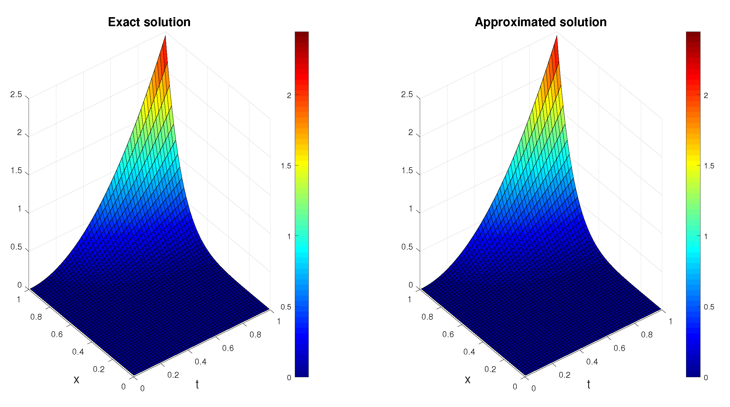
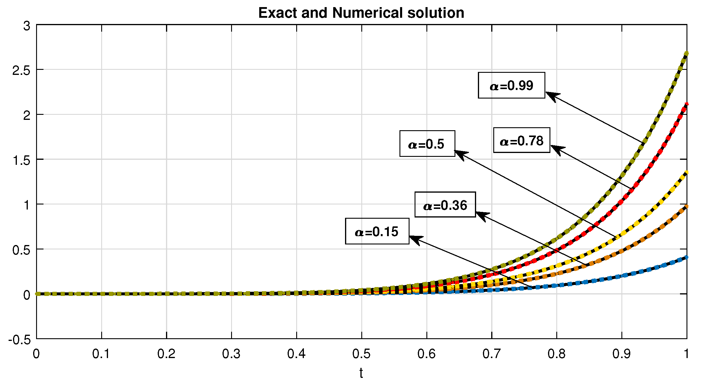
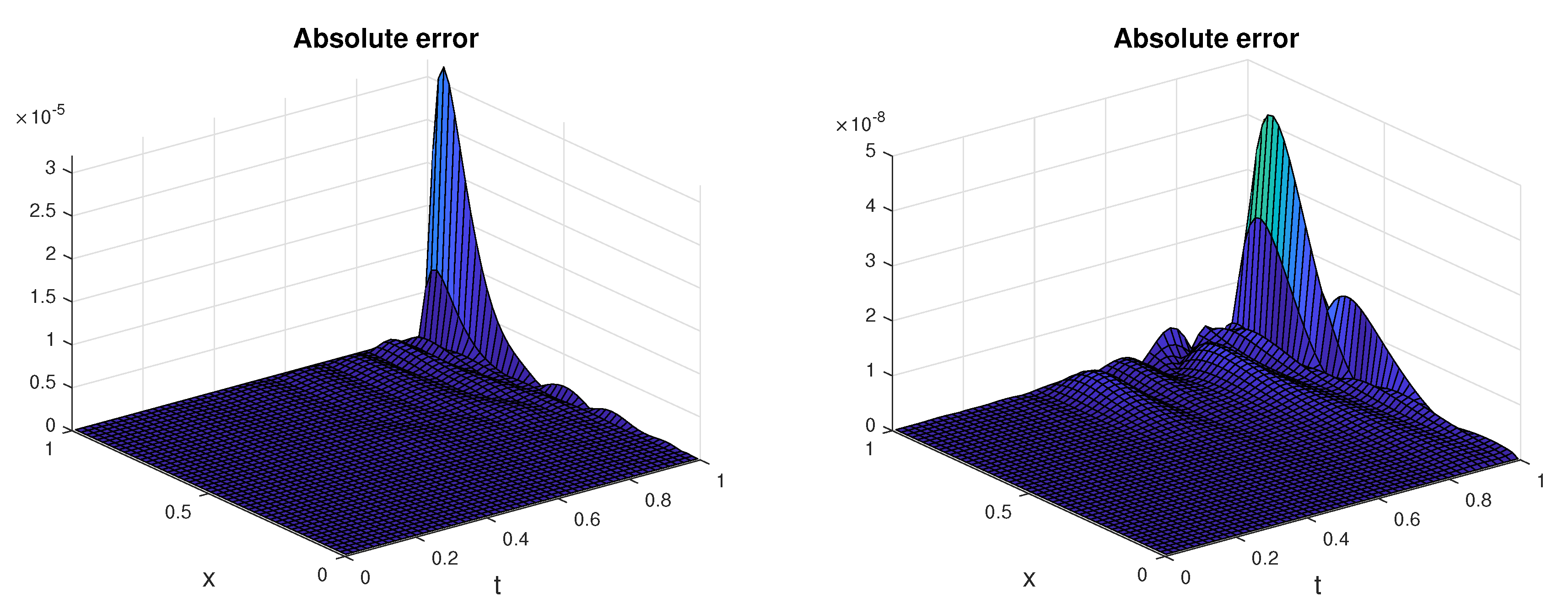
Now, we evaluate along discretized Brownian paths. To approximate , we use the discretized scheme described at the beginning of this section. Figure 1 displays the exact and approximate solution with and Figure 2 shows the exact solution and its estimations for different values of , when . These figures confirm that the resulted numerical solutions have good compatibility with the exact solution. Table 1 displays the -norm errors and convergence orders for and several values of N. Also, Figure 3 show the behaviour of the absolute error of for different values of N, when . Table 1 and Figure 3 confirm the accuracy of the obtained numerical approximations.
Example 2.
Suppose the time-fractional stochastic equation
where , is a Brownian motion, and
With these assumptions, the exact solution is .
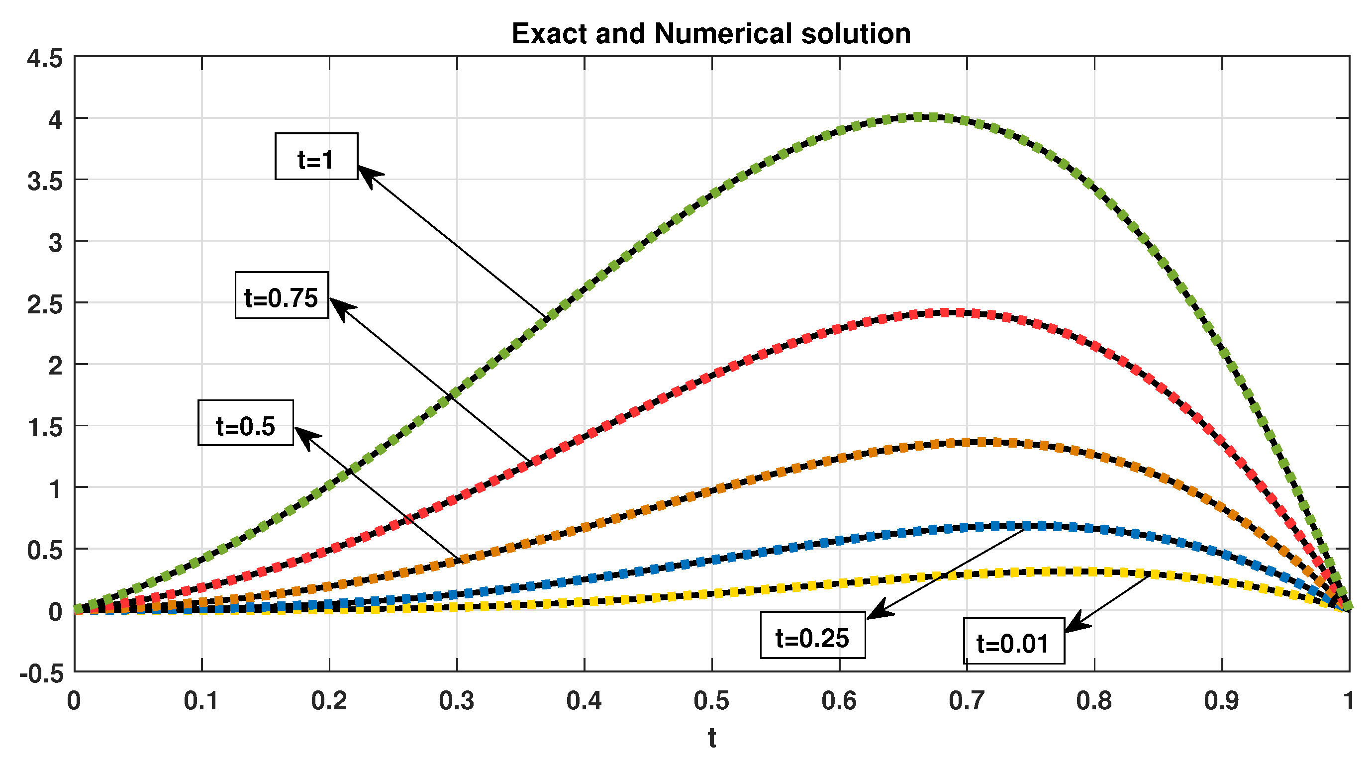
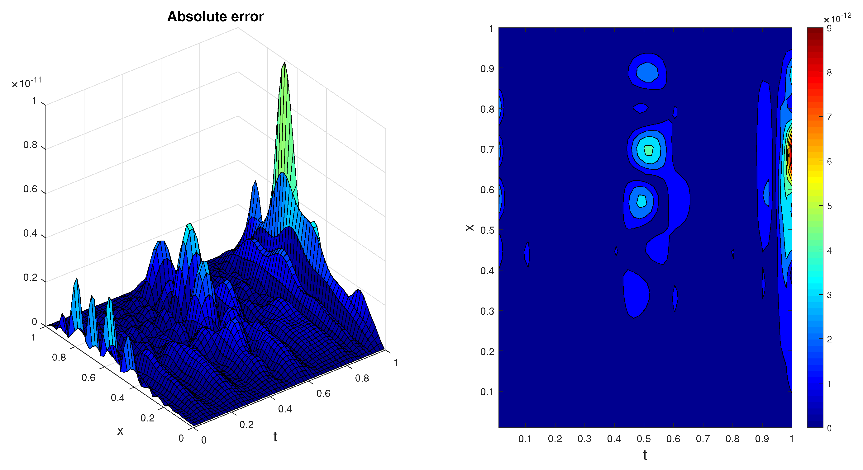
The numerical solution is evaluated along discretized Brownian paths. Table 2 displays the -norm errors and order of convergence for several values of and N. This table shows the high accuracy of the introduced scheme. Also, Figure 4 displays the exact and numerical solution of when , and Figure 5 indicates the absolute error together with the contour plot for . It can be seen that the numerical solution is in well agreement with the exact solution.
Example 3.
Let
subject to:
where and is a Brownian motion.
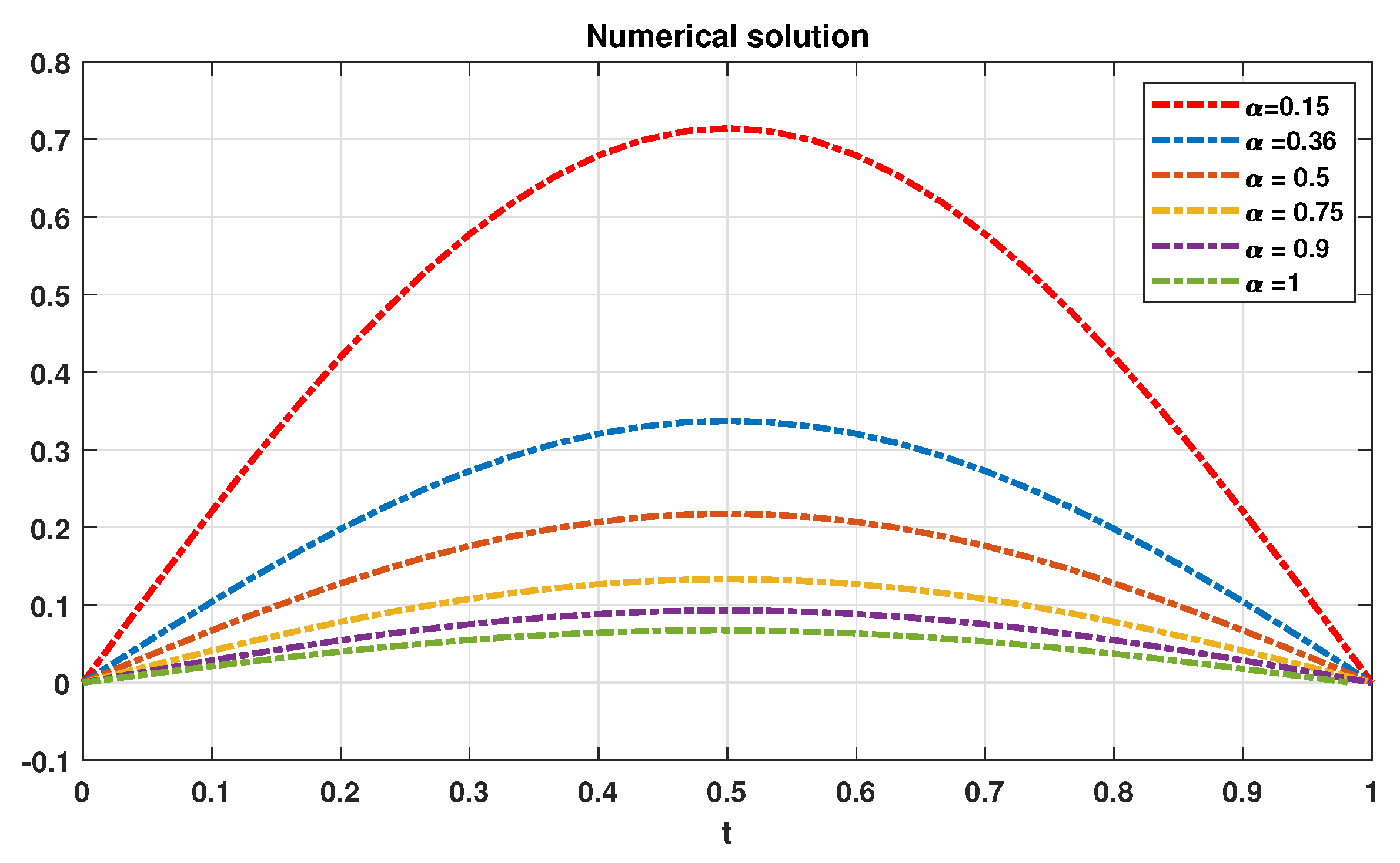
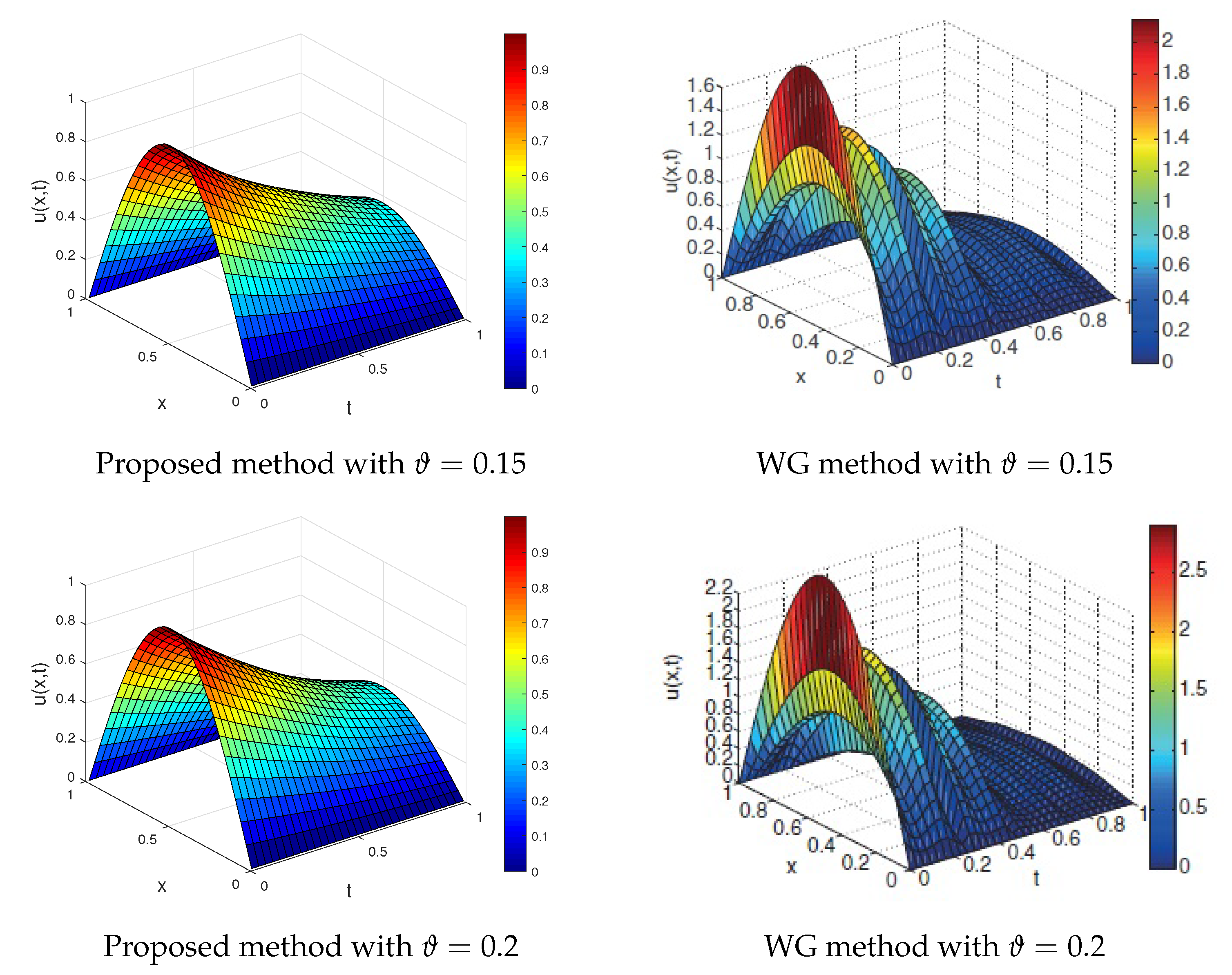
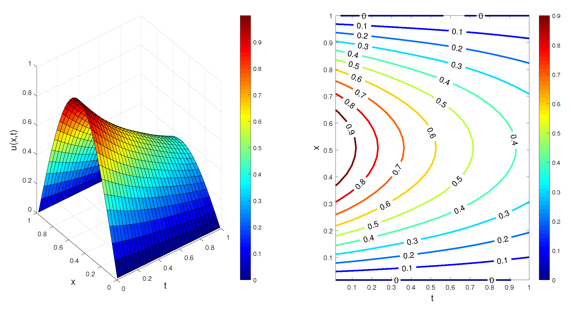
The numerical solutions are evaluated along discretized Brownian paths. Figure 6 shows the numerical solution at for different values of , when and . Figure 7 displays the estimation of when , and . The results are compared with wavelets Galerkin (WG) method [30]. This figure confirms that the present method gives more smooth solution than the numerical scheme in [30]. Also, Figure 8 and Figure 9 indicate the approximate solutions and the contour plots for several values of when . The results confirm that the employed approach is very efficient.
6. Conclusions
According to numerous applications of FSPDEs, a new numerical scheme was introduced to solve a class of stochastic heat equations of fractional order with additive noise subject to suitable conditions. This numerical method was based on a collocation approach with the SKCPs basis functions. The convergence of the proposed method was proved. Three illustrative examples were investigated to authenticate the efficiency of the discussed approach. The obtained numerical results approved the accuracy of this method.
Author Contributions
All authors discussed the results and contributed to the final manuscript. All authors have read and agreed to the published version of the manuscript.
Funding
This research received no external funding.
Conflicts of Interest
The authors declare no conflict of interest.
References
- Bellomo, N.; Brzezniak, Z.; Socio, L.M.D. Nonlinear Stochastic Evolution Problems in Applied Sciences; Kluwer Academic Publishers, Springer: Dordrecht, The Netherlands, 1992. [Google Scholar]
- Brace, A.; Gatarak, D.; Musiela, M. The market model of interest rate dynamics. Math. Financ. 1997, 7, 127–147. [Google Scholar] [CrossRef] [Green Version]
- Singh, S.; Ray, S.S. Numerical solutions of stochastic Fisher equation to study migration and population behavior in biological invasion. Int. J. Biomath. 2017, 10, 1750103. [Google Scholar] [CrossRef]
- Zmievskaya, G.I.; Bondareva, A.L.; Levchenko, T.V.; Maino, G. Computational stochastic model of ions implantation. AIP Conf. Proc. 2015, 1648, 230003. [Google Scholar]
- Chen, X.; Hu, P.; Shum, S.; Zhang, Y. Dynamic stochastic inventory management with reference price effects. Oper. Res. 2016, 64, 1529–1536. [Google Scholar] [CrossRef] [Green Version]
- Gillard, N.; Belin, E.; Chapeau-Blondeau, F. Stochastic antiresonance in qubit phase estimation with quantum thermal noise. Phys. Lett. A 2017, 381, 2621–2628. [Google Scholar] [CrossRef] [Green Version]
- Kilbas, A.A.; Srivastava, H.M.; Trujillo, J.J. Theory and Applications of Fractional Differential Equations; North-Holland Mathematics Studies; Elsevier: Amsterdam, The Netherlands, 2006; Volume 204. [Google Scholar]
- Podlubny, I. Fractional Differential Equations: An Introduction to Fractional Derivatives, Fractional Differential Equations, to Methods of Their Solution and Some of Their Applications; Academic Press: New York, NY, USA, 1999. [Google Scholar]
- Babaei, A.; Banihashemi, S. A stable numerical approach to solve a time-fractional inverse heat conduction problem. Iran J. Sci. Technol. Trans. A 2017, 42, 2225–2236. [Google Scholar] [CrossRef]
- Nemati, S.; Lima, P.M. Numerical solution of nonlinear fractional integro-differential equations with weakly singular kernels via a modification of hat functions. Appl. Math. Comput. 2018, 327, 79–92. [Google Scholar] [CrossRef]
- Babaei, A.; Banihashemi, S. Reconstructing unknown nonlinear boundary conditions in a time-fractional inverse reaction-diffusion-convection problem. Numer. Methods Part. Differ. Equ. 2018, 35, 976–992. [Google Scholar] [CrossRef]
- Tien, D.N. Fractional stochastic differential equations with applications to finance. J. Math. Anal. Appl. 2013, 397, 334–348. [Google Scholar] [CrossRef]
- Sabatelli, L.; Keating, S.; Dudley, J.; Richmond, P. Waiting time distributions in financial markets. Eur. Phys. J. B Condens. Matter Complex Syst. 2002, 27, 273–275. [Google Scholar] [CrossRef]
- Yu, Z.-G.; Anh, V.; Wang, Y.; Mao, D.; Wanliss, J. Modeling and simulation of the horizontal component of the geomagnetic field by fractional stochastic differential equations in conjunction with empirical mode decomposition. J. Geophys. Res. Space Phys. 2010, 115. [Google Scholar] [CrossRef]
- Schumer, R.; Benson, D.A.; Meerschaert, M.M.; Baeumer, B. Multiscaling fractional advection-dispersion equations and their solutions. Water Resour. Res. 2003, 39, 1022–1032. [Google Scholar] [CrossRef]
- Chaves, A.S. A fractional diffusion equation to describe Levy flights. Phys. Lett. A 1998, 239, 13–16. [Google Scholar] [CrossRef]
- Abdel-Rehim, E. From the Ehrenfest model to time-fractional stochastic processes. J. Comput. Appl. Math. 2009, 233, 197–207. [Google Scholar] [CrossRef] [Green Version]
- Chen, Z.Q.; Kim, K.H.; Kim, P. Fractional time stochastic partial differential equations. Stoch. Process. Appl. 2015, 125, 1470–1499. [Google Scholar] [CrossRef]
- Rajivganthi, C.; Muthukumar, P.; Priya, B.G. Successive approximation and optimal controls on fractional neutral stochastic differential equations with poisson jumps. Optim. Control Appl. Methods 2015, 37, 627–640. [Google Scholar] [CrossRef]
- Liu, W.; Tian, K.; Foondun, M. On some properties of a class of fractional stochastic heat equations. J. Theor. Probab. 2017, 30, 1310–1333. [Google Scholar] [CrossRef] [Green Version]
- Ralchenko, K.; Shevchenko, G. Existence and uniqueness of mild solution to fractional stochastic heat equation. arXiv 2018, arXiv:1811.12475. [Google Scholar] [CrossRef]
- Roozbahani, M.M.; Aminikhah, H.; Tahmasebi, M. Numerical solution of stochastic fractional pdes based on trigonometric wavelets. UPB Sci. Bull. Ser. A Appl. Math. Phys. 2018, 80, 161–174. [Google Scholar]
- Moghaddam, B.P.; Zhang, L.; Lopes, A.M.; Machado, J.A.T.; Mostaghim, Z.S. Sufficient conditions for existence and uniqueness of fractional stochastic delay differential equations. Int. J. Probab. Stoch. Process. 2019. [Google Scholar] [CrossRef]
- Mishura, Y.; Ralchenko, K.; Zili, M. On mild and weak solutions for stochastic heat equations with piecewise-constant conductivity. Stat. Probab. Lett. 2020, 159, 108682. [Google Scholar] [CrossRef]
- Gyongy, I.; Martinez, T. On numerical solution of stochastic partial differential equations of elliptic type. Stochastics 2006, 78, 213–231. [Google Scholar] [CrossRef]
- Roth, C. A Combination of Finite Difference and Wong-Zakai Methods for Hyperbolic Stochastic Partial Differential Equations. Stoch. Anal. Appl. 2006, 24, 221–240. [Google Scholar] [CrossRef]
- Walsh, J.B. On numerical solutions of the stochastic wave equation. Illinois J. Math. 2006, 50, 991–1018. [Google Scholar] [CrossRef]
- Du, Q.; Zhang, T. Numerical approximation of some linear stochastic partial differential equations driven by special additive noises. SIAM J. Numer. Anal. 2002, 40, 1421–1445. [Google Scholar] [CrossRef] [Green Version]
- Geissert, M.; Kovacs, M.; Larsson, S. Rate of weak convergence of the finite element method for the stochastic heat equation with additive noise. BIT 1995, 49, 343–356. [Google Scholar] [CrossRef]
- Heydari, M.H.; Hooshmandasl, M.R.; Loghmani, G.B.; Cattani, C. Wavelets Galerkin method for solving stochastic heat equation. Int. J. Comput. Math. 2016, 93, 1579–1596. [Google Scholar] [CrossRef]
- Moghaddam, B.P.; Zhang, L.; Lopes, A.M.; Machado, J.A.T.; Mostaghim, Z.S. Computational scheme for solving nonlinear fractional stochastic differential equations with delay. Stoch. Anal. Appl. 2019, 37, 893–908. [Google Scholar] [CrossRef]
- Mirzaee, F.; Alipour, S. Cubic B-spline approximation for linear stochastic integro-differential equation of fractional order. J. Comput. Appl. Math. 2020, 366, 112440. [Google Scholar] [CrossRef]
- Mirzaee, F.; Hadadiyan, E. Solving system of linear Stratonovich Volterra integral equations via modification of hat functions. Appl. Math. Comput. 2017, 293, 254–264. [Google Scholar] [CrossRef]
- Li, Q.; Kang, T.; Zhang, Q. Mean-square dissipative methods for stochastic age-dependent Capital system with fractional Brownian motion and jumps. Appl. Math. Comput. 2018, 339, 81–92. [Google Scholar] [CrossRef]
- Heydari, M.H.; Mahmoudi, M.R.; Shakiba, A.; Avazzadeh, Z. Chebyshev cardinal wavelets and their application in solving nonlinear stochastic differential equations with fractional Brownian motion. Commun. Nonlinear Sci. Numer. Simul. 2018, 64, 98–121. [Google Scholar] [CrossRef]
- Higham, D.J. An Algorithmic Introduction to Numerical Simulation of Stochastic Differential Equations. Soc. Ind. Appl. Math. 2001, 43, 525–546. [Google Scholar] [CrossRef]
- Liu, L.; Caraballo, T. Well-posedness and dynamics of a fractional stochastic integro-differential equation. Phys. D Nonlinear Phenom. 2017, 355, 45–57. [Google Scholar] [CrossRef]
- Darehmiraki, M. An efficient solution for stochastic fractional partial differential equations with additive noise by a meshless method. Int. J. Appl. Comput. Math. 2018, 4, 14. [Google Scholar] [CrossRef]
- Kovács, M.; Larsson, S.; Saedpanah, F. Mittag–Leffler Euler Integrator for a Stochastic Fractional Order Equation with Additive Noise. SIAM J. Numer. Anal. 2020, 58, 66–85. [Google Scholar] [CrossRef] [Green Version]
- Brzezniak, Z.; Debbi, L. On stochastic Burgers equation driven by a fractional Laplacian and space–time white noise, Stochastic differential equations: Theorem and applications. Interdiscip. Math. Sci. 2007, 2, 135–167. [Google Scholar]
- Shu, J.; Li, P.; Zhang, J.; Liao, O. Random attractors for the stochastic coupled fractional Ginzburg-Landau equation with additive noise. J. Math. Phys. 2015, 56, 102702. [Google Scholar] [CrossRef]
- Meerschaert, M.M.; Tadjeran, C. Finite difference approximations for fractional advection-dispersion flow equations. J. Comput. Appl. Math. 2004, 172, 65–77. [Google Scholar] [CrossRef] [Green Version]
- Masjed-Jamei, M. A basic class of symmetric orthogonal polynomials using the extended Sturm–Liouville theorem for symmetric functions. J. Math. Anal. Appl. 2007, 325, 753–775. [Google Scholar] [CrossRef] [Green Version]
- Babaei, A.; Jafari, H.; Banihashemi, S. Numerical solution of variable order fractional nonlinear quadratic integro-differential equations based on the sixth-kind Chebyshev collocation method. J. Comput. Appl. Math. 2020, 377, 112908. [Google Scholar] [CrossRef]
- Abd-Elhameed, W.M.; Youssri, Y.H. Sixth-kind Chebyshev spectral approach for solving fractional differential equations. J. Nonlinear Sci. Numer. Simul. 2019, 20, 191–203. [Google Scholar] [CrossRef]
- Jafari, H.; Babaei, A.; Banihashemi, S. A novel approach for solving an inverse reaction-diffusion-convection problem. J. Optim. Theory Appl. 2019, 183, 688–704. [Google Scholar] [CrossRef]
Figure 1.
The exact and numerical solution of Example 1 with .

Figure 2.
The exact and approximate solution for different values of in Example 1.

Figure 3.
The absolute errors for Example 1 when (left) and (right).

Figure 4.
The exact and numerical solution at different levels of t for Example 2.

Figure 5.
The absolute error (left) and contour plot (right) for Example 2 with .

Figure 6.
The numerical solution at for different values of in Example 3.

Figure 7.
The numerical solution obtained by the proposed method (left) and wavelets Galerkin method [30] (right) for Example 3 with different values of when .
Figure 7.
The numerical solution obtained by the proposed method (left) and wavelets Galerkin method [30] (right) for Example 3 with different values of when .

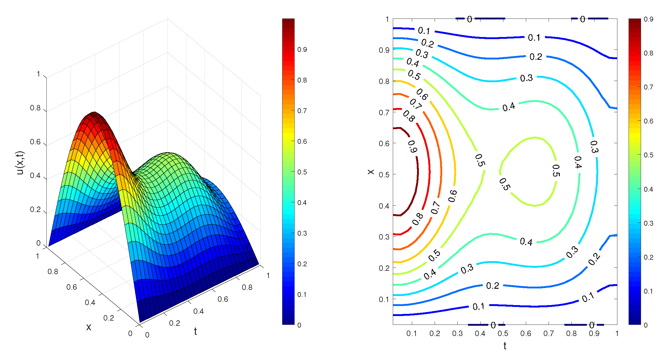
Figure 8.
The numerical approximation (left) and contour plot (right) for Example 3 with .

Figure 9.
The numerical approximation (left) and contour plot (right) for Example 3 with .


Table 1.
Example 1: The -norm errors and convergence orders.
| N | |||||
|---|---|---|---|---|---|
| CO | CO | ||||
| 6 | |||||
| 9 | |||||
| 12 | |||||
| 15 | |||||
Table 2.
Example 2: The -norm errors and convergence order.
| N | |||||
|---|---|---|---|---|---|
| CO | CO | ||||
| 6 | |||||
| 9 | |||||
| 12 | |||||
| 15 | |||||
© 2020 by the authors. Licensee MDPI, Basel, Switzerland. This article is an open access article distributed under the terms and conditions of the Creative Commons Attribution (CC BY) license (http://creativecommons.org/licenses/by/4.0/).
Share and Cite
MDPI and ACS Style
Babaei, A.; Jafari, H.; Banihashemi, S. A Collocation Approach for Solving Time-Fractional Stochastic Heat Equation Driven by an Additive Noise. Symmetry 2020, 12, 904. https://doi.org/10.3390/sym12060904
AMA Style
Babaei A, Jafari H, Banihashemi S. A Collocation Approach for Solving Time-Fractional Stochastic Heat Equation Driven by an Additive Noise. Symmetry. 2020; 12(6):904. https://doi.org/10.3390/sym12060904
Chicago/Turabian StyleBabaei, Afshin, Hossein Jafari, and S. Banihashemi. 2020. "A Collocation Approach for Solving Time-Fractional Stochastic Heat Equation Driven by an Additive Noise" Symmetry 12, no. 6: 904. https://doi.org/10.3390/sym12060904
Note that from the first issue of 2016, this journal uses article numbers instead of page numbers. See further details here.