The Fuzzy–AHP Synthesis Model for Energy Security Assessment of the Serbian Natural Gas Sector


Faculty of Mining and Geology, University of Belgrade, Djusina 7, 11000 Belgrade, Serbia
*
Author to whom correspondence should be addressed.
Symmetry 2020, 12(6), 908; https://doi.org/10.3390/sym12060908
Submission received: 20 April 2020
/
Revised: 13 May 2020
/
Accepted: 29 May 2020
/
Published: 1 June 2020
Abstract
:Natural gas is used for the production of almost 20% of total energy today. The natural gas security of the Republic of Serbia is an urgent strategic, political and security issue. Serbia is one of the most vulnerable countries in Southeast Europe, because it only has one supply route. This study is a contribution to efforts to better understand the factors affecting energy security through the implementation of a new methodology based on the fuzzy–AHP synthesis model for measuring energy security. This new methodology was used to identify the energy, economic, environmental, social and technical indicators that accompany energy security analysis. The fuzzy–AHP synthesis model uses the asymmetric fuzzy inference approach for an outcome finding with the asymmetric position of fuzzy sets. The most important characteristic of the proposed model is its ability to operate with numerical and linguistic data and universality of application. The result of the proposed model shows a quantified assessment of energy security and its trend in the future of the natural gas sector. It indicates an unacceptably low level of present energy security and a gas system very vulnerable to supply cuts if the current gas infrastructure remains as it is in the future.
1. Introduction
Energy is an essential ingredient for the world’s development. Energy represents a vital source of power for all social and economic activities and a unique part of the sustainable development puzzle. A key priority for almost all countries is the energy issue, the assurance of adequate energy supplies to sustain the country’s economy, new investments and market’s development [1].
The energy security is one of the most important parameters in determining the current position/condition and in defining the future development of all countries and regions. Demand for energy in the region of Southeast Europe is growing, but supply sources are increasingly limited and unevenly distributed. It is clear that the concept of energy security is becoming an important item for monitoring each country facing major energy changes [2]. Energy security, as a policy issue, became interesting in the early 1920s. It was directly connected with WWI and oil demand for the military [3]. Some years before and soon after the energy crisis in 1970s, energy security became an important field of academic research [4]. Although the academic interest in energy security declined with the stabilization of oil prices in the 1980s and 1990s, it became topical again in the 2000s because of the high demand in Asia, pressure to modernize and decarbonize energy systems and problems with gas supplies in Europe [5].
The definition of energy security has changed over the years. According to [5] there is division on contemporary and classic energy security studies. Back in the 1980s, energy security is was defined as the stable supply of cheap oil under threats of embargoes and price manipulations by exporters [6,7]. Contemporary energy security studies deal with security issues extending beyond oil supplies [8]. Today, energy security is closely connected with other energy problems, such as mitigating climate change and providing equal access to energy [9].
In general, energy security is inextricably linked to the national security of a country and as such can be considered in the context of comprehensive security, as well as an independent integral part of a more general term [10]. Energy security determines the continuous availability of energy in various forms, at affordable prices and in sufficient quantities [11].
Energy security is a parameter whose specificity lies in the influence of many factors, so it is not possible to define a unique methodology to determine [12]. Defining a methodological approach for determining the energy security of a country is possible only if the geopolitical moment, climatic conditions, wealth and availability of energy resources and their usage by type and intensity are taken into account. In addition, economic growth, demographic indicators, political priorities, market development, and energy scenarios have important roles [13,14,15,16]. Changing strategic priorities causes change in the methodology of energy security analysis, i.e., the methodology of measuring energy security is applicable only at a given moment [17].
1.1. Energy Security and Decision Making
Energy security from a decision-making perspective can be assessed by different approaches and models. According to [18,19,20], indicators are mainly proposed to measure different dimensions of energy security and to support decision-making. Methodologies are mainly reduced to the formation of an index that will express the degree of risk or level of security of an energy system [21]. Analysis of the current literature shows that the following methodologies are in active and most common use: Herfindahl–Hirschman index [22], S/D index [23], oil vulnerability index [24], import energy supply risk [25,26], techno-economic-social risk [27], index of us energy security risk [28], MOSES—IEA model of short-term review of energy security [29], energy security index developed by the EU Center for Joint Research in Italy [30] and the global energy architecture performance index, proposed by the World Economy forum [31].
Multi-criteria analyses are another tool used to support decision-making [32,33,34]. These kinds of models can be used to analyze both qualitative and quantitative aspects of energy security. Some of the models for energy security assessment have originated from different scientific backgrounds. For example, the POLES-model, top-down economic model, operates with economic and demographic development as input parameters, to assess supply and demand of energy up until 2050 [35]. ERIS is a multi-regional bottom-up optimization model with technology learning that researches global trends in supply up until 2100 [36]. According to [37] there is also a combination of these different models. Based on [34], it was proposed that the use of an analytical process of hierarchy by which experts compare different aspects, policies or scenarios and rank them individually according to their assessment and a set of predefined criteria. Various methods of multi-criteria analyses have so far been used to assess energy development scenarios: AHP (analytical hierarchy process), MAUT (multi-attribute utility theory), SMART (simple multi-attribute ranking technique) are just some of them [38]. Specialized methods such as AMS (combination of the previous three) have been created for the purpose of assessing the impact of climate change policy and relevant policy measures, because in addition to assessing different energy development scenarios, it also provides assessments on climate change mitigation policy and climate change adaptation, with the possibility of assessing their mutual interaction [38].
Multi-criteria decision-making (MCDM) methods integrated with fuzzy set theory have been widely used to deal with uncertainty in the energy field decision process [39,40,41]. The key reason is finding an appropriate language to manage imprecise criteria and the possibility of integrating the analysis of qualitative and quantitative factors.
1.2. Energy Security and Fuzzy Theory
Fuzzy theory finds its purpose in the analysis and modeling of complex systems, starting from the idea that complex problems can be solved if instead of rigor and greater accuracy of descriptions of certain phenomena, the exact opposite is done, making those descriptions imprecise [42]. In classical (bivalent) logic, each statement can only be true or false, that is, the value of a statement can be only 0 if the statement is false and 1 if it is true. There are many statements in human speech that do not have a strictly true/strictly false value. Fuzzy theory represents the concept of the value of truth that ranges from the notion of completely true to the notion of completely false (0–1) [43]. Fuzzy logic, as well as the accompanying theory of fuzzy sets, is tolerant of imprecise data and flexible in the field of application, thus representing an intuitive feature of human reasoning [44]. In addition, the fuzzy set theory reduces the influence of analysts to a minimum, at the same time representing part of artificial intelligence which is not a feature of multi criteria methods. In addition, the fuzzy set theory has more efficient operational power with hybrid data and we get the surface as a final result. This is especially important, because the key characteristics of such a result are the ability to see the center of gravity, dispersion of results and tendency (“time state picture”). Models based on fuzzy set theory are not just decision-making, but also optimizing.
The proposed research in this article tries to prove the possibility of using the theory of fuzzy sets proposed by Zadeh [42] to describe indicators of energy development scenarios. Energy development indicators are usually relative or absolute numerical values that link the parameters of energy development with economic, environmental, social and other parameters related to that development (energy consumption/production per capita, per unit of gross domestic product, by amount of emitted pollutants, etc.). However, some of the important indicators that describe energy development, such as security of supply, energy security, competitiveness of the economy, political acceptability, etc., are not so simple to quantify because there is no conventional way of defining, evaluating and measuring them. Fuzzy sets theory has attracted widespread attention in various fields, especially where conventional mathematical techniques are of limited effectiveness. By using fuzzy set for the description of indicators, on one hand, a unified description will be obtained, which, on the other hand, will carry all the benefits of their linguistic description.
Despite the inability to find a common methodology, the framework in which the process of analysis and assessment of energy security takes place is still uniform. In practice, the improvement of energy security is accompanied by the implementation of energy efficiency measures, raising the level of stability and liquidity of energy entities and the system, increasing the level of self-sufficiency and reducing the level of vulnerability (strengthening the market, renovating and improving the system, raising storage capacities, intensifying research for new sites and raising use of modern technology of exploitation, etc.) [45,46]. The aim of this study was to investigate the energy security of the potential development of natural gas sector in Serbia, and to create a model that comprehensively analyzes energy security even from the aspect of partial indicators that are not so simple to quantify and in the end to develop a methodology that can quantify energy security. The methodology proposed in this article is based on fuzzy set theory and AHP ranking and integrally considers the level of quality and intensity of scenarios from energy, economic, environmental and social views. The process of compositing fuzzy relationships was done using a “max–min” model of fuzzy composition. One of the key characteristics of the proposed methodology was its attempt to adopt the group of synthetic indicators that are commonly used in earlier multi-criteria mathematical models. The reason for referring to already traditional methods is the desire to compare the results of the model developed with these mentioned traditional mathematical models. The initial idea for this study was to create a model that comprehensively analyses energy security even from the aspects of the partial indicators that are not so simple to quantify.
The study is divided into seven sections. Section 1 comprises an introduction about energy security and different approach of analysis and assessment of energy security; Section 2 explains the rationale and the principles for modeling energy security with the fuzzy–AHP synthesis model for analysis energy security of the gas sector. This section provides analysis of basic steps of methodology and key elements that are involved in model; Section 3 provide information about the current state of the natural gas sector of the Republic of Serbia and infrastructure development plan; Section 4 demonstrates the application of the proposed methodology for the evaluation of the energy security assessment for the natural gas sector in Serbia; Section 5 is reserved for results of the case study; Section 6 provides discussions; and finally Section 7 draws conclusions.
2. The Fuzzy–AHP Synthesis Model for Energy Development Scenarios
During the procedure, data collection is performed, which can be statistical (based on calculation, software model result, projections, statistical processing, etc.) or based on expert analysis, i.e., attitude and experts. After that, the data are classified and entered in an adequate form into the model of integral analysis. Such data are entered into the synthesis model by the fuzzy proposition procedure, where in the further process of fuzzification data are defined as input data to the fuzzy set. Ranking is performed at the same time. It can be performed by a number of different methods and for the purposes of developing this synthetic model; ranking based on the application of the multi criteria AHP (analytic hierarchy process) method was used. In this way, the ranking data are used as input data to the fuzzy set, which is further analyzed in the fuzzy composition process. Fuzzy compositions represent a step in modeling using fuzzy set theory in which the process of integration and synthesis of partial influences at the synthetic level is performed. The process of compositing fuzzy relationships can be performed in a variety of ways. Several models of fuzzy composition are mentioned in the literature and the following are the most commonly used.
- Max–min composition is one of the intensively used fuzzy composition models. It is also called a pessimistic composition due to the procedure by which it is performed—the presentation of a synthetic grade using a representative partial grade, which is defined as the best possible among the worst expected individual grades [48,49];
For phenomena that carry potential negative connotations (risk, safety, etc.), the max–min composition is considered better [50]. According to [51], based on mathematical analysis, it has been proven that the composition max–min performs a more precise grouping of results and the mutual establishment of relations between results is more pronounced. In other words, the mentioned composition prevents unnecessary dissipation of results and contributes to additional precision and a realistic foundation for the final grade. Specifically, for energy security, the max–min concept will yield the best possible results among the worst outcomes, thus leading to a relatively high grade through the marginalization of estimation errors [52].
As a result of the fuzzy composition, an energy security assessment is made. The output data of the fuzzy set is defuzzificated throughout the identification procedure. The “best-fit” and “gravity center“ methods are used to identify the output data from the fuzzy composition. Using these methods, the assessment of energy security is expressed depending on the function of affiliation and class, i.e., depending on linguistic variables.
Linguistic variables (LV) are those variables whose values are actually the word or words of natural language as the basis of human communication. Linguistic variables always consist of basic linguistic values. By adding linguistic modifiers (less, more, very, very much, etc.), as well as conjunctions (and, or, not), complex linguistic expressions can be obtained. Linguistic variables can be assigned one or more linguistic values that are related to numerical values through membership and class functions [48]. For example, if the variable “STRENGTH” can have the values weak, strong, very strong, not weak, very weak, etc., then STRENGTH is a linguistic variable. Words strong, weak, not weak, etc. are values of linguistic variable or linguistic value. In that case, linguistic modifiers are very, many, etc.
The fuzzy–AHP synthesis model for evaluation of energy security assessment of energy development scenarios is explained in detail in this section.
2.1. Indicator Structure
An integral analysis of the energy security of the natural gas sector of the Republic of Serbia was carried out by developing a mathematical model that considered a group of synthesis and partial indicators that are very specific for the given political, strategic and energy momentum. The fuzzy–AHP synthesis model for integral analysis of energy security with modified outcome through ranking was proposed. The indicator structure is shown in Figure 1, and it is used to define the level of energy security in the two stages of the analysis, for a certain energy scenario. The indicator structure is thus created to be an operational, decoupling, but also complete entity, without excessive detail, minimized to the extreme level [53]. Indicators are independently, measurable and comprehensive [54].
For the purpose of model creation, a group of three synthesis indicators was analyzed, which were more precisely defined using three partial indicators. Analyzing the earlier common use of multi-criteria mathematical models for the analysis of energy development scenarios, the following group of synthesis indicators was adopted: socioeconomic applicability (A), security of supply (S) and environmental acceptability (E).
The fuzzy–AHP synthesis model is structurally and hierarchically composed of two steps.
The first level of synthesis is related to the composition of:
- Administrative applicability (A1), economic feasibility (A2) and affordability (A3) to socioeconomic applicability (A);
- Availability of energy (S1), diversification of sources and routes (S2) and infrastructure development (S3) into security of supply (S);
- GHG emission (E1), pollutant emission (E2) and the indirect environment effect (E3) into environmental acceptability (E).
The second level of synthesis is related to the composition of:
- Socioeconomic applicability (A), security of supply (S) and environmental acceptability (E) into energy security (ES).
Socioeconomic applicability is a synthesis indicator described through the attitude of all relevant entities involved in the process of implementing activities related to the acceptability and economy of a scenario. It is directly linked to national structures (institutions and human resources) [36], as well as the legal framework that follows relevant issues.
The security of supply is a synthesis indicator that can be viewed in a very broad context. It is generally defined using a set of sub-indicators, such as: availability of energy, accessibility, acceptability, security and political stability [55,56]. However, for the development of a methodology that will analyze the scenarios of the development of the natural gas sector, the security of supply indicator focuses primarily on specific partial indicators that deflect the definition of supply stability, the number and types of interconnections and sources of natural gas and the development of the gas pipeline network in the Republic of Serbia.
Environmental acceptability expresses the total contribution of the observed activity to a state of the environment, which may be indicated by a set of partial indicators. Some of them, such as emissions of greenhouse gases and/or pollutants, are directly measurable, while others represent the accompanying results of the act or emission within the analyzed scenarios of energy development. This partial indicators greenhouse gases (GHG and pollutants emission and indirect environment effect) shows the reduction or increase of emissions at the national, but also at the sectorial level, the proportion of the use of renewable sources, as well as the energy intensity by sectors, the reduction in energy use (total or sectorial) [36]. Table 1 shows partial indicators description and quantification.
The methodology of analysis of energy scenarios is shown in the next subsection.
2.2. Methodology Steps
The methodology of the analysis of the energy scenarios consisted of several basic steps in which it were realized. Figure 2 shows schematic diagram of basic methodology steps.
(I) The first step in the formation of the synthesis model was the proposition of partial and synthesis indicators (P1, P2, P3 and M). Five linguistic variables were introduced for each indicator, which were defined in the coordinate system of membership function (µ) and class as representative of the unit of measure of indicator (j). A linguistic variable (LV) was generally defined as follows:
LV = (µ(j = 1), …, µ(j = 10))
The linguistic variables were specifically defined as follows (Figure 3):
A = (0(1), …, 0(8), 1(9), 1(10));
B = (0(1), …, 0(5), 0.33(6), 1(7), 1(8), 0(9), 0(10));
C = (0(1), 0(2), 0(3), 0.5(4), 1(5), 1(6), 0.5(7), 1(8), 0(9), 0(10));
D = (0(1), 0(2), 1(3), 1(4), 0.33(5), 0(6), …, 0(10));
E = (1(1), 1(2), 0(3), …, 0(10)).
B = (0(1), …, 0(5), 0.33(6), 1(7), 1(8), 0(9), 0(10));
C = (0(1), 0(2), 0(3), 0.5(4), 1(5), 1(6), 0.5(7), 1(8), 0(9), 0(10));
D = (0(1), 0(2), 1(3), 1(4), 0.33(5), 0(6), …, 0(10));
E = (1(1), 1(2), 0(3), …, 0(10)).
The use of the trapezoidal shape in defining the fuzzy set membership was expressed in linguistic variables where there was no clear and precise difference in the fuzzy conditions, while the function of the triangle shape affiliation was with much more precise linguistic variables [59]. Asymmetric fuzzy sets, inference and layout had been used in fuzzy synthesis model. It was obvious that there was a possibility for deviation in the behavior of the observed energy security. Those provoked needs for asymmetry in some shapes that defining the fuzzy set memberships. This definition of linguistic variables did not apply only in the case of the synthesis indicator security of supply (S) and the partial indicator availability of energy (S1). They were characterized by greater security of determining a more precise position in the coordinate system of membership functions. The linguistic variables in this case were specifically defined as follows (Figure 4):
A = (0(1), …, 0(8), 1(9), 0(10));
B = (0(1), …, 0(6), 1(7), 1(8), 0(9), 0(10));
C = (0(1), 0(2), 0(3), 0(4), 1(5), 1(6), 0(7), 1(8), 0(9), 0(10));
D = (0(1), 0(2), 1(3), 1(4), 0(5), …, 0(10));
E = (0(1), 1(2), 0(3), …, 0(10)).
B = (0(1), …, 0(6), 1(7), 1(8), 0(9), 0(10));
C = (0(1), 0(2), 0(3), 0(4), 1(5), 1(6), 0(7), 1(8), 0(9), 0(10));
D = (0(1), 0(2), 1(3), 1(4), 0(5), …, 0(10));
E = (0(1), 1(2), 0(3), …, 0(10)).
(II) The second step in the formation of the synthesis model was the fuzzification of the input data.
(IIa) In the case of expert evaluations, questionnaires were formed in which the answers of the corresponding linguistic variable with the given descriptions were offered. The role of the questionnaire was to had a set of statements, opinions and views of multiple participants competent to provide answers to specific questions asked, to sublimate in one place and to provide results that can be analyzed.
Questionnaires were prepared for the purpose of analyzing the partial indicators of administrative applicability (A1) and indirect environmental effect (E3) to conduct expert evaluation. Analysts whose area of business interest is closely related to the energy sector of the Republic of Serbia were interviewed. The questionnaire contained the possibility to choose one of several linguistic values of a particular linguistic variable with a detailed description of the meaning of each. In this way, analysts were able to express their opinion on the affiliation of the observed partial indicator to a specific variable (one entirely or more of them in a given proportion). The total score for the indicator mentioned above should have been 1 or 100%.
The questionnaire was drafted so that it was accompanied by a specific description of the grade, i.e., linguistic variables that describe a particular attitude. This is also a recommendation for how to complete the questionnaire itself. The results of the questionnaire were generated by processing the collected data with the classical mathematical methods of the law of statistics.
(IIb) In the case of numerically input data, mapping of class j size with real values of the observed phenomenon was performed. Theoretical value of a particular partial indicator (economic feasibility (A2), affordability (A3), availability of energy (S1), diversification of sources and routes (S2), infrastructure development (S3), GHG emission (E1) and pollutant emission (E2)) can be determined by the used of certain formulas. The actual value can be determined either by direct measurement or by numerically expressing the specific conditions under which partial indicators were observed. Large discrepancies between these values indicate the problems described through the partial indicator for a particular scenario. In contrast, small deviations will indicate good estimates of the partial indicator. The functional fuzzy number of a particular partial indicator for the observed scenario was defined using the average deviation between the real and theoretical values. The value for the class as representative of the unit of measure of the indicator (j) was defined taking into account the lowest recorded deviation (j = 10) and the largest recorded deviation (j = 1).
(III) Ranking was done in a third step. There are a number of ranking methods in the literature. The analytic hierarchy process (AHP) method was used in this study. AHP is a mathematical method in multi-criteria decision-making (MCDM) that is most often used [60]. This method is characterized by the possibility to emphasize the influence of a partial indicator in the description of the synthesis indicator and to minimize the subjective influence of the model’s author. The multi-criteria AHP method uses the Satie scale of parameter significance assessment [61]. AHP matrix consists of relative weights and its calculation provides outcome ranking. The estimate of relative weights shall be expressed as follows:
for i,j = 1, …, n.
aij= aij/Σaij
The criteria weight is then determined using the form:
for i,j = 1, …, n.
wi= aij/(n·Σaij)
The consistency check is expressed as follows:
bi = wi∙the parameter element within the matrix
Then the eigenvalue of the matrix is calculated using the expression:
and the weighted mean of coefficient λi:
λ = wi/bi
λmax = 1/n∙∑λi
As the last stage of the AHP upgrade to the modeling stage, a consistency check is performed by finding the consistency index CI,
which is further used to define the random consistency index CR:
where:
CI = (λmax − n)/(n − 1)
CR = CI/RI
RI—empirical consistency index of the multi-criteria AHP method (for n = 3, RI = 0.58 [62]).
The aforementioned ranking procedure using the AHP method was repeated for each partial indicator within each synthesis indicator.
(IV) The fourth step in the formation of a synthesis model was the composition of partial indicators to the level of synthesis. The composition was the final step in developing the methodology for the fuzzy–AHP synthesis model analysis. When assessing the energy security level of a particular energy development scenario, it was necessary to link all the impacts of the partial indicators. The synthesis was performed using the appropriate fuzzy composition. Several models of composition were mentioned in the literature. For phenomena that carry potential negative connotations (risk, safety, etc.), the max–min composition was better considered [50]. According to [51], it has been proven that the max–min composition performs a more precise grouping of results and expresses the mutual establishment of relations between results. Max–min composition prevents unnecessary waste of results and contributes to the additional precision and realistic justification of the final outcome [52]. For energy security, the max–min concept will produce results that will be the best possible among the worst outcomes, thus leading to a relatively high score through the marginalization of estimation errors [63,64].
The fuzzy asymmetric max–min composition model (steps 1–8) will be shown below [65].
Мi = max{min(P1i, P2i, P3i)}
- Three fuzzy numbers P1i, P2i and P3i are defined by the membership function μ and class j = 1 to n:P1i = (μP1(1), …, μP1(j), …, μP1(n));
P2i = (μP2(1), …, μP2(j), …, μP2(n));
P3i = (μP3(1), …, μP3(j), …, μP3(n)) - Affiliation functions can form C = n3 combinations with each other. Each combination represents practically one possible assessment Mi.for every c = 1 to C.Mc = [μP1(j=1, …, n), μP1(j=1, …, n), μP1(j=1, …, n)],
- If only the values that satisfying the condition µPi (j = 1, ..., n) ≠ 0 are taken into account, then the outcome is obtained o (o = 1 to O, where O ≤ C). Each outcome has corresponding values (iv) and (v) that further identify it for the calculation.
- In the following, for each combination c which satisfies the condition of outcome, the value of Jc is calculated and rounded as integer, as follows:wherе:Jc = (kP1i · j(μP1)c) + (kP2i · j(μP2)c) + (kP3i · j(μP3)c)
- -
- ki is the influential factor of the corresponding partial indicator on the synthesis and obtained on the basis of mutual ranking of the partial indicators (step III), where: kP1i + kP2i + kP3i = 1;
- -
- jc is the class to which the corresponding fuzzy number (3) belongs for the observed membership function and the given combination c, where: jc = 1, ..., n;
- For each outcome, a minimum value of μP1,P2,P3 in the vector Mc (4) is required, as follows:for every o = 1 дo O.MINo = min{μP1(j)o, μP2(j)o, μP3(j)o},
- The outcomes are grouped according to the knowledge of Jc. The number of such groups can be 0 to n.for every j = o.MAXj = max{MN1, …, MNo, …, MNO}Jc,
- The assessment M of the observed system is finally obtained in the form that agrees with its expressions with (1) and (12):M = (MAXj=1, …, MAXj=n) = (μM(1), …, μM(j), …, μM(n))
(V) Using expression 17, the assessment was obtained depending on the affiliation function and class. Using one of the fuzzification and identification methods, the assessment of energy security (M) can be expressed depending on the linguistic variables A, B, C, D, E according to Figure 5 and expression 2. In defuzzification process it is necessary to identify, which maps the energy security assessment of a particular energy development scenario to the fuzzy set of the ES indicator. For the purposes of this study, a best-fit method will be used. It was used to transform an energy security (M) assessment into a form that defines the degree of belonging of an energy security assessment to a particular fuzzy set or linguistic variable—very low, low, moderate, high and exceptional [66]:
for k = 1, …, 10, where LVi = {very low, low, moderate, high and exceptional} is defined with expression 1 and 2.
di(Mi, LVi) = SQRT(ΣμMk − αLVik)
The ‘best-fit’ method uses the distance di between the energy safety assessments M of the observed system defined through the asymmetric max–min composition of expression 17 and the linguistic variables A, B, C, D, E shown in Figure 5 and defined by expression 2. The distance di is used to show the degree of affiliation of an energy security assessment to a particular fuzzy set.
The closer the value of the energy security assessment is to the linguistic variable, the smaller the distance is. This distance is equal to 0 if the energy security estimate is the same as the ith expression in terms of belonging to the fuzzy set. In this case, the exclusivity of affiliation should not be further considered.
If we introduce that α1 to α10 are the reciprocal values of relative distances that are calculated as the ratio between the corresponding values of distances di and the values of dimin (i = 1, …, 10) which is at least among the distances obtained for M. Then αi can be expressed as:
αi = 1/(di/dimin)
If di = 0, then αi = 1, while the other reciprocal values of relative distances are then 0. In this case, αi is normalized:
Each βi represents the degree to which the energy security assessment (M) belongs to i-defined energy security terms. If Mi belongs entirely to the ith expression, then βi = 1 and the others are 0. Normalized βi can be seen as the degree of confidence that Mi belongs to that linguistic expression of energy security. The final expression of identified energy security performance is:
Mi = {(βi = 1, “very low”), (βi = 2, “low”), (βi = 3, “modern”), (βi = 4, “high”), (βi = 5, “exceptional”)}
In another defuzzification procedure, the quantitative assessment of energy security is the subject of the last step procedure in which the center of gravity is found as a number in the range from 0 to 10. This number speaks of the energy security itself, such that the increase in the center of gravity value represents a higher level of ES. The value of the center of gravity T is mathematically expressed as:
T = Σ(μM1, …, μM10)/Σ(μM1/1, …, μM10/10)
After establishing all five steps, a clear assessment of the energy security of a particular energy development scenario could be defined. This procedure provided a numerical solution for expressing a quantitative assessment of energy security, which is the ultimate goal of the fuzzy–AHP synthesis method. This established the measurability and comparability of the concept of energy security within different energy development scenarios.
3. Natural Gas Sector in Serbia
This section summaries basic information about current state and future developments plans for the natural gas sector in the Republic of Serbia.
3.1. Current State
Natural gas has been produced in Serbia since 1951. The Oil industry company of Serbia—NIS was owned by the state and obligated for gas production. In 1991, NIS becomes a vertically integrated Energy Company. Its role was to explore, produce, refine and trade crude oil and their derivate and natural gas [67]. In 1979, maximum production was achieved (1.14 billion m3). Since then, production was in steady decline until 2008 (3% increase compared to 2007). Average indigenous production was approximately 600 million m3 in the 1970s and the 1980s, and it has never achieved 20% of total consumption [68]. The Company NIS becomes NIS Gazprom Neft after change of ownership in 2009. It introduced a new business course and investment in modern technology [67]. This was defined based on the Agreement of the Republic of Serbia and the Government of the Russian Federation on Cooperation in the Oil and Gas Industry concluded in January 2008 and signed in October 2009 [69]. This reflected on intensive indigenous production (around 480 million in 2012). Natural gas production in the last 8 years is shown in Table 2. The main gas fields are in Vojvodina, the Serbian part of the Pannonia Basin. All gas fields relate to consumers with pipeline network. The capacity of these fields is enough to meet approximately 20% of the current needs of the Republic of Serbia for natural gas [70]. With the domestic production of 335 million m3 in 2018, only 13.5% of needs could be met [71].
The main pipeline system in Serbia starts from an interconnection with Hungary which allows gas imports from Russia and gas transit to Bosnia and Herzegovina (Figure 5). The natural gas transmission is performed by two transmission system operators, PC Srbijagas, Novi Sad and joint stock company Yugorosgaz-Transport LLC, Niš. Natural gas distribution and distribution system operation are performed by 32 licensed distribution system operators. Most of them are owned by municipalities and towns, some of them are public-private partnership, and some of them are private companies [71].
The current transmission system has the capacity to transport around 6 billion m3 of natural gas per year. Technically, with available interconnector capacity for natural gas customers in Serbia of 11 million m3/day and an interconnector utilization rate of 90%, it is possible to have around 3.6 billion m3/year of natural gas imported [68]. In 2018, the highest daily quantity import into the transmission system on the Serbian-Hungarian border was 11.39 million m3–9.66 million m3/day was used by customers in Serbia, while 1.73 million m3/day were intended for Bosnia and Herzegovina [71]. The average annual import in the ten-year period 2008–2018 was 1.093 billion m3, while 2.204 billion m3 of natural gas was imported in 2018 [71]. Table 3 shows transmitted natural gas quantities from all sources in the last five years.
There is one facility storage for natural gas, Underground Storage Banatski Dvor, which performs natural gas storage and storage operation. It is founded and owned by PC Srbijagas (49%) and Gazprom Germania (51%) [67]. The very first underground gas storage “Banatski Dvor” was finalized and operational in 2011. It is located on a depleted gas deposit whose capacity used to amount to 3.3 billion m3 of natural gas. Current available capacity is 450 million m3. The designed withdrawal daily capacity quantities are 5 million m3. The second development phase is planned and the storage will have the capacity of 800 million m3 [71]. In 2018, maximum daily injection quantities 2.6 million m3/day was recorded, and maximum daily withdrawn quantities was 4.99 million m3 [71]. The main characteristics of natural gas infrastructure in Serbia are shown in Table 4.
3.2. Natural Gas Development Plan
Six possible future projections in natural gas sector in Serbia by 2030 were created as a combination of infrastructure and consumption scenarios. The result of this model would provide quantification of energy security for various futures considering different supply options as well as different requirements of natural gas.
3.2.1. Scenarios of infrastructure development
Diversification of sources and directions of the natural gas supply, with establishing a domestic and regional natural gas market and providing the secure supply of natural gas are important goals in the natural gas sector of Republic of Serbia [2]. In 2017, Serbia adopted a Program for the Implementation of the Energy Development Strategy of the Republic of Serbia [58].
This Program presents a list of main infrastructure projects:
- Gas interconnection project with Bulgaria—main gas pipeline MG-10 Niš (Serbia)—Dimitrovgrad (border with Bulgaria) with 109 km length (in Serbia) and a planned capacity of 1.8 BCM per year with investment costs of 85.5 million € [58];
- Gas interconnection project with Croatia—main gas pipeline MG-08 Gospodjince (Futog, Serbia)—Sotin (border with Croatia) with 95 km length (in Serbia) and a planned capacity of 1.5 BCM per year with investment costs of 60 million € [58];
- Gas interconnection project with Romania—main gas pipeline MG Mokrin (Serbia)—Arad (border with Romania) with 6 km length (in Serbia) and a planned capacity of 1.6 BCM per year with investment costs of 85 million € (6 million € part of investment in Serbia) [58];
- Expending Underground storage “Banatski Dvor” capacities from 800 mcm to 1 BCM per year with investment costs of 65 million € [58].
Based on this list of infrastructure projects three different scenarios for natural gas infrastructure development were created for further analysis. These scenarios were also created with the possibility of providing investments. The characteristic scenarios of infrastructure development are:
- Business as Usual scenario (BAU) which is based on infrastructure development of the gas sector in accordance with key projects in strategic documents [58]. This scenario provides existing interconnection with Hungry (capacity 11 mcm per day) and a new one with Bulgaria with capacity of 4.93 mcm per day [2], and a possible connection to Turkish Stream (supply from Russia) and TAP (supply from Azerbaijan). The capacity of the “Banatski Dvor” underground storage is increased to 800 mcm and UGS capacity would be 9.96 mcm per day [2,58].;
- The most optimistic scenario of natural gas infrastructure development (OPT) is characterized with two additional supply interconnections comparable to BAU and increased capacities of additional UGSs to 1 BCM. This scenario is in line with the goals of the Energy Community in the SEE region [73] and it brings out existing interconnection with Hungry (capacity 11 mcm per day) and a new one with Bulgaria with capacity of 4.93 mcm per day, Romania with capacity of 4.38 mcm per day and Croatia with capacity of 4.1 mcm per day and new route of supply from Algeria through Italy [2,58].
3.2.2. Scenarios of Natural Gas Consumption
The Energy Development Strategy of the Republic of Serbia envisages different projections of consumption in the natural gas sector through different scenarios following various assumptions (level of implementation of energy efficiency measures, level of gas penetration for electricity generation, real GDP growth, etc.). Based on these predictions, two scenarios of natural gas consumption were formed for the purposes of this study (Table 5):
- The first scenario, HIST scenario follows the consumption based on the historical trend of natural gas consumption. It was developed following the indicated historical growth of natural gas usage in household, public and commercial sectors, while natural gas consumption in industry, agriculture and transport follow GDP growth [2]. Implementation of energy efficiency measures promoted in the Energy efficiency action plans is predicted in all sectors [73];
- The second scenario takes into account the characteristics of intensive consumption of natural gas. This HIGH consumption scenario is characterized by higher consumption of natural gas, mainly because of combined heat and power production gas usage in industrial plants as well as in new gas plants with a combined cycle. Gas plants should be very important in the future, covering daily and seasonal unavailability of plants producing electricity from intermittent renewable energy sources (wind and solar) [68]. According to [2,74], planned capacities of these plants are from 3 MWe to 140 MWe, with thermal load between 40 and 200 MW.
Figure 6 show projections of consumption by sector until 2030, for both scenarios.
Table 6 presents a combined projection of future natural gas sector development in Serbia by 2030.
4. Case Study—Energy Security Natural Gas Sector in the Republic of Serbia
The natural gas sector in the Republic of Serbia has been given a significant place through strategic documents [58,73]. This is primarily due to the specificity of natural gas as an energy source with significant environmental benefits over other fossil fuels. At the same time, the reserves of this energy product in Serbia are modest, so a major import dependency is imposed as a dominant feature of the entire sector, which contributes to the importance of the role of natural gas in the assessment of energy security [2]. The specificity of the partial indicator analysis is also related to the observed sector, i.e., the characteristics of the energy product itself and the attributes of its use for the specific projection of development. Table 1 shows the description and method of determining input data for partial indicators participating in the synthesis process using a asymmetric max–min ranked outcome composition to synthesize the energy security indicators of the natural gas sector for various combined projections of gas infrastructure development and natural gas consumption up to 2030.
4.1. Expert Analyses of Partial Indicator
Expert analyses with questionnaires were provided for partial indicator administrative applicability (A1) and the indirect environment effect (E3). Table 7 shows the results of the expert analysis of partial indicators under combined scenario 1 (SC1), which was created by a combination of the BAU scenario for the development of gas infrastructure and the HIST scenario for the consumption of natural gas. The results were summarized from a questionnaire completed by five analysts whose area of business interest is closely linked to Serbia’s energy sector, the natural gas sector and related legislation. The questionnaire was organized in such a way that the analysts had instructions and the option to, if they were not sure what linguistic value they could assign to the observed phenomenon, describe it in percentages or shares. Through these shares, the adequacy of the description of the mentioned phenomenon with the help of that LV is determined. In other words, the surveyed experts within the questionnaire choose one or more linguistic variables in a certain share that most reliably describes the partial indicator. As an example, we can take the answer of analyst number 3 related to the partial indicator administrative applicability (A1). Namely, analyst 3 rated the administrative application related to combined scenario 1 as 80% low and 20% moderate.
Based on Table 7, an estimate of the partial indicators administrative applicability (A1) and indirect environment effect (E3) can be obtained in the following form:
A1SC1 = (0.08/very low; 0.56/ow; 0.13/moderate; 0/high; 0/exceptional)
E3SC1 = (0/negative; 0.17/very negative; 0.27/neutral; 0.2/positive; 0.03/very positive)
E3SC1 = (0/negative; 0.17/very negative; 0.27/neutral; 0.2/positive; 0.03/very positive)
By further procedure, the estimates of the partial indicators went through a process of fuzzification to present them in the form corresponding to expression 1. In the example of partial indicator A1, it can be seen that the linguistic variable E (“very low”) is assigned a value of 0.08. At the same time, the linguistic variable E is defined as E = (1/1; 2/1; 3/0; 4/0; 5/0; 6/0; 7/0; 8/0; 9/0; 10/0) which is shown in both Figure 3 and expression 2. In this particular case, a specific value of linguistic variable E (“very low”) was obtained for the partial indicator A1, which takes the following form:
A10.8/E = [1/(1·0.8);2/(1·0.8);3/(0·0.8);4/(0·0.8);5/(0·0.8);6/(0·0.8);7/(0·0.8);8/(0·0.8);9/(0·0.8);10/(0·0.8)]
The remaining four linguistic variables were similarly treated. Table 8 and Table 9 show the results of the classification of the partial indicators administrative applicability (A1) and indirect environment effect (E3) based on expressions 23 and 24.
For each class as representative of the unit of measure of indicator (j), an affiliation function is defined, which gives the final form of specific values to the fuzzy set for the partial indicators administrative applicability (A1) and indirect environment effect (E3):
μA1 = (0.08, 0.08, 0.56, 0.72, 0.505, 0.333, 0.2, 0.04, 0, 0)
μE3 = (0, 0, 0.27, 0.5, 0.55, 0.55, 0.5, 0.27, 0, 0)
μE3 = (0, 0, 0.27, 0.5, 0.55, 0.55, 0.5, 0.27, 0, 0)
Based on the collected and classified data—and analogous to the previous procedure—the analysis of the input data was performed and estimates of partial indicators obtained. Further, the estimates of the partial indicators proceeded to fuzzification. This provides the specific fuzzy set of partial indicators for administrative applicability (A1) and Indirect Environmental Impact (E3) for the remaining five combined scenarios. Table 10 contains the completed surveys and the result of the expert analysis for the remaining combined scenarios (SC2–SC6).
4.2. Fuzzification of Numerical Input Data
This subsection summaries information about fuzzification of numerical input data.
4.2.1. Socio-Economic Applicability’s Partial Indicators Analysis
In addition to the expert analysis of the administrative applicability (A1) partial indicator, in the process of synthesis of socioeconomic applicability indicator, the partial indicators of economic feasibility (A1) and affordability (A3) for the natural gas sector are analyzed. Both partial indicators are specified through numerical data.
The economic feasibility indicator (A2) is quantified by the use of the economic feasibility Index (IEF), which is the ratio of the degree of utilization of new capacities and the amount of money invested in creating them. In the scenario of intensive consumption HIGH scenario, the case of the maximum available daily capacity of all interconnections is taken into account, while in the HIST scenario this capacity is reduced by 15%. Table 11 shows the values of the EF index for different scenarios of development of the natural gas sector. This index was calculated using the data from Table 2 and list of the most important infrastructure projects in the natural gas sector [58].
It is notable that the pessimistic infrastructure development scenario has a very poor economic feasibility assessment due to lack of capacity expansion, although the assumption is that there is no investment in the natural gas sector in this development scenario. This is due to the unjustifiability of not investing in infrastructural development, especially under the combined scenario 6, which envisages intensification of natural gas consumption. Based on th eexpressions from Table 1, the maximum value of the economic feasibility index IEF = 40 m3/€ for the class j = 10 was found for the natural gas sector, as well as the minimum value of the economic feasibility Index IEF = 1 m3/€ for the class j = 1. The remaining values for class j are:
j = 2 IEF = A2min + (A2max − A2min)/9 = 1+(40 − 1)/9 = 5.333
j = 3 IEF = A2j=2 + (A2max − A2 min)/9 = 5.333 + (40 − 1)/9 = 9.667
j = 4 IEF = A2j=3 + (A2max − A2 min)/9 = 9.667 + (40 − 1)/9 = 14.000
j = 5 IEF = A2j=4 + (A2max − A2 min)/9 = 14.000 + (40 − 1)/9 = 18.333
j = 6 IEF = A2j=5 + (A2max − A2 min)/9 = 18.333 + (40 − 1)/9 = 22.667
j = 7 IEF = A2j=6 + (A2max − A2min)/9 = 22.667 + (40 − 1)/9 = 27.000
j = 8 IEF = A2j=7 + (A2max − A2min)/9 = 27.000 + (40 − 1)/9 = 31.333
j = 9 IEF = A2j=8 + (A2max − A2min)/9 = 31.333 + (40 − 1)/9 = 35.667
The values for class j for each partial indicator are shown individually in Table 12. Figure 7 shows the fuzzification of numerical input data for the partial indicator economic feasibility (A2) in the case of combined scenario 1 (SC1). Fuzzification is done by finding the intersection points of the direct line that represent the value of the IEF and the boundaries of the linguistic variables. The normals are drawn through the intersection points to the abscissa on which the membership function (µ) is located and the values of membership are read:
μ(A2moderate) = 0.847; μ (A2low) = 0.538
Then, these values read from the diagram are scaled to reduce their values to sum 1.
A2moderate = 0.847/(0.847 + 0.538) = 0.612
A2low = 0.538/(0.847 + 0.538) = 0.388
A2low = 0.538/(0.847 + 0.538) = 0.388
Finally, for the partial indicator economic feasibility (A2) the fuzzification of input with respect to the definitive linguistic variables is as follows:
A2 = (0/very low; 0.388/low; 0.612/moderate; 0/high; 0/very high)
By further procedure, fuzzification of the estimates of the partial indicator was done to represent them in the form corresponding to expression 1. For partial indicator D2, under combined scenario 1 (SC 1), the linguistic variable ‘moderate’ was assigned a value of 0.612 and the linguistic variable ‘low’ value was 0.388. At the same time, the linguistic variables ‘moderate’ and ‘low’ are defined as:
LV “moderate” = (1/0;2/0;3/0;4/0.5;5/1;6/1;7/0.5;8/0;9/0;10/0)
LV “low” = (1/0;2/0;3/1;4/1;5/0;6/0;7/0;8/0;9/0;10/0)
LV “low” = (1/0;2/0;3/1;4/1;5/0;6/0;7/0;8/0;9/0;10/0)
The specific value of the linguistic variable ‘moderate’ for the partial indicator A2 for SC1 is obtained, and it takes the following form:
as well as the specific value of the linguistic variable ‘low’ for the partial indicator A2 for SC1, which takes the following form:
A20.612/moderate = [1/(0·0.612); 2/(0·0.612); 3/(0·0.612); 4/(0.5·0.612); 5/(1·0.612); 6/(1·0.612); 7/(0.5·0.612); 8/(0·0.612); 9/(0·0.612); 10/(0·0.612)]
A20.388/low = [1/(0·0.388); 2/(0·0.388); 3/(1·0.388); 4/1·0.388); 5/(0.33·0.388); 6/(0·0.388); 7/(0·0.388); 8/(0·0.388); 9/(0·0.388); 10/(0·0.388)]
For each class, as a representative of the unit of measure of indicator (j), an affiliation function is defined, which gives the final form of specific values to the fuzzy set for the partial indicator economic feasibility (A2) for scenario SC1 shown in the equation:
μA2 = (0, 0, 0.388, 0.694, 0.740, 0.612, 0.306, 0, 0, 0)
Analogous to this procedure, the process was repeated for all 6 combined scenarios. The results of the analysis of the final form of the specific fuzzy set values for the partial indicator economic feasibility (A2) for the SC1 are in Table 13 and for SC2–SC6 scenarios are shown in Table 14.
The partial indicator affordability (A3) is specified through numerical data. It is numerically quantified using the Herfindahl–Hirschman Index (HHI) that indicating the level of free market concentration. The HH index is calculated as the sum of the squares of the percentage (pi) of individual companies in the market [74]:
HHI = Σpi2
Based on the 2018 energy agency annual report, gas market development parameters were calculated. In the natural gas market in the Republic of Serbia there are 1 producer, 2 transmission system operators, 32 distribution system operators, 1 underground storage operator, 62 free market suppliers (30 are operational), 32 public suppliers simultaneously dealing with natural gas distribution and 1 supplier of public suppliers determined on the basis of the quality of the government of the Republic of Serbia, as well as 276581 end customers (269380 in regulated supply and 1515 in free market) [71]. The wholesale natural gas market, except for the purchase of gas for the needs of public suppliers, is based on bilateral contracts between suppliers and between producers and suppliers. In 2018, in the wholesale market, three companies sold natural gas to suppliers for the needs of end customers. Total end-user consumption was 2519 million m3, up 0,5% from 2017 and 2204 million m3 were purchased in the market [71].
There were 1515 buyers in the free market and 1881 million m3 were delivered to them, with 28 suppliers, mostly PC Srbijagas with as much as 89%. In 2018, only 5 distribution system operators delivered more than 30 million m3 for customer needs and 20 distributors less than 10 million m3. The largest part of natural gas, 1778 million cubic meters or about 81% of the total quantities, was sold to customers by PC Srbijagas in 2018. After PC Srbijagas, Novi Sad-Gas had the largest sales to customers with 72 million m3, accounting for about 3.3% and Jugorosgas a.d. with 51 million m3 of gas or 2.4% of the total quantities consumed in 2018. The individual share of other suppliers in total quantities is around and less than 2% [71]. Based on the above data, indicators about the degree of openness of the natural gas market in the Republic of Serbia at the moment were calculated:
HHIWHOLESALE = 6985
HHIRETAIL = 6915
HHIRETAIL = 6915
It is evident, despite the fact that most of the natural gas is placed on the free market, that the domestic natural gas market is highly concentrated with a dominant share of one company. Based on the projections for the development of the natural gas sector, using the historical trend of increasing number and type of connection, the value of the Herfindahl–Hirschman Index (HHI) can be expressed (Table 15).
Using the identical procedure described in the Section 3.2 head and used for the analysis of the partial indicator A2, specific values of the fuzzy set are find for the partial indicator affordability (A3) for the combined scenarios SC1–SC6 (Table 16).
Next subsection will provide security of supply’s partial indicator analysis.
4.2.2. Security of Supply’s Partial Indicator Analysis
In the process of synthesis of security of supply indicator, the partial indicators availability of energy (S1), diversification of sources and routes (S2) and infrastructure development (S3) for the natural gas sector are analyzed through numerical data.
The level of availability of the natural gas (S1) can be accessed by the (N-1) system availability index [2]. N-1 index describes the daily operational flexibility of the gas pipeline system, as well as the ability of the system to respond to consumption requirements in extreme conditions and it is calculated as follows:
where:
N-1 = (TPC + IPG + MWUS + MWLNG-LGI)/(maximum daily consumption)
- TPC—technical pipeline capacity, gas quantities that can be led/transported over existing interconnections (million m3 per day);
- IPG—indigenous natural gas production (million m3 per day);
- MWUS—maximum daily withdrawn quantities from underground storage (million m3 per day),
- MW LNG—maximum daily withdrawn quantities from LNG terminal (million m3 per day),
- LGI—daily capacity of the largest gas supply infrastructure (million m3 per day).
Based on the characteristics of combined scenarios and list a of infrastructure project Table 17 shows N-1 system availability index for different combination of scenarios and Table 18 shows specific fuzzy set values for the partial indicator availability of energy (S1) for combined scenarios SC1–SC6.
The index of diversification of import rights of supply (IDIRS) is the most commonly used to monitor diversification of sources and routes (S2). The index provides a measure of diversification of import supply routes based on the natural gas capacities available for supply. The index is calculated as follows [57]:
where:
- % TIk border X—percentage of technical capacity relative to the total import capacity at the point of interconnection X that belongs to the border crossing point with the country I,
- % LNG Terminal—percentage of technical capacity of LNG Terminal m in relation to total import capacity.
Fewer index values indicate greater diversification of supply routes. Considering one import route already mentioned, the value of this index for the Republic of Serbia is currently 10,000 [2]. Establishing new interconnections is critical to improving diversification of supply sources and routes and therefore more positive IDIRS values. Table 19 shows the values of the index in the event of realization of the planned projects of interconnections with the gas systems of Bulgaria, Romania and Croatia.
The specific values of the fuzzy set for the partial indicator diversification of sources and routes (S2) for the combined scenarios SC1–SC6 are shown in Table 20.
Partial indicator infrastructure development (S3) is defined using the degree of realization of planned infrastructure projects (DRIP). Degree is calculated according to the ratio of the achieved capacity expansion foreseen by the development projection and the total possible capacity expansion foreseen by the realization of all infrastructure projects (Table 21). New interconnections with Bulgaria (daily capacity 4.93 million m3), Croatia (daily capacity 4.1 million m3) and Romania (daily capacity 4.38 million m3), with the expansion of UGS Banatski Dvor capacity to the planned 800 million m3 (daily capacity 9.96 million m3), give the possibility of increasing the daily availability of natural gas from interconnections by 122%. The increase of total daily gas availability (interconnections and underground storage) would be 146.5%. In case of realization of all planned infrastructure projects, the maximum daily capacity of natural gas from all available sources of supply would be 34.37 million m3, compared to the current 15.95 million m3.
The specific values of the fuzzy set for the partial indicator infrastructure development (S3) for the combined scenarios SC1–SC6 are shown in Table 22.
Next subsection would provide environmental acceptability’s partial indicator analysis.
4.2.3. Environmental Acceptability’s Partial Indicator Analysis
In the process of synthesis of environmental acceptability indicator, the partial indicators GHG emissions (E1) and pollutant emissions (E2) are analyzed through numerical data.
GHG emissions can be monitored through the analysis of CO2 emissions, since the emission of other greenhouse gases is negligible. Considering natural gas consumption scenarios, total amounts of CO2 emitted in different projections of natural gas needs by 2030 can be projected using IPCC emission factors in the estimation of direct emissions [75]. The amount of CO2 emitted is directly related to projections of natural gas consumption. Table 23 lists the projections of natural gas consumption by sector in absolute and specific terms per unit of energy produced. At the same time, table also shows the amount of CO2 emitted by the use of a CO2 emission factor from Table 1.
Numerical input data for partial indicator GHG emissions (E1) for all combined scenarios is presented in Table 24.
Table 25 shows the specific fuzzy set values for the partial indicator GHG emissions (E1) for combined scenarios SC1–SC6.
For pollutant emissions from natural gas combustion, it is noticeable that particulate matter does not exist, nor does sulfur oxide emissions, except when hydrogen sulfide is included in the natural gas composition. In the context of pollutants observed, the use of natural gas gives emissions of nitrogen oxides, but they are at least relative to standard fossil fuels. The amount of NOx emitted is directly related to projections of natural gas consumption. Table 23 lists the projections of natural gas consumption by sector absolutely and specifically per unit of energy produced. At the same time, table shows the amount of NOx emitted, which was obtained by using the nitrogen oxide emission factor from Table 1. Numerical input data for partial indicator pollutant emissions (E1) for all combined scenarios is shown in Table 26.
Table 27 shows the specific fuzzy set values for the partial indicator pollutant emissions (E2) for combined scenarios SC1–SC6.
4.3. Ranking of Outcomes Using the AHP Method
As explained in the third step of describing the methodology of multi-criteria fuzzy analysis, when forming the outcome of the asymmetric max–min fuzzy composition for each combination, an outcome is defined with AHP multi- criteria analysis included. The element comparison matrix, as well as the values of the random consistency index and AHP indicator weight coefficients for the partial and synthesis indicators is presented in Table 28.
5. Results
Analysis of the results of mathematical modeling of the energy security assessment for the natural gas sector in Serbia will follow the procedure algorithm described in Section 3 (Equations (11)–(17)). Based on the analysis of the partial indicators, three fuzzy numbers for the synthesis indicators A, S and E are defined in first level of the synthesis. Considering all possible combinations, the ones that satisfy μA,S,E j=1, …, 10≠ 0 are singled out and for each one an outcome o is determined. For each combination, a minimum is then calculated. After that, the combinations with common outcomes are grouped. In the last phase, the maximum of the offered minimums is selected for joint outcomes, thus forming a asymmetric max–min composition for energy security assessment. In the second level, indicators A, S and E become partial and they synthesis in Energy Security (ES).
5.1. Results of Scenarios
- Combined scenario 1 (SC1)
For combined scenario 1, the results of the analysis in the first synthesis level as well as the energy security assessment for the observed scenario are presented in Table 29.
The graphical representation of the ES assessment for SC1 is shown in Figure 8.
For this scenario, the value of energy security is for the most part in the area of moderate ES, with a slight shift to the left towards a field that describes dominantly moderate and lower energy security.
- Combined scenario 2 (SC2)
The results of the analysis in the first synthesis level as well as the energy security assessment for the observed scenario are presented in Table 30.
The graphical representation of the ES assessment for SC2 is shown in Figure 9.
For this scenario, the value of energy security is shifted to the left towards a field that describes moderate and dominantly lower energy security. Energy security is made worse by the potential inability to meet projected gas needs with accompanying infrastructure development.
- Combined scenario 3 (SC3)
The results of the analysis in the first synthesis level as well as the energy security assessment for the observed scenario are presented in Table 31.
The graphical representation of the ES assessment for SC3 is shown in Figure 10.
The energy security for scenario 3 is, for the most part, located in the field describing the moderate and with a slightly smaller surface, the high energy security variable. This scenario is also characterized by the unfavorable aspect of administrative applicability, which requires a great deal of engagement, but at the same time economic feasibility with high environmental acceptability is guaranteed.
- Combined scenario 4 (SC4)
The results of the analysis in the first synthesis level as well as the energy security assessment for the observed scenario are presented in Table 32.
The graphical representation of the ES assessment for SC4 is shown in Figure 11.
The HIGH consumption scenario, followed by optimistic developments in gas infrastructure, shifts the boundaries of energy security (ES) results to the right, further into the area described by the LV high energy security. This scenario gave the highest energy security assessment. This was primarily influenced by the security of supply indicator, given the position of Serbia and the number of active sources with natural gas, as well as the degree of import dependency, but also a partial indicator of affordability (A3), which is very well rated. This scenario tends to underperform pollutant emissions compared to combined scenario 3, due to intensified industrial development and increased natural gas consumption.
- Combined scenario 5 (SC5)
The results of the analysis in the first synthesis level as well as the energy security assessment for the observed scenario are presented in Table 33.
The graphical representation of the ES assessment for SC5 is shown in Figure 12.
Scenario 5 results are with a very low scatter, predominantly grouped within low energy security.
- Combined scenario 6 (SC6)
The results of the analysis in the first synthesis level as well as the energy security assessment for the observed scenario are presented in Table 34.
The graphical representation of the ES assessment for SC6 is shown in Figure 13.
The situation under combined scenario 6 is similar to that in the previous combined scenario 5. The infrastructure development projection does not foresee additional construction of infrastructure capacity and gas needs are high, so the energy security rating for combined scenario 6 is the lowest compared to all other combinations.
5.2. Energy Security Assessment Quantification
The energy security assessment is quantified through the center of gravity of the surface as a number in the range 0 to 10 (expression 22) as a part of defuzzification procedure. The evaluation of energy security by synthesis indicators in the form of a dominant center of gravity result that represents the focus of the geometric field of a particular combined scenario is shown in Table 35.
5.3. Identification of Energy Security Assessment
Identification is done with the ‘Best-fit’ method, used to transform an energy security assessment into a form that defines the degree of belonging of an energy security to a particular fuzzy set or linguistic variable—very low, low, moderate, high and exceptional. Applying expression 18–20 to SC1 combined scenario produces the identification results shown in Table 36.
According to Table 36, the energy security assessment for combined scenario SC1 can be shown as (Figure 14):
ESSC1 = (0.140/“very low”, 0.215/“low”, 0.341/“moderate”, 0.168/“high”, 0.136/“exceptional”)
Analogous to the procedure described, the degree of affiliation of the energy security assessment to the appropriate LV can be identified for the remaining five combined scenarios (SC2–SC6), as shown in Table 37.
6. Discussion
The Energy Security assessment was formed by the development of an integrated analysis of the energy development scenario, which included a new methodology that identified the energy, economic, environmental, social and technical indicators. The mathematical model is based on AHP multi-criteria analysis with fuzzy set theory. The basic feature of the energy security assessment model is its universality in application, i.e., the possibility of use for different energy sectors. This is due to the creation of a uniform group of synthetic indicators with associated partial indicators. Partial indicator analysis is the specificity of each specific case study.
For purposes of this study, the energy security of the natural gas sector of the Republic of Serbia was analyzed. For the past 25 years, the Serbian energy policy has constantly promoted natural gas as an environmentally friendly, technically accessible and economically viable energy source. The natural gas supply in Serbia is characterized by high import dependency (over 80%). Gas is imported via one route, predominantly from Russia through Ukraine, by interconnection between Serbia and Hungary. Real projections in the gas sector of the Republic of Serbia indicate that imports are expected to increase, due to a decrease in the amount of gas produced from domestic sites and an anticipated increased demand for gas. In such an environment, securing an energy-efficient supply to consumers is one of the highest priorities of Serbia’s energy policy. The recently adopted Program of Implementation of the Energy Development Strategy [31] has identified a list of infrastructure projects in the natural gas sector. Implementation of these projects should improve the current situation.
The effects of projected changes in the natural gas sector were explored through six scenarios developed as a combination of three scenarios assuming finalization of different infrastructure projects and two scenarios assuming different gas demand by 2030. The characteristic of each scenario that the environmental effect of the use of natural gas is very favorable and that in each scenario interconnection with Hungary remains the largest source of natural gas supply. The study sought to present and evaluate the energy security of the analyzed projections for the development and consumption of the natural gas system in Serbia. This can be a base for future analyses of the possibility of the response of the natural gas sector to the interruption of gas supply. Some of the scenarios mentioned in the development of the gas pipeline system may mitigate the temporary or permanent disruption of a natural gas supply through Ukraine, while some other scenarios may be completely powerless or, in other words, energy insecure. In addition to internal infrastructure projects, for the purpose of a detailed analysis of security of supply, infrastructure development through realized, initiated and envisaged projects related to natural gas in the region can be discussed, as well as the possibility of connection with some of the future pipeline flows. This primarily refers to the Southern Gas Corridor and related structural projects (TAP, TANAP and the Greece-Bulgaria Interconnector), as well as the planned Turkish Stream [2].
The dominant indicator in the natural gas sector in the Republic of Serbia is security of supply primarily due to one source of gas (Russia) and one direction of gas supply (via Ukraine through interconnection with Hungary). As expected, the lowest values of energy security assessment occur in PES scenarios of infrastructure development, i.e., if the existing infrastructure remains the same in the future. In these cases, security of supply is at an unacceptably low level, far below the average level in EU countries and the natural gas system is very sensitive to diminishing supply options. Natural gas sector development scenarios containing optimistic infrastructure development projections are scenarios that move the energy security of the natural gas sector to a higher level. It is noticeable that the more ambitious implementation of infrastructure projects brings satisfactory levels of energy security to the Republic of Serbia, without restriction even the event of a permanent interruption of gas supply through Ukraine. Upgrading and realization of gas infrastructure projects are very demanding in terms of both financial and time requirements, so it is not expected that all planned interconnections will be introduced soon. Optimal infrastructure development would follow the BAU scenario by 2025 or the OPT scenario by 2030. However, building new interconnections and increasing the capacity of underground natural gas storage are necessary, but not sufficient prerequisites for raising energy security. Full valuation of new investments is only possible with the construction of international routes, which will bring alternative supply routes, as well as new sources of natural gas.
Some literature sources indicate that the fuzzy–AHP brings greater stratification and ambiguity in the decision-making process [76]. Namely, if there is no clear database that would adequately determine the input data on partial indicators, the results could be inaccurate. At the same time, the integration of fuzzy set theory with AHP modifies the fundamental axioms of the classical AHP model. However, when the fuzzy set theory is applied to the AHP, the judgements of the decision-maker are no longer exact, and they have fuzzy uncertainty. This is the weakness of the fuzzy–AHP based model. The limits of application of this model lie in situations where clear and continuous data are available. In those characteristic cases, given methods seem to have too much mathematical techniques and too little real meanings in a decision-making problem.
7. Conclusions
The conclusion of this research is as follows: we created a fuzzy–AHP based methodology that can evaluate the energy security of different energy scenarios. Key findings of this methodology can assist in the decision-making process in assessing and choosing quality and effectively direction of energy development. The methodology proposed in the study attempts to analyze and evaluate the energy security situation of the energy sectors in the Republic of Serbia, following the current principles of European Union policy. This study has approached the assessment of energy security from various aspects (social, economic, energy and technical, environmental, etc.) with the aim of presenting the description of energy security of the various scenarios for the development of the natural gas sector as realistically as possible. It can be concluded that the obtained criterion dependencies can be used in defining the energy security of any energy system and the performed methodology of the fuzzy–AHP synthesis model for analysis of energy development scenarios can adapt its general character, with adequate indicator analysis, to each individual projection of energy development.
Author Contributions
Conceptualization, A.R.M. and D.D.I.; methodology, M.L.T. and A.R.M.; supervision, M.A.Ž. and D.D.I.; validation, D.D.I. and M.A.Ž.; formal analysis and writing—original draft A.R.M.; investigation, A.R.M. and M.L.T. All authors have read and agreed to the published version of the manuscript.
Funding
This research received no external funding.
Conflicts of Interest
The authors declare no conflict of interest.
References
- Biresseliogl, M.E.; Yildirim, C.; Demir, H.; Tokca, S. Establishing an energy security framework for a fast-growing economy: Industry perspectives from Turkey. Energy Res. Soc. Sci. 2017, 27, 151–162. [Google Scholar] [CrossRef]
- Madžarević, A.; Ivezić, D.; Živković, M.; Tanasijević, M.; Ivić, M. Assessment of vulnerability of natural gas supply in Serbia: State and perspective. Energy Policy 2018, 121, 415–425. [Google Scholar] [CrossRef]
- Yergin, D. The Prize: The Epic Quest for Oil, Money, and Power; Simon & Schuster: London, UK, 1991. [Google Scholar]
- Lubell, H. Security of supply and energy policy in Western Europe. World Politics 1961, 12, 400–422. [Google Scholar] [CrossRef]
- Cherp, A.; Jewell, J. The concept of energy security: Beyond the four As. Energy Policy 2014, 75, 415–421. [Google Scholar] [CrossRef] [Green Version]
- Colglazier, E.W., Jr.; Deese, D.A. Energy and security in the 1980s. Annu. Rev. Energy 1983, 8, 415–449. [Google Scholar] [CrossRef]
- Yergin, D. Energy Security in the 1990s. Foreign Aff. 1988, 67, 110–132. [Google Scholar] [CrossRef]
- Yergin, D. Ensuring energy security. Foreign Aff. 2006, 85, 69–82. [Google Scholar] [CrossRef]
- Goldthau, A. Governing global energy: Existing approaches and discourses. Curr. Opin. Environ. Sustain. 2011, 3, 213–217. [Google Scholar] [CrossRef]
- Downs, E.S. The Chinese security debate. China Q. 2014, 177, 21–41. [Google Scholar] [CrossRef] [Green Version]
- Dyer, H.; Trombetta, M.J. The concept of energy security: Broadening, deepening transforming. In International Handbook of Energy Security; Edward Elgar Publishing: Cheltenham, UK, 2013; pp. 3–18. [Google Scholar]
- Radovanovic, M.; Filipovic, S.; Pavlovic, D. Energy security measurement—A sustainable approach. Renew. Sustain. Energy Rev. 2017, 68, 1020–1032. [Google Scholar] [CrossRef]
- Golušin, M.; Munitlak-Ivanović, O.; Andrejević, A.; Vučenov, S. Survey of socio economic growth in SE Europe—new conceptual frame for sustainability metrics. J. Econ. Surv. 2014, 28, 152–168. [Google Scholar] [CrossRef]
- Vivoda, V. Evaluating energy security in the Asia-Pacific region: A novel methodological approach. Energy Policy 2010, 38, 5258–5263. [Google Scholar] [CrossRef] [Green Version]
- Umbach, F. Global energy security and the implications for the EU. Energy Policy 2010, 38, 1229–1240. [Google Scholar] [CrossRef]
- Checchi, A.; Behrens, A.; Egenhofer, C. Long-term energy security risks for Europe: A sector-specific approach. Cent. Eur. Policy Stud. 2009, 16–18. [Google Scholar] [CrossRef] [Green Version]
- McCarthy, R.W.; Ogden, J.M.; Sperling, D. Assessing reliability in energy supply systems. Energy Policy 2007, 35, 2151–2162. [Google Scholar] [CrossRef] [Green Version]
- Kruyt, B.; Van Vuuren, D.P.; de Vrijes, H.J.M.; Groenenberg, H. Indicators for energy security. Energy Policy 2010, 37, 2166–2181. [Google Scholar] [CrossRef]
- ERAS. Analysis of Impacts of Climate Change Policies on Energy Security; European Commission DG Environment: Brussels, Belgium, 2009. [Google Scholar]
- Sovacool, B.K.; Mukherjee, I. Conceptualizing and measuring energy security: A synthesized approach. Energy 2011, 36, 5343–5355. [Google Scholar] [CrossRef]
- Mansson, A.; Johansson, B.; Nilsson, L.J. Assessing energy security. Energy 2014, 73, 1–14. [Google Scholar] [CrossRef] [Green Version]
- Cherp, A.; Johansson, T.B.; Patwardhan, A.; Nakicenovic, N.; Gomez-Echeverri, L. Energy and security. In Toward Asustainable Future; Cambridge University Press: Cambridge, UK, 2012. [Google Scholar]
- Scheepers, M.; Seebregts, A.; De Jang, J.; Maters, H. EU standards for energy security of supply. ECN/Clingendael International Energy Program Pattern; European Commission, Directorate-General for Energy and Transport: The Hague, The Netherlands, 2007. [Google Scholar]
- Gupta, E. Oil vulnerability index of oil-importing countries. Energy Policy 2008, 36, 1195–1211. [Google Scholar] [CrossRef]
- Blyth, W.; Lefevre, N. Energy Security and Climate Change; International Energy Agency: Paris, France, 2004. [Google Scholar]
- Le Coq, C.; Paltseva, E. Measuring the security of external energy supply in the European Union. Energy Policy 2011, 37, 4474–4481. [Google Scholar] [CrossRef]
- Summary Report—Risk of Energy Availability Common Corridors for Europe Supply Security; Project Funded by ECFP7 under the Theme “Energy Security of Supply”; REACCESS Final Workshop: Brussels, Belgium, 2011.
- Index of US Energy Security Risk; US Chamber of Commerce: Washington, DC, USA, 2012.
- Jewell, J. The IEA model of short-term energy security (MOSES) primary—energy sources and secondary fuels. Int. Energy Agency 2011. Available online: https://www.researchgate.net/publication/254439192_The_IEA_Model_of_Short-Term_Energy_Security_MOSES_Primary_Energy_Sources_and_Secondary_Fuels (accessed on 29 May 2020). [CrossRef]
- Badea, A.C.; Rocco, C.M.; Tarantola, S.; Bolado, R. Composite indicators for security of energy supply using ordered weight averaging. Reliab. Eng. Syst. Saf. 2011, 96, 651–662. Available online: https://www.sciencedirect.com/science/article/pii/S0951832010002814 (accessed on 29 May 2020). [CrossRef]
- World Economic Forum. Global Energy Architecture Performance Index Report; World Economic Forum: Geneva, Switzerland, 2015; Available online: http://www3.weforum.org/docs/WEF_GlobalEnergyArchitecture_2015.pdf (accessed on 29 May 2020).
- Stirling, A. Multicriteria diversity analysis: A novel heuristic framework for appraising energy portfolios. Energy Policy 2010, 38, 1622–1634. [Google Scholar] [CrossRef]
- Karvetski, C.W.; Lambert, J.H.; Linkov, I. Scenario and multiple criteria decision analysis for energy and environmental security of military and industrial installations. Integr. Env. Assess Manag. 2011, 7, 228–236. [Google Scholar] [CrossRef] [PubMed]
- Lee, S.K.; Mogi, G.; Kim, J.W. Decision support for prioritizing energy technologies against high oil prices: A fuzzy analytic hierarchy process approach. J. Loss Prev. Process. Indust. 2009, 22, 915–920. [Google Scholar] [CrossRef]
- Criqui, P.; Mima, S. European climated energy security nexus: A model based scenario analysis. Energy Policy 2012, 41, 827–842. [Google Scholar] [CrossRef] [Green Version]
- Turton, H.; Barreto, L. Long-term security of energy supply and climate change. Energy Policy 2006, 34, 2232–2250. [Google Scholar] [CrossRef]
- Bollen, J.; Hers, S.; van der Zwaan, B. An integrated assessment of climate change, air pollution, and energy security policy. Energy Policy 2010, 38, 4021–4030. [Google Scholar] [CrossRef] [Green Version]
- Konidari, P.; Mavrakis, D. A multi-criteria evaluation method for climate change mitigation policy instruments. Energy Policy 2007, 35, 6235–6257. [Google Scholar] [CrossRef]
- Hanine, M.; Boutkhoum, O.; Tikniouine, A. Comparison of fuzzy AHP and fuzzy TODIM methods for landfill location selection. SpringerPlus 2016, 5, 501. [Google Scholar] [CrossRef] [Green Version]
- Ren, J.; Sovacool, B.K. Enhancing China’s energy security: Determining influential factors and effective strategic measures. Energy Convers. Manag. 2014, 88, 589–597. [Google Scholar] [CrossRef]
- Amer, M.; Jetter, A.J.; Daim, T.U. Scenario planning for the national wind energy sector through Fuzzy Cognitive Maps. In Proceedings of the PICMET’13: Technology Management in the IT-Driven Services (PICMET), San Jose, CA, USA, 28 July–1 August 2013; pp. 2153–2162. [Google Scholar]
- Zadeh, L.A. Information and Control. Fuzzy Sets 1965, 8, 338–353. [Google Scholar]
- Suganthi, L.; Anand Iniyan, S.; Samuel, A. Applications of fuzzy logic in renewable energy systems—A review. Renew. Sustain. Energy Rev. 2015, 48, 585–607. [Google Scholar] [CrossRef]
- Zadeh, L.A. The concept of a linguistic variable and its application to approximate reasoning. III Inf. Sci. 1975, 9, 43–80. [Google Scholar] [CrossRef]
- Gnansounou, E. Assessing the energy vulnerability: Case of industrialized countries. Energy Policy 2008, 36, 3734–3744. [Google Scholar] [CrossRef]
- Molyneaux, L.; Wagner, L.; Froome, C.; Foster, J. Resilience and electricity systems: A comparative analysis. Energy Policy 2012, 47, 188–201. [Google Scholar] [CrossRef]
- Pap, E. Fazi Mere i Njihova Primena; University Novi Sad, Mathematics Faculty: Novi Sad, Serbia, 1999. [Google Scholar]
- Buckley, J.J. The multiple judge, multiple criteria ranking problem: A fuzzy set approach. Fuzzy Sets Syst. 1984, 13, 25–37. [Google Scholar] [CrossRef]
- Bortolan, G.; Degani, R. A review of some methods for ranking fuzzy subsets. Fuzzy Sets Syst. 1985, 15, 1–19. [Google Scholar] [CrossRef]
- Zadeh, L.A. Fuzzy Logic = Computing with words. IEEE Trans. Fuzzy Syst. 1996, 4, 103–111. [Google Scholar] [CrossRef] [Green Version]
- Kundu, S. The min–max composition rule and its superiority over the usual max–min composition. Fuzzy Sets Syst. 2008, 93, 319–329. [Google Scholar] [CrossRef]
- Petrovic, D.; Tanasijevic, M.; Milic, V.; Lilic, N.; Stojadinovic, S.; Svrkota, I. Risk assessment model of mining equipment failure based on fuzzy logic. Expert Syst. Appl. 2014, 41, 8157–8164. [Google Scholar] [CrossRef]
- Makropoulos, C.K.; Butler, D. Spatial ordered weighted averaging: Incorporating spatially variable attitude towards risk in spatial multicriteria decision-making. Environ. Model. Softw. 2006, 21, 69–84. [Google Scholar] [CrossRef]
- Gomez-Limon, A.J.; Martınez, Y. Multi-criteria modeling of irrigation water market at basin level: A Spanish case study. Eur. J. Oper. Res. 2006, 173, 313–336. [Google Scholar] [CrossRef]
- Jingzheng, R.; Sovacool, B.K. Quantifying, measuring, and strategizing energy security: Determining the most meaningful dimensions and metrics. Energy 2014, 76, 838–849. [Google Scholar]
- Tanasijevic, M.; Zivkovic, M.; Ivezic, D.; Madzarevic, A. Model for Assessing the Security of Heat Supply. In Proceedings of the X IIPP Symposium, Serbia, Belgrade, 11–13 December 2014; pp. 137–143. [Google Scholar]
- European Network of Transmission System Operators for Gas. Ten Year Network Development Plan 2015-Anex F-Methodology. Available online: http://www.entsog.eu/publications/tyndp (accessed on 15 April 2020).
- Ministry of Mining and Energy of Republic of Serbia. Program for the Implementation of the Energy Development Strategy of the Republic of Serbia until 2025 with a Projection until 2030 for the Period 2017–2023. In Proposal of the Regulation; Official Gazette of Serbia: Belgrade, Serbia, 2017. [Google Scholar]
- Ivezic, D.; Tanasijevic, M.; Ignjatovic, D. Fuzzy approach to dependability performance evaluation. Qual. Reliab. Eng. Int. 2008, 24, 779–792. [Google Scholar] [CrossRef]
- Saaty, T.L. Decision Making: The Analytical Hierarchy Process; Mc-Graw-Hill: New York, NY, USA, 1980. [Google Scholar]
- Saaty, T.L. Decision making with the analytical hierarchy process. Int. J. Serv. Sci. 2008, 1, 83–98. [Google Scholar]
- Saaty, T.L. Fundamentals of Decision Making and Priority Theory with the Analytic Hierarchy Process; RWS Publications: Pittsburgh, PA, USA, 2000. [Google Scholar]
- Miodragović, R.; Tanasijević, M.; Mileusnić, Z.; Jovančić, P. Effectiveness assessment of agricultural machinery based on fuzzy sets theory. Expert Syst. Appl. 2012, 39, 8940–8946. [Google Scholar] [CrossRef]
- Tanasijevic, M.; Ivezic, D.; Ignjatovic, D.; Polovina, D. Dependability as criteria for bucket wheel excavator revitalization. J. Sci. Ind. Res. 2011, 70, 13–19. [Google Scholar]
- Djenadic, S.; Ignjatovic, D.; Tanasijevic, M.; Bugaric, U.; Jankovic, I.; Subaranovic, T. Development of the Availability Concept by Using Fuzzy Theory with AHP Correction, a Case Study: Bulldozers in the Open-Pit Lignite Mine. Energies 2019, 12, 4044. [Google Scholar] [CrossRef] [Green Version]
- Wang, J.J.; Jing, Y.Y.; Zhang, C.F.; Zhao, J.H. Review on multi-criteria decision analysis aid in sustainable energy decision-making. Renew. Sustain. Energy Rev. 2009, 13, 2263–2278. [Google Scholar] [CrossRef]
- www.nis.eu. Available online: https://www.nis.eu/en/about-us/company-information (accessed on 26 March 2020).
- Ivezić, D.; Živković, M.; Danilović, D.; Madzarevic, A.; Tanasijevic, M. The state and perspective of the natural gas sector in Serbia. Energy Sources Part B Econ. Plan. Policy 2016, 11, 1061–1067. [Google Scholar] [CrossRef]
- Law on Confirmation of the Agreement of the Republic of Serbia and the Government of the Russian Federation on Cooperation in Oil and Gas Industry, Official Gazette of RS—International Agreements, No. 83/08; Official Gazette of RS: Belgrade, Serbia, 2009.
- www. mre.gov.rs. Available online: http://mre.gov.rs/doc/efikasnost-izvori/Brosura%20Energija%20u%20Srbiji%202013_%20ENERGY%20IN%20SERBIA%202013.pdf (accessed on 26 March 2020).
- www.aers.rs. Available online: https://www.aers.rs/Files/Izvestaji/Godisnji/Izvestaj%20Agencije%202018.pdf (accessed on 15 April 2020).
- www.srbijagas.co.rs. Available online: http://www.srbijagas.co.rs/projekti/razvoj-gasovodnog-sistema-u-srbiji.85.html (accessed on 15 April 2020).
- www. mre.gov.rs. Available online: http://www.mre.gov.rs/doc/efikasnost-izvori/23.06.02016%20ENERGY%20SECTOR%20DEVELOPMENT%20STRATEGY%20OF%20THE%20REPUBLIC%20OF%20SERBIA.pdf (accessed on 15 April 2020).
- www.investopedia.com. Available online: http://www.investopedia.com/terms/h/hhi.asp (accessed on 15 April 2020).
- www.ipcc.ch. Available online: https://www.ipcc.ch/report/2019-refinement-to-the-2006-ipcc-guidelines-for-national-greenhouse-gas-inventories/ (accessed on 15 April 2020).
- Krishnendu, M. A Note on Limitations of FAHP. Stud. Syst. Dec. Control 2017, 88, 101–111. [Google Scholar] [CrossRef]
Figure 1.
Indicators structure.

Figure 2.
Schematic diagram of multi-criteria fuzzy based model for analysis of energy security.

Figure 3.
Linguistic variables (LV).

Figure 4.
Linguistic variable for the security of supply indicator (S) and the partial indicator availability of energy (S1).
Figure 4.
Linguistic variable for the security of supply indicator (S) and the partial indicator availability of energy (S1).

Figure 5.
Natural gas transmission system in Serbia [72].
Figure 5.
Natural gas transmission system in Serbia [72].

Figure 6.
Projections of natural gas consumption Historical and High consumption scenarios [73].
Figure 6.
Projections of natural gas consumption Historical and High consumption scenarios [73].

Figure 7.
Procedure for numerical data fuzzification of economic feasibility (A2) indicator for SC1.
Figure 7.
Procedure for numerical data fuzzification of economic feasibility (A2) indicator for SC1.

Figure 8.
The graphical representation of energy security (ES) for combined scenario 1 (SC1).

Figure 9.
The graphical representation of energy security (ES) for combined scenario 2 (SC2).

Figure 10.
The graphical representation of energy security (ES) for combined scenario 3 (SC3).

Figure 11.
Graphical representation of energy security (ES) for combined scenario 4 (SC4).

Figure 12.
The graphical representation of energy security (ES) for combined scenario 5 (SC5).

Figure 13.
The graphical representation of energy security (ES) for combined scenario 6 (SC6).

Figure 14.
Energy security assessment for SC1.


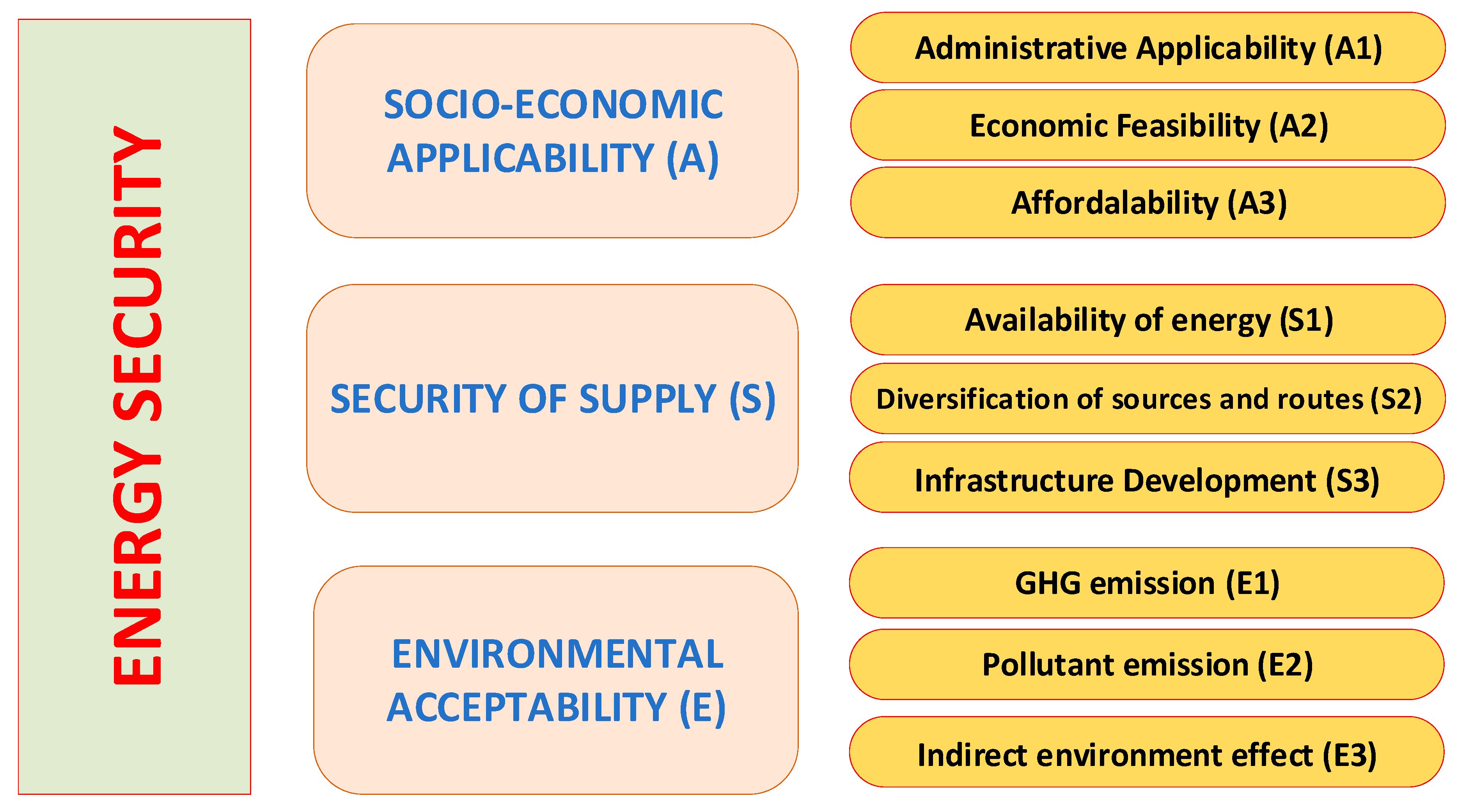
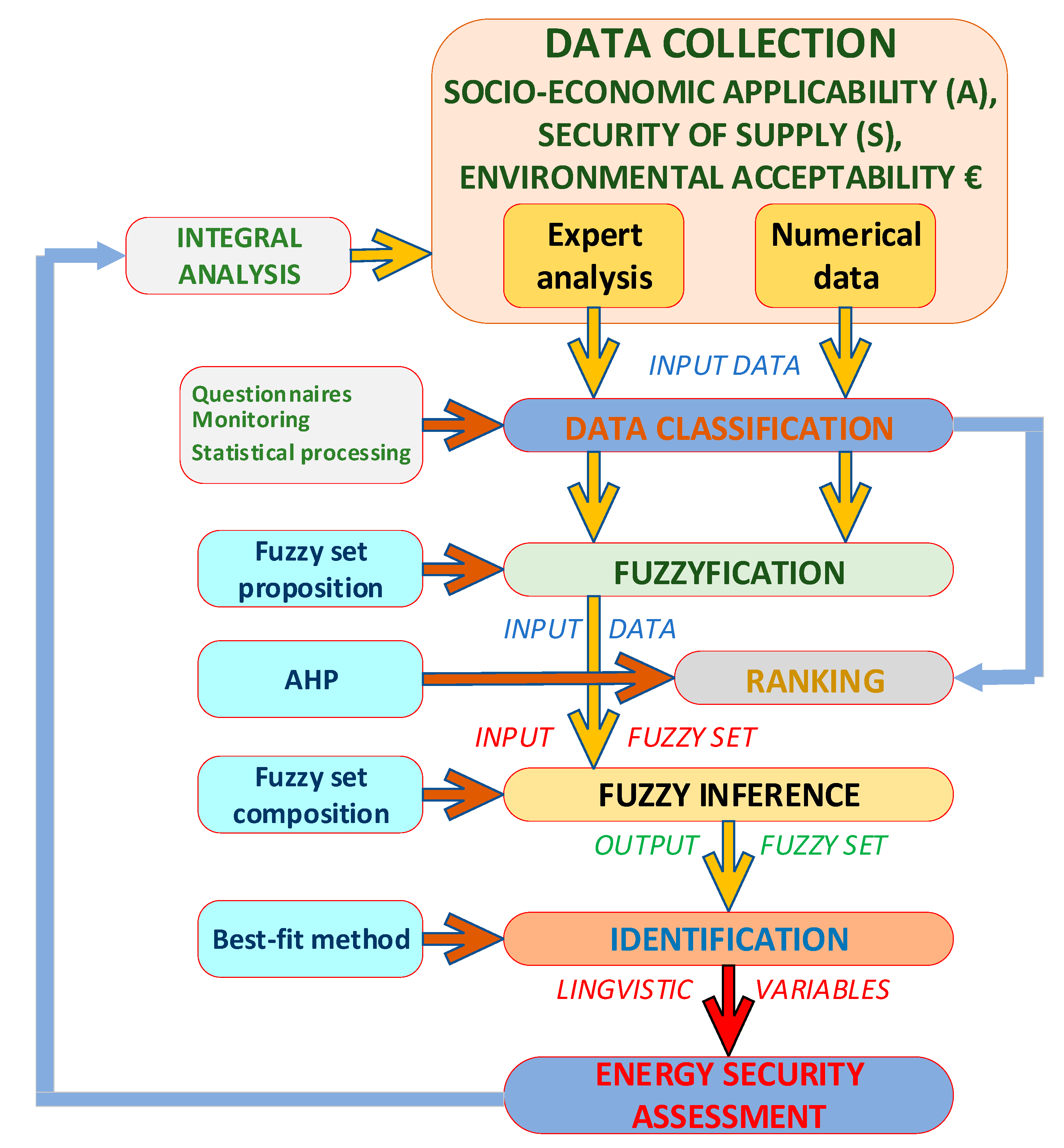
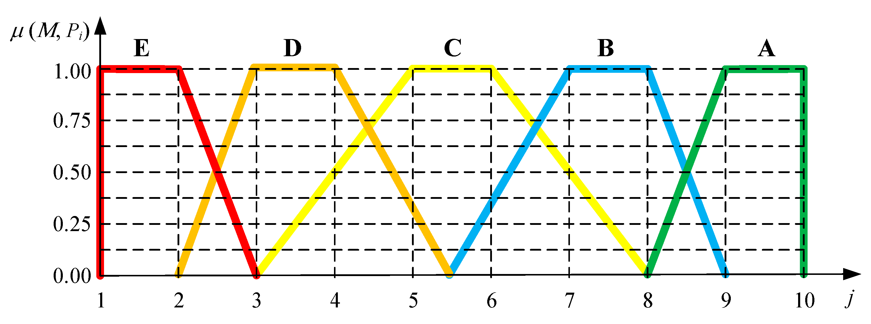
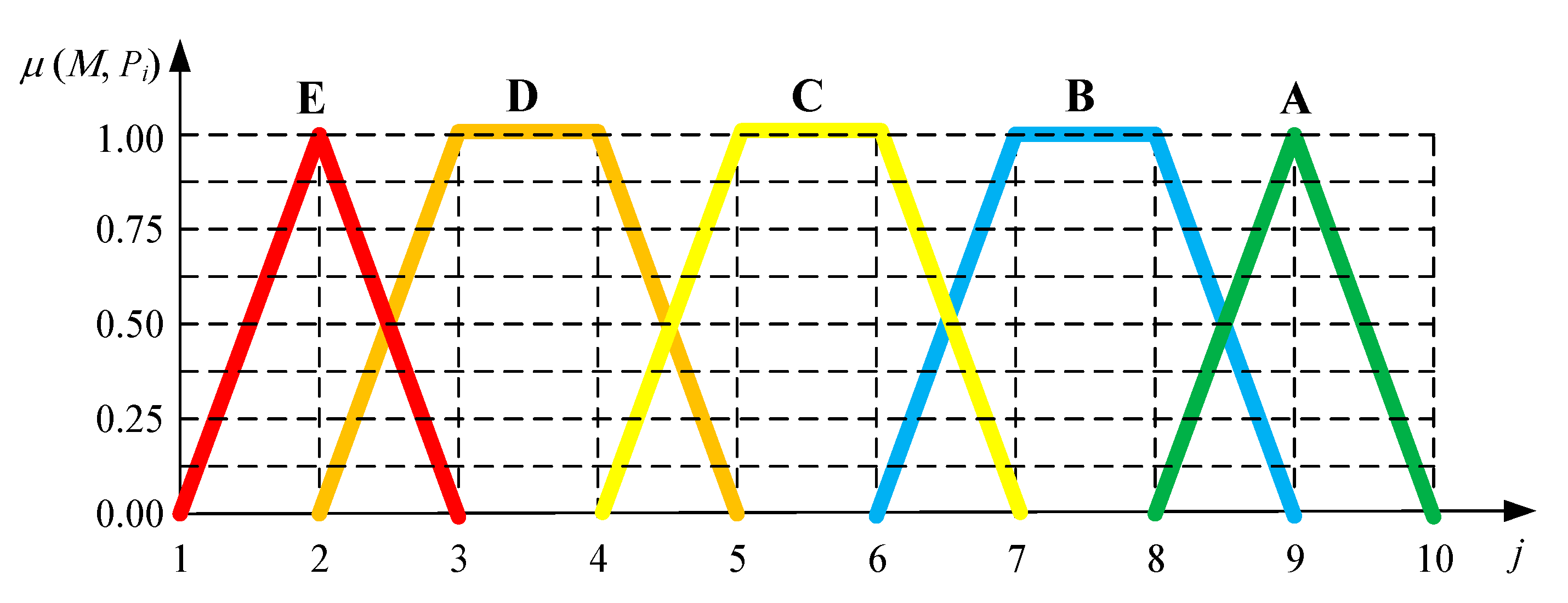
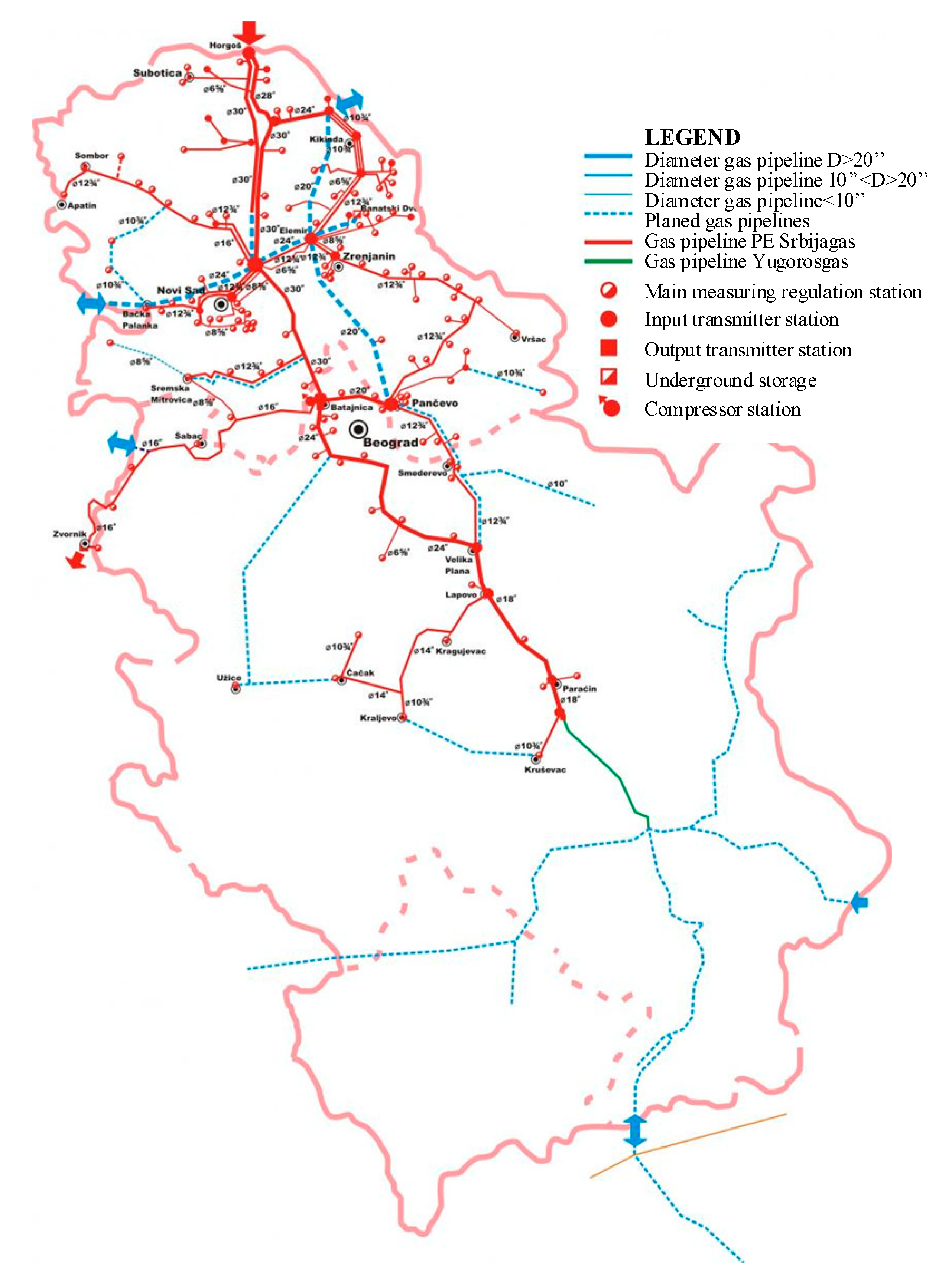
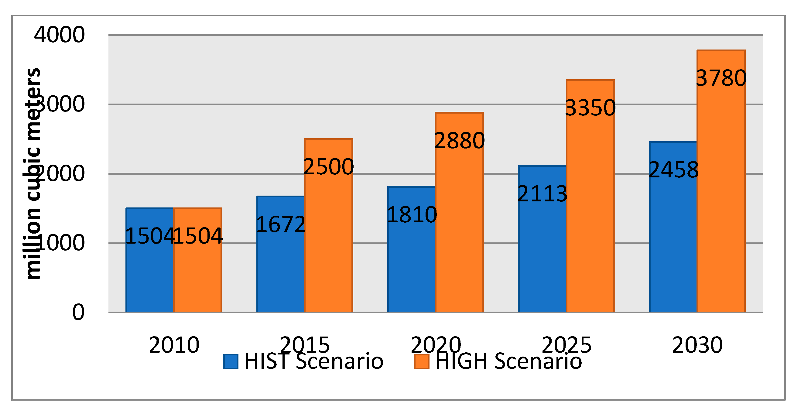
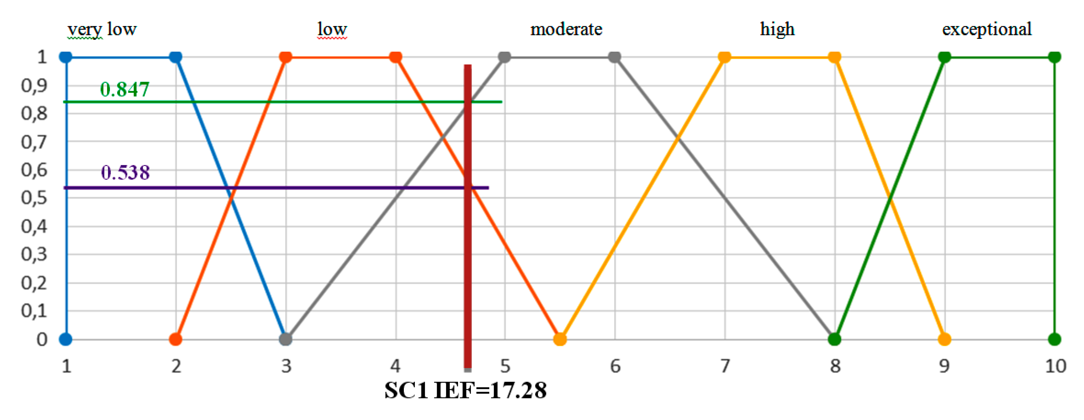
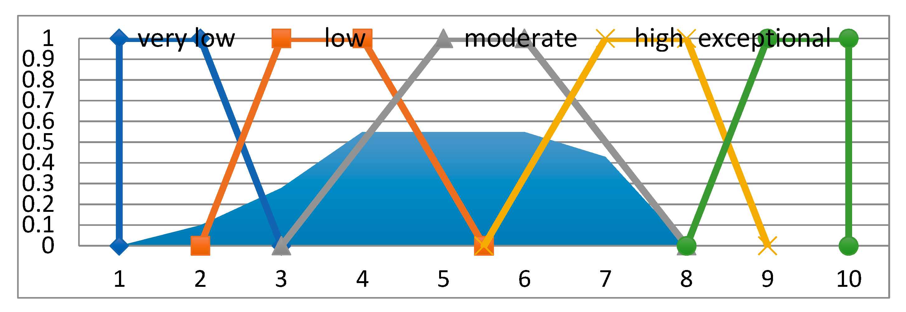
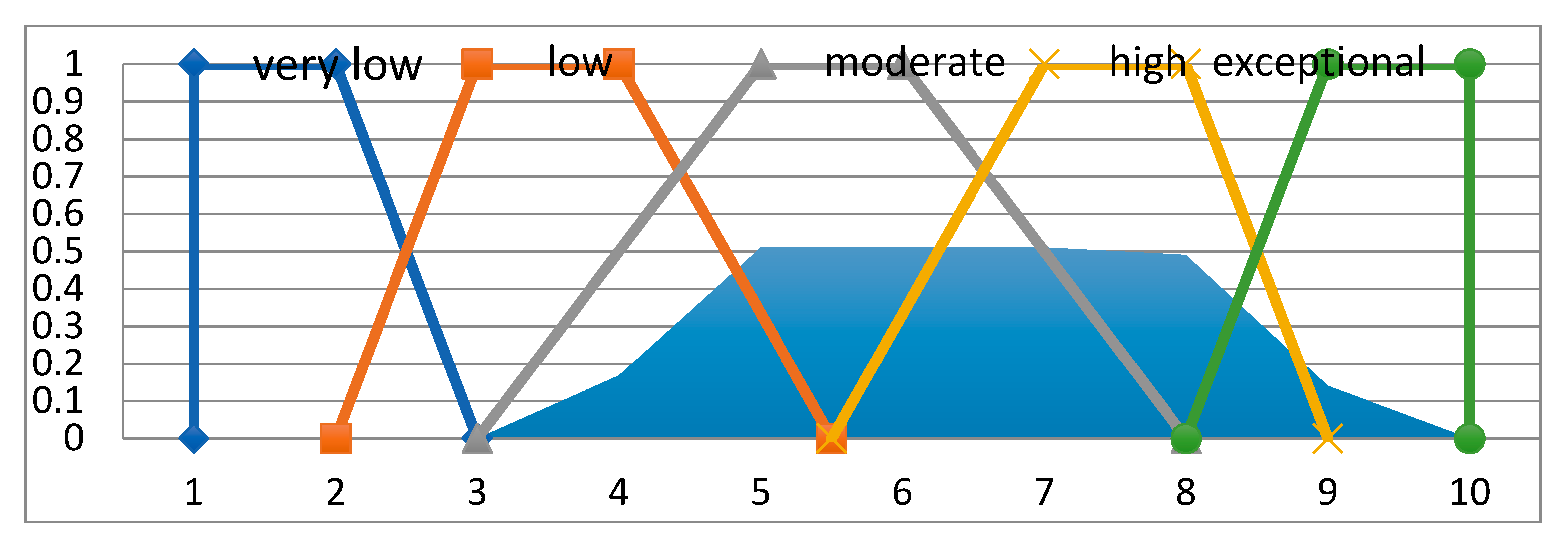
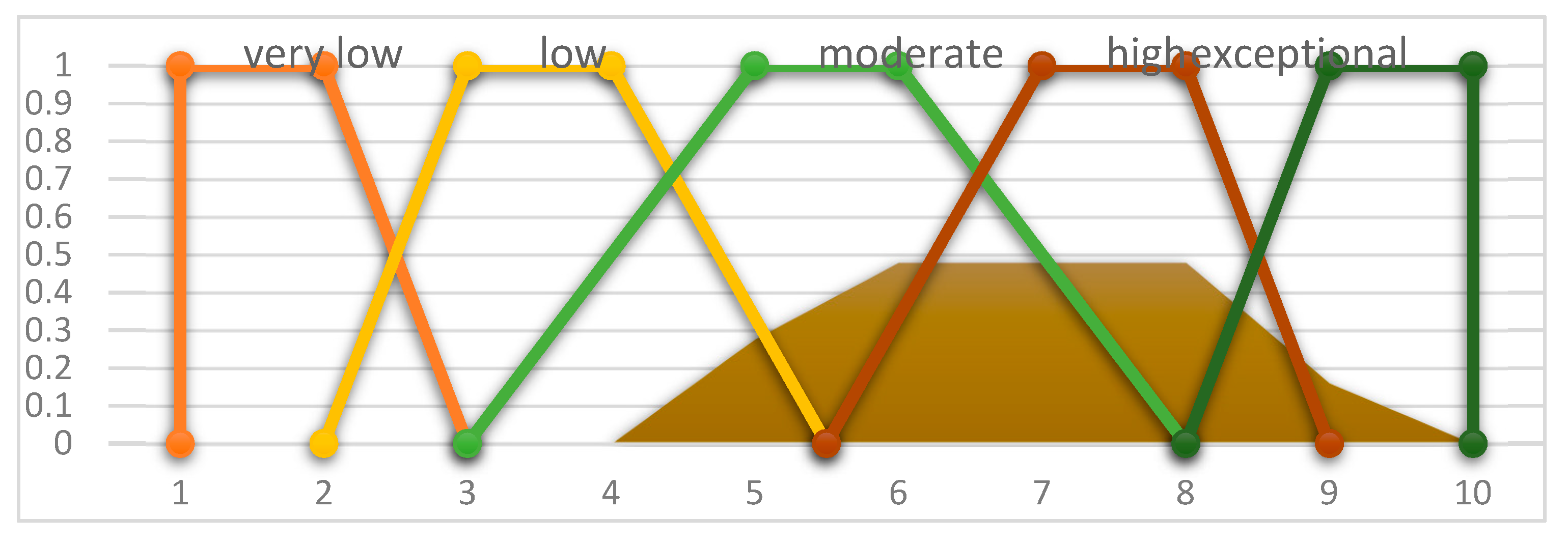
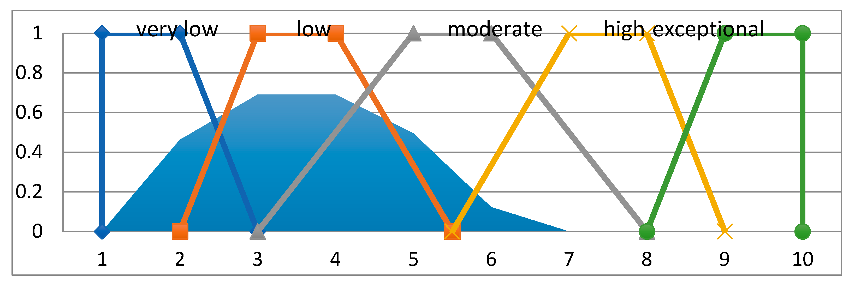
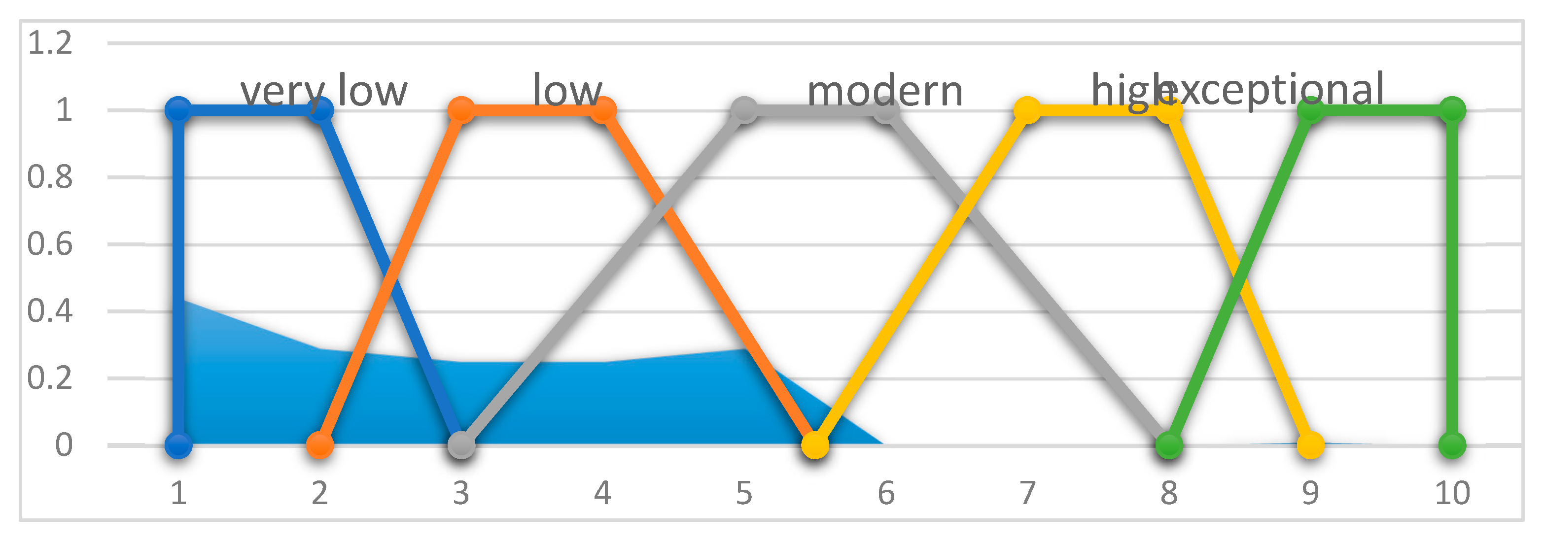
Table 1.
Partial indicators.
| Synthesis Indicators | Partial Indicator | Description | Fuzzification of Input Data |
|---|---|---|---|
| Socioeconomic applicability | Administrative applicability | It is the readiness and operability of human resources to create, support, improve and ensure the execution of certain operations that will enable the realization of the energy scenario. Lack of adequate staff can be an obstacle to the implementation of measures that provide for certain scenarios of energy development. administrative applicability is defined as a set of all actions carried out by employees in relevant institutions to implement measures concerning an energy scenario [2]. It involves the coordination of several different sectors, as well as various levels of governance and decision-making within multiple institutions, assigning obligations to specific public entities, timely and adequate inclusion of all relevant factors, etc. Capacity is based on professional staff, possessing the necessary technical aids and the transparency of the results of the work done [38]. | Expert analysis—questionnaires |
| Economic feasibility | Partial indicator economic feasibility looks at generating economic growth and increasing GDP. Economic development raises the level of energy security because the energy entity that is developing economically has greater opportunities to buy energy and therefore easier to create new values. economic feasibility is primarily considered in the analysis from the point of view of an energy company, investor or state. economic feasibility can also be seen as a measure of energy efficiency through increased consumption of natural gas. | Index EF—ratio of the degree of utilization of new capacities, i.e., use of energy and money invested IEF = degree of utilization/investment | |
| Affordability (end-user side) | The degree of liberalization of the natural gas market, by monitoring the amount of natural gas sold in the free market in relation to the total consumption of natural gas. The number of entities involved in the sale of the market is very important. | Herfindahl–Hirschman Index (HHI) indicating the level of free market concentration and it is calculated as the sum of the squares of the percentage (pi) of individual companies in the market. | |
| Security of Supply | Availability of energy | System availability index (N-1) indicating the daily operational flexibility, which describes the daily operational flexibility of the gas pipeline system, as well as the ability of the system to respond to consumption requirements in extreme conditions. | System availability index (N-1) includes technical pipeline capacity, domestic production, storage options and delivery from LPG terminals |
| Diversification of sources and routes | Diversification of sources and routes is an indicator which indicates the number of natural gas sources and the different directions through which natural gas can enter the country. The index of diversification of import rights of supply (IDIRS) [57] diversifies the import rights of supplies and depends on the available interconnection capacity. The lower the value of the index, the greater the diversification of sources and the direction of natural gas supply [58]. | IDIRS—Index of diversification of import rights of supply | |
| Development of gas infrastructure | It reflects the degree of gasification of the Republic of Serbia. This partial indicator shows the creation or stagnation of infrastructure prerequisites (transport systems) for the use of natural gas in parts of the country where it is not currently possible, as well as the construction of new and the development of an existing natural gas distribution network, which enables increased use and development of the domestic natural gas market. | DRIP—Degree of realization of planned infrastructure projects | |
| Environmental acceptability | GHG emission | Universal ecological indicator that monitors all anthropogenic impacts that result in greenhouse gas emissions. Effective monitoring and reporting of greenhouse gas emissions is the basis for progress in achieving emission reduction. | Coefficients of CO2 emission per unit of energy produced are used, due to different contribution to greenhouse gas emissions, primarily carbon dioxide [kgCO2/GJ]. |
| Emission of pollutants | Partial indicator which describes the type, intensity and mode of emission of the remaining pollutants (solid particles, NOx, SOx, COx, VOC, etc.) | Pollutant emission factors per unit of energy produced are used [g pol/GJ]. | |
| The indirect environment effect | Partial indicator of the accompanying effect of the use of natural gas on other energy products, i.e., the structure of energy use and energy efficiency measures. Natural gas appliances are more efficient, characterized by compact structure, lower costs of exploitation and low investment costs. Usage of natural gas also impacts on the environment also through the fact that there are no needs to build storage. | Expert analysis—questionnaires |
Table 2.
Production of natural gas [71].
Table 2.
Production of natural gas [71].
| Year | 2012 | 2013 | 2014 | 2015 | 2016 | 2017 | 2018 |
|---|---|---|---|---|---|---|---|
| Production (million m3) | 484 | 468 | 467 | 432 | 399 | 377 | 335 |
Table 3.
Transmitted natural gas quantities [71].
Table 3.
Transmitted natural gas quantities [71].
| Transmitted Natural Gas (million m3) | 2015 | 2016 | 2017 | 2018 |
|---|---|---|---|---|
| Production on the transmission system | 422 | 388 | 366 | 327 |
| Entry into Serbia from Hungary to meet Serbia’s demand | 1740 | 1795 | 2182 | 2146 |
| Entry into Serbia to meet Bosnia and Herzegovina’s demand | 223 | 232 | 265 | 304 |
| Total | 2386 | 2415 | 2813 | 2777 |
| From storage | 113 | 254 | 227 | 298 |
| Total | 2499 | 2669 | 3040 | 3075 |
Table 4.
Serbian natural gas infrastructure—main characteristics.
| Transmission System—Technical Information [71] | ||
|---|---|---|
| Transmission operator | PC Srbijagas | Yugorosgaz-Transport |
| Capacity, million m3/day | 18 * | ~2.2 |
| Pressure, bar | 16–75 | 16–55 |
| Length, km | 2339 | 125 |
| Diameter | DN 150–DN 750 | DN 168–DN 530 |
| Compressor station, МW | 4.4 | – |
| Metering and regulating stations | 248 | 5 |
| Number of entries into the transmission system | PC Srbijagas | Yugorosgaz-Transport |
| From another transmission system | 1 (Hungary) | 1 (PC Srbijagas) |
| Indigenous production | 11 | – |
| Storage | 1 | – |
| Interconnectors towards Bosnia and Herzegovina | 1 | – |
| Distributive network—technical information [71] | ||
| Number of gas entrance to distributive network | 242 | 5 |
| Number of delivery points | 276,581 ** | |
| Households | 262,814 | |
| District heating companies | 133 | |
| Industry and other | 13,634 | |
| Network characteristics | ||
| Length, km | 18,422 | |
| Operating pressure for industry (medium pressure) | 4–16 bar | |
| Length of distribution network at medium pressure | ~1470 km | |
| Operating pressure for households (low pressure) | <4 bar | |
| Length of distribution network at low pressure | ~16,950 km | |
* maximal daily capacity guaranteed by Hungarian transporter; ** There were 52 delivery points on the transmission system.
Table 5.
Natural gas consumption demand projection until 2030 [73].
Table 5.
Natural gas consumption demand projection until 2030 [73].
| Scenario | HIST Scenario | HIGH Scenario | ||||
|---|---|---|---|---|---|---|
| Projections | 2020 | 2025 | 2030 | 2020 | 2025 | 2030 |
| Households | 270 | 305 | 352 | 342 | 379 | 448 |
| District Heat Companies | 602 | 642 | 702 | 683 | 767 | 924 |
| Industry and others | 938 | 1130 | 1404 | 1855 | 2203 | 2408 |
Table 6.
Combined scenario of future natural gas development.
| Combined Scenarios | Scenarios of Infrastructure Development | Scenarios of Natural Gas Consumption |
|---|---|---|
| SC1 | BAU | HIST scenario |
| SC2 | BAU | HGH scenario |
| SC3 | OPT | HIST scenario |
| SC4 | OPT | HGH scenario |
| SC5 | PES | HIST scenario |
| SC6 | PES | HGH scenario |
These six combined scenarios were analyzed in order to evaluate energy security assessment.
Table 7.
Expert analysis for combined scenario 1 (SC1).
| Partial Indicator (Pi) | Administrative Applicability (A1) | Indirect Environment Effect (E3) | ||||||||
|---|---|---|---|---|---|---|---|---|---|---|
| LV | very low | Low | Moderate | High | exceptional | very negative | Negative | neutral | positive | very positive |
| Analyst 1 | 0.2 | 0.3 | 0.5 | 0.25 | 0.5 | 0.25 | ||||
| Analyst 2 | 0.1 | 0.5 | 0.4 | 0.5 | 0.3 | 0.2 | ||||
| Analyst 3 | 0.8 | 0.2 | 0.4 | 0.4 | 0.2 | |||||
| Analyst 4 | 0.1 | 0.5 | 0.3 | 0.1 | 0.6 | 0.4 | ||||
| Analyst 5 | 0.7 | 0.2 | 0.1 | 0.2 | 0.5 | 0.3 | ||||
| Results of expert analysis | E | D | C | B | A | E | D | C | B | A |
| (0.2 + 0.1 + 0.1)/5 | (0.3 + 2 × 0.5 + 0.8 + 0.7)/5 | (0.5 + 0.4 + 2 × 0.2 + 0.3)/5 | (0.1 + 0.1)/5 | 0 | 0 | (0.25 + 0.5 + 0.4 + 0.2)/5 | (2 × 0.5 + 0.4 + 0.3 + 0.6)/5 | (0.25 + 2 × 0.2 + 0.4 + 0.3)/5 | 0 | |
| n = 5 | 0.08 | 0.56 | 0.32 | 0.04 | 0 | 0 | 0.27 | 0.46 | 0.27 | 0 |
Table 8.
Specific fuzzy values for the partial indicator administrative applicability (A1) for combined scenario 1 (SC1).
Table 8.
Specific fuzzy values for the partial indicator administrative applicability (A1) for combined scenario 1 (SC1).
| J | 0 | 2 | 3 | 4 | 5 | 6 | 7 | 8 | 9 | 10 | |
|---|---|---|---|---|---|---|---|---|---|---|---|
| LV | |||||||||||
| very low | 0.08 | 0.08 | 0 | 0 | 0 | 0 | 0 | 0 | 0 | 0 | |
| Low | 0 | 0 | 0.56 | 0.56 | 0.1848 | 0 | 0 | 0 | 0 | 0 | |
| Moderate | 0 | 0 | 0 | 0.16 | 0.32 | 0.32 | 0.16 | 0 | 0 | 0 | |
| High | 0 | 0 | 0 | 0 | 0 | 0.0132 | 0.04 | 0.04 | 0 | 0 | |
| Exceptional | 0 | 0 | 0 | 0 | 0 | 0 | 0 | 0 | 0 | 0 | |
| μA1-SC1 | 0.08 | 0.08 | 0.56 | 0.72 | 0.5048 | 0.3332 | 0.2 | 0.04 | 0 | 0 | |
Table 9.
Specific fuzzy values for partial indicator indirect environmental effect (E3) for combined scenario 1 (SC1).
Table 9.
Specific fuzzy values for partial indicator indirect environmental effect (E3) for combined scenario 1 (SC1).
| j | 1 | 2 | 3 | 4 | 5 | 6 | 7 | 8 | 9 | 10 | |
|---|---|---|---|---|---|---|---|---|---|---|---|
| LV | |||||||||||
| very negative | 0 | 0 | 0 | 0 | 0 | 0 | 0 | 0 | 0 | 0 | |
| Negative | 0 | 0 | 0.27 | 0.27 | 0.089 | 0 | 0 | 0 | 0 | 0 | |
| Neutral | 0 | 0 | 0 | 0.23 | 0.46 | 0.46 | 0.23 | 0 | 0 | 0 | |
| Positive | 0 | 0 | 0 | 0 | 0 | 0.089 | 0.27 | 0.27 | 0 | 0 | |
| very positive | 0 | 0 | 0 | 0 | 0 | 0 | 0 | 0 | 0 | 0 | |
| μE3-SC1 | 0 | 0 | 0.27 | 0.5 | 0.549 | 0.549 | 0.5 | 0.27 | 0 | 0 | |
Table 10.
Expert analysis of partial indicators A1 and E3 using combined scenario questionnaires.
| Partial Indicator (Pi) | Administrative Applicability (A1) | Indirect Environment Effect (E3) | |||||||||
|---|---|---|---|---|---|---|---|---|---|---|---|
| LV | very low | low | Moderate | high | Exceptional | very negative | Negative | neutral | positive | very positive | |
| Combined scenario SC 2 | Analyst 1 | 0.4 | 0.5 | 0.1 | 0.5 | 0.5 | |||||
| Analyst 2 | 0.5 | 0.4 | 0.1 | 0.1 | 0.6 | 0.3 | |||||
| Analyst 3 | 0.7 | 0.2 | 0.1 | 0.3 | 0.7 | ||||||
| Analyst 4 | 0.4 | 0.4 | 0.2 | 0.8 | 0.2 | ||||||
| Analyst 5 | 0.1 | 0.4 | 0.5 | 1 | |||||||
| J | 0.02 | 0.48 | 0.4 | 0.1 | 0 | 0 | 0.08 | 0.72 | 0.2 | 0 | |
| μA1-SC2 | 0.02 | 0.02 | 0.48 | 0.68 | 0.56 | 0.43 | 0.3 | 0.1 | 0 | 0 | |
| μE3-SC2 | 0 | 0 | 0.08 | 0.44 | 0.75 | 0.79 | 0.56 | 0.2 | 0 | 0 | |
| Combined scenario SC 3 | Analyst 1 | 0.6 | 0.4 | 0.5 | 0.4 | 0.1 | |||||
| Analyst 2 | 0.5 | 0.5 | 0.1 | 0.6 | 0.3 | ||||||
| Analyst 3 | 0.3 | 0.7 | 0.6 | 0.4 | |||||||
| Analyst 4 | 0.9 | 0.1 | 0.1 | 0.5 | 0.4 | ||||||
| Analyst 5 | 0.3 | 0.5 | 0.2 | 0.6 | 0.4 | ||||||
| J | 0.22 | 0.64 | 0.14 | 0 | 0 | 0.02 | 0.34 | 0.48 | 0.16 | 0 | |
| μA1-SC3 | 0.22 | 0.22 | 0.64 | 0.71 | 0.35 | 0.14 | 0.07 | 0 | 0 | 0 | |
| μE3-SC3 | 0 | 0 | 0.08 | 0.44 | 0.75 | 0.79 | 0.56 | 0.2 | 0 | 0 | |
| Combined scenario SC 4 | Analyst 1 | 0.5 | 0.2 | 0.3 | 0.4 | 0.6 | |||||
| Analyst 2 | 0.3 | 0.5 | 0.2 | 0.2 | 0.4 | 0.3 | |||||
| Analyst 3 | 0.3 | 0.6 | 0.1 | 1 | |||||||
| Analyst 4 | 0.2 | 0.8 | 0.2 | 0.8 | |||||||
| Analyst 5 | 0.9 | 0.1 | 0.1 | 0.2 | 0.7 | ||||||
| J | 0.26 | 0.6 | 0.14 | 0 | 0 | 0 | 0 | 0.06 | 0.44 | 0.48 | |
| μA1-SC4 | 0.02 | 0.02 | 0.34 | 0.58 | 0.59 | 0.53 | 0.4 | 0.16 | 0 | 0 | |
| μE3-SC4 | 0 | 0 | 0 | 0.03 | 0.06 | 0.21 | 0.47 | 0.44 | 0.48 | 0.48 | |
| Combined scenario SC 5 | Analyst 1 | 0.5 | 0.4 | 0.1 | 0.6 | 0.4 | |||||
| Analyst 2 | 0.6 | 0.4 | 0.8 | 0.2 | |||||||
| Analyst 3 | 0.1 | 0.9 | 0.7 | 0.3 | |||||||
| Analyst 4 | 0.2 | 0.8 | 0.6 | 0.3 | 0.1 | ||||||
| Analyst 5 | 0.8 | 0.2 | 0.8 | 0.2 | |||||||
| J | 0.28 | 0.66 | 0.06 | 0 | 0 | 0.7 | 0.28 | 0.02 | 0 | 0 | |
| μA1-SC5 | 0.28 | 0.28 | 0.66 | 0.69 | 0.28 | 0.06 | 0.03 | 0 | 0 | 0 | |
| μE3-SC5 | 0.7 | 0.7 | 0.28 | 0.29 | 0.11 | 0.02 | 0.01 | 0 | 0 | 0 | |
| Combined scenario SC 6 | Analyst 1 | 1 | 0.6 | 0.4 | |||||||
| Analyst 2 | 0.5 | 0.5 | 0.8 | 0.2 | |||||||
| Analyst 3 | 0.5 | 0.4 | 0.1 | 1 | |||||||
| Analyst 4 | 0.6 | 0.4 | 0.6 | 0.4 | |||||||
| Analyst 5 | 0.4 | 0.6 | 0.7 | 0.3 | |||||||
| J | 0.4 | 0.58 | 0.02 | 0 | 0 | 0.74 | 0.26 | 0 | 0 | 0 | |
| μA1-SC6 | 0.4 | 0.4 | 0.58 | 0.59 | 0.21 | 0.02 | 0.01 | 0 | 0 | 0 | |
| μE3-SC6 | 0.74 | 0.74 | 0.26 | 0.26 | 0.09 | 0 | 0 | 0 | 0 | 0 | |
Table 11.
The values of the IEF for different scenarios for A2 partial indicator.
| A2 | SC 1 | SC 2 | SC 3 | SC 4 | SC 5 | SC 6 |
|---|---|---|---|---|---|---|
| Index EF (m3/€) | 17.28 | 13.82 | 20.58 | 25.73 | 32 | 40 |
Table 12.
Values for class j for partial indicators.
| J | A2 | A3 | S1 | S2 | S3 | E1 | E2 |
|---|---|---|---|---|---|---|---|
| IEF | HHI | N-1 | IDUPS | SRIP | 103 t CO2 | gpol/GJ | |
| 1 | 1 | 10,000 | 0.010 | 10,000 | 0 | 7000 | 467.83 |
| 2 | 5.333 | 8889 | 0.192 | 8889 | 0.111 | 6444 | 415.85 |
| 3 | 9.667 | 7778 | 0.374 | 7778 | 0.222 | 5889 | 363.87 |
| 4 | 14.000 | 6667 | 0.557 | 6667 | 0.333 | 5333 | 311.89 |
| 5 | 18.333 | 5556 | 0.739 | 5556 | 0.444 | 4778 | 259.91 |
| 6 | 22.667 | 4445 | 0.921 | 4445 | 0.556 | 4222 | 207.93 |
| 7 | 27.000 | 3334 | 1.103 | 3334 | 0.667 | 3667 | 155.94 |
| 8 | 31.333 | 2223 | 1.286 | 2223 | 0.778 | 3111 | 103.96 |
| 9 | 35.667 | 1112 | 1.468 | 1112 | 0.889 | 2556 | 51.98 |
| 10 | 40 | 1 | 1.650 | 1 | 1 | 2000 | 0 |
Table 13.
Specific fuzzy set values for the partial indicator economic feasibility (A2) for combined scenario SC1.
Table 13.
Specific fuzzy set values for the partial indicator economic feasibility (A2) for combined scenario SC1.
| j | 1 | 2 | 3 | 4 | 5 | 6 | 7 | 8 | 9 | 10 | |
|---|---|---|---|---|---|---|---|---|---|---|---|
| LV | |||||||||||
| E | 1·0 | 1·0 | 0·0 | 0·0 | 0·0 | 0·0 | 0·0 | 0·0 | 0·0 | 0·0 | |
| D | 0·0.388 | 0·0.388 | 1·0.388 | 1·0.388 | 0.33·0.388 | 0·0.388 | 0·0.388 | 0·0.388 | 0·0.388 | 0·0.388 | |
| C | 0·0.612 | 0·0.612 | 0·0.612 | 0.5·0.612 | 1·0.612 | 1·0.612 | 0.5·0.612 | 0·0.612 | 0·0.612 | 0·0.612 | |
| B | 0·0 | 0·0 | 0·0 | 0·0 | 0·0 | 0.33·0 | 1·0 | 1·0 | 0·0 | 0·0 | |
| A | 0·0 | 0·0 | 0·0 | 0·0 | 0·0 | 0·0 | 0·0 | 0·0 | 1·0 | 1·0 | |
| μA2-SC1 | 0 | 0 | 0.388 | 0.694 | 0.740 | 0.612 | 0.306 | 0 | 0 | 0 | |
Table 14.
Specific fuzzy set values for the partial indicator economic feasibility (A2) for combined scenarios SC2–SC6.
Table 14.
Specific fuzzy set values for the partial indicator economic feasibility (A2) for combined scenarios SC2–SC6.
| SC | 1 | 2 | 3 | 4 | 5 | 6 | 7 | 8 | 9 | 10 |
|---|---|---|---|---|---|---|---|---|---|---|
| μA2-SC2 | 0 | 0 | 0.904 | 0.952 | 0.394 | 0.096 | 0.048 | 0 | 0 | 0 |
| μA2-SC3 | 0 | 0 | 0 | 0.472 | 0.943 | 0.962 | 0.528 | 0.057 | 0 | 0 |
| μA2-SC4 | 0 | 0 | 0 | 0.243 | 0.486 | 0.655 | 0.757 | 0.514 | 0 | 0 |
| μA2-SC5 | 1 | 1 | 0 | 0 | 0 | 0 | 0 | 0 | 0 | 0 |
| μA2-SC6 | 1 | 1 | 0 | 0 | 0 | 0 | 0 | 0 | 0 | 0 |
Table 15.
Herfindahl–Hirschman index (HHI) value for combined development scenarios.
| A3 | SC 1 | SC 2 | SC 3 | SC 4 | SC 5 | SC 6 |
|---|---|---|---|---|---|---|
| HHIWHOLESALE | 5427 | 4918 | 4243 | 3512 | 6985 | 6312 |
| HHIRETAIL | 5287 | 4826 | 4112 | 3375 | 6915 | 6324 |
Table 16.
The specific fuzzy set values for the partial indicator affordability (A3) for combined scenarios SC1–SC6.
Table 16.
The specific fuzzy set values for the partial indicator affordability (A3) for combined scenarios SC1–SC6.
| j | 1 | 2 | 3 | 4 | 5 | 6 | 7 | 8 | 9 | 10 | |
|---|---|---|---|---|---|---|---|---|---|---|---|
| SC | |||||||||||
| μA3-SC1 | 0 | 0 | 0.143 | 0.572 | 0.904 | 0.857 | 0.428 | 0 | 0 | 0 | |
| μA2-SC2 | 0 | 0 | 0 | 0.462 | 0.924 | 0.949 | 0.538 | 0.076 | 0 | 0 | |
| μA2-SC3 | 0 | 0 | 0 | 0.289 | 0.577 | 0.717 | 0.711 | 0.423 | 0 | 0 | |
| μA2-SC4 | 0 | 0 | 0 | 0.204 | 0.408 | 0.603 | 0.796 | 0.592 | 0 | 0 | |
| μA2-SC5 | 0 | 0 | 0.755 | 0.877 | 0.494 | 0.245 | 0.123 | 0 | 0 | 0 | |
| μA2-SC6 | 0 | 0 | 0.556 | 0.778 | 0.627 | 0.444 | 0.222 | 0 | 0 | 0 | |
Table 17.
N-1 system availability index for different combination of scenarios.
| Scenarios for Natural Gas Infrastructure Development | BAU | PES | OPT | |||
|---|---|---|---|---|---|---|
| Projection of Natural gas Use [million m3 per day] | HIST Scenario | HIGH Scenario | HIST Scenario | HIGH Scenario | HIST Scenario | HIGH Scenario |
| TPC | 15.93 | 11 | 24.41 | |||
| IPG 2016 | 1.11 | |||||
| IPG 2020 | 1.105 | |||||
| IPG 2025 | 0.78 | |||||
| MWUS | 9.96 | 4.95 | 9.96 | |||
| MW LNG | 0 | |||||
| LGI | 11 | |||||
| MDC 2016 | 14.9 | |||||
| MDC 2020 | 16.08 | 18.98 | 16.08 | 18.98 | 16.08 | 18.98 |
| MDC 2025 | 17.23 | 21.79 | 17.23 | 21.79 | 17.23 | 21.79 |
| N-1 2016 | 1.10 * | 1.10 * | 0.42 | 0.42 | 1.69* | 1.69 * |
| N-1 2020 | 0.99 | 0.84 | 0.38 | 0.32 | 1.52 | 1.29 |
| N-1 2025 | 0.91 | 0.72 | 0.33 | 0.26 | 1.40 | 1.11 |
* hypothetical value—selected infrastructure does not exist.
Table 18.
Specific fuzzy set values for the partial indicator availability of energy (S1) for combined scenarios SC1–SC6.
Table 18.
Specific fuzzy set values for the partial indicator availability of energy (S1) for combined scenarios SC1–SC6.
| j | 1 | 2 | 3 | 4 | 5 | 6 | 7 | 8 | 9 | 10 | |
|---|---|---|---|---|---|---|---|---|---|---|---|
| SC | |||||||||||
| μS1-SC1 | 0 | 0 | 0 | 0.500 | 1.000 | 1.000 | 0.500 | 0 | 0 | 0 | |
| μS1-SC2 | 0 | 0 | 0 | 0.500 | 1.000 | 1.000 | 0.500 | 0 | 0 | 0 | |
| μS1-SC3 | 0 | 0 | 0 | 0 | 0 | 0 | 0 | 0 | 1 | 1 | |
| μS1-SC4 | 0 | 0 | 0 | 0 | 0 | 0.324 | 0.981 | 0.981 | 0.019 | 0.019 | |
| μS1-SC5 | 0 | 0 | 1 | 1 | 0.333 | 0 | 0 | 0 | 0 | 0 | |
| μS1-SC6 | 0.382 | 0.382 | 0.618 | 0.618 | 0.204 | 0 | 0 | 0 | 0 | 0 | |
Table 19.
Index of diversification of import rights of supply (IDIRS) in case of realization of the planned projects of interconnections.
Table 19.
Index of diversification of import rights of supply (IDIRS) in case of realization of the planned projects of interconnections.
| S2 | Current State | New Interconnections | Interconnections + LNG Terminal + New UGSs | ||
|---|---|---|---|---|---|
| Hungary | Bulgaria | Romania | Croatia | Complete Realization | |
| IDIRS | 10,000 | 6007 | 6224 | 6348 | 3282 |
Table 20.
Specific fuzzy set values for the partial indicator diversification of sources and routes (S2) for combined scenarios SC1–SC6.
Table 20.
Specific fuzzy set values for the partial indicator diversification of sources and routes (S2) for combined scenarios SC1–SC6.
| j | 1 | 2 | 3 | 4 | 5 | 6 | 7 | 8 | 9 | 10 | |
|---|---|---|---|---|---|---|---|---|---|---|---|
| SC | |||||||||||
| μS2-SC1 | 0 | 0 | 0.452 | 0.726 | 0.697 | 0.548 | 0.274 | 0 | 0 | 0 | |
| μS2-SC2 | 0 | 0 | 0.452 | 0.726 | 0.697 | 0.548 | 0.274 | 0 | 0 | 0 | |
| μS2-SC3 | 0 | 0 | 0 | 0.149 | 0.298 | 0.530 | 0.851 | 0.702 | 0 | 0 | |
| μS2-SC4 | 0 | 0 | 0 | 0.149 | 0.298 | 0.530 | 0.851 | 0.702 | 0 | 0 | |
| μS2-SC5 | 1 | 1 | 0 | 0 | 0 | 0 | 0 | 0 | 0 | 0 | |
| μS2-SC6 | 1 | 1 | 0 | 0 | 0 | 0 | 0 | 0 | 0 | 0 | |
Table 21.
Degree of realization of planned infrastructure projects (DRIP) index for the partial indicator infrastructure development (S3) for combined scenarios SC1–SC6.
Table 21.
Degree of realization of planned infrastructure projects (DRIP) index for the partial indicator infrastructure development (S3) for combined scenarios SC1–SC6.
| S3 | SC 1 | SC 2 | SC 3 | SC 4 | SC 5 | SC 6 |
|---|---|---|---|---|---|---|
| DRIP | 0.443 | 0.539 | 0.835 | 1 | 0.238 | 0 |
Table 22.
Specific fuzzy set values for the partial indicator infrastructure development (S3) for combined scenarios SC1–SC6.
Table 22.
Specific fuzzy set values for the partial indicator infrastructure development (S3) for combined scenarios SC1–SC6.
| j | 1 | 2 | 3 | 4 | 5 | 6 | 7 | 8 | 9 | 10 | |
|---|---|---|---|---|---|---|---|---|---|---|---|
| SC | |||||||||||
| μS3-SC1 | 0 | 0 | 0.279 | 0.639 | 0.813 | 0.721 | 0.361 | 0 | 0 | 0 | |
| μS3-SC2 | 0 | 0 | 0 | 0.459 | 0.917 | 0.944 | 0.541 | 0.083 | 0 | 0 | |
| μS3-SC3 | 0 | 0 | 0 | 0 | 0 | 0.168 | 0.510 | 0.510 | 0.490 | 0.490 | |
| μS3-SC4 | 0 | 0 | 0 | 0 | 0 | 0 | 0 | 0 | 1 | 1 | |
| μS3-SC5 | 0 | 0 | 0.865 | 0.933 | 0.420 | 0.135 | 0.067 | 0 | 0 | 0 | |
| μS3-SC6 | 1 | 1 | 0 | 0 | 0 | 0 | 0 | 0 | 0 | 0 | |
Table 23.
Projections of natural gas consumption and emission of CO2 and NOx.
| Scenario | HIST | HIGH | kCO2 kg/GJ | ||
|---|---|---|---|---|---|
| 56.1 | |||||
| kNOx g/GJ | |||||
| Sector | 2020 | 2025 | 2020 | 2025 | 0.1 |
| Households | 269.570 | 305.172 | 341.591 | 379.267 | million m3 |
| Heat Plant | 602.335 | 641.740 | 683.183 | 767.325 | |
| Industry | 938.095 | 1129.669 | 1855,226 | 2203.408 | |
| Total | 1810 | 2076.581 | 2880 | 3350 | |
| Heat power | 33.338 | 33.338 | 33.338 | 33.338 | MJ/m3 |
| Households | 8986925 | 10173824 | 11387961 | 12644003 | GJ |
| Heat Plant | 20080644 | 21394328 | 22775955 | 25581081 | |
| Industry | 31274211 | 37660905 | 61849524 | 73457215 | |
| Total | 60341780 | 69229057 | 96013440 | 111682300 | |
| Emissions CO2 | 3385174 | 3883750 | 5386354 | 6265377 | t CO2 |
| Emissions NOx | 6034 | 6923 | 9601 | 11,168 | kg NOx |
Table 24.
Numerical input data for partial indicator GHG emissions (E1).
| E1 | SC 1 | SC 2 | SC 3 | SC 4 | SC 5 | SC 6 |
|---|---|---|---|---|---|---|
| 103 t CO2 | 3385 | 5386 | 2877 | 3232 | 4401 | 6433 |
Table 25.
Specific fuzzy set values for the partial indicator GHG emissions (E1) for combined scenarios SC1–SC6.
Table 25.
Specific fuzzy set values for the partial indicator GHG emissions (E1) for combined scenarios SC1–SC6.
| j | 1 | 2 | 3 | 4 | 5 | 6 | 7 | 8 | 9 | 10 | |
|---|---|---|---|---|---|---|---|---|---|---|---|
| SC | |||||||||||
| μE1-SC1 | 0 | 0 | 0 | 0.098 | 0.196 | 0.461 | 0.902 | 0.804 | 0 | 0 | |
| μE1-SC2 | 0 | 0 | 0.675 | 0.837 | 0.548 | 0.325 | 0.163 | 0 | 0 | 0 | |
| μE1-SC3 | 0 | 0 | 0 | 0 | 0 | 0.170 | 0.514 | 0.514 | 0.486 | 0.486 | |
| μE1-SC4 | 0 | 0 | 0 | 0 | 0 | 0.277 | 0.839 | 0.839 | 0.161 | 0.161 | |
| μE1-SC5 | 0 | 0 | 0 | 0.463 | 0.925 | 0.950 | 0.537 | 0.075 | 0 | 0 | |
| μE1-SC6 | 0.926 | 0.926 | 0.074 | 0.074 | 0.024 | 0 | 0 | 0 | 0 | 0 | |
Table 26.
Numerical input data for partial indicator pollutant emissions (E2).
| E2 | SC 1 | SC 2 | SC 3 | SC 4 | SC 5 | SC 6 |
|---|---|---|---|---|---|---|
| kg NOx | 6034 | 9601 | 5123 | 5761 | 7844 | 11,526 |
Table 27.
Specific fuzzy set values for the partial indicator pollutant emissions (E2) for combined scenarios SC1–SC6.
Table 27.
Specific fuzzy set values for the partial indicator pollutant emissions (E2) for combined scenarios SC1–SC6.
| j | 1 | 2 | 3 | 4 | 5 | 6 | 7 | 8 | 9 | 10 | |
|---|---|---|---|---|---|---|---|---|---|---|---|
| SC | |||||||||||
| μE2-SC1 | 0 | 0 | 0 | 0 | 0 | 0.282 | 0.853 | 0.853 | 0.147 | 0.147 | |
| μE2-SC2 | 0 | 0 | 0.675 | 0.837 | 0.548 | 0.325 | 0.163 | 0.675 | 0 | 0 | |
| μE2-SC3 | 0 | 0 | 0 | 0 | 0 | 0.099 | 0.301 | 0.301 | 0.699 | 0.699 | |
| μE2-SC4 | 0 | 0 | 0 | 0.204 | 0.408 | 0.168 | 0.508 | 0.508 | 0.492 | 0.492 | |
| μE2-SC5 | 0 | 0 | 0.755 | 0.381 | 0.762 | 0.841 | 0.619 | 0.238 | 0 | 0 | |
| μE2-SC6 | 1 | 1 | 0 | 0 | 0 | 0 | 0 | 0 | 0 | 0 | |
Table 28.
Comparison of the influence of partials indicators on synthesis indicators, random consistency index and weight coefficients for different partial indicators.
Table 28.
Comparison of the influence of partials indicators on synthesis indicators, random consistency index and weight coefficients for different partial indicators.
| Socioeconomic applicability | A | administrative applicability | economic feasibility | affordability | CR | 0.071 | Wi% |
| administrative applicability | 1 | 2 | 0.142857 | 14.97 | |||
| economic feasibility | 0.5 | 1 | 0.166667 | 9.91 | |||
| affordability | 7 | 6 | 1 | 75.13 | |||
| Security of supply | S | availability of energy | Divers. sources and routes | infrastructure development | CR | 0.033 | Wi% |
| availability of energy | 1 | 0.333333 | 0.2 | 10.62 | |||
| Diversification sources and routes | 3 | 1 | 0.333333 | 26.05 | |||
| infrastructure development | 5 | 3 | 1 | 63.33 | |||
| environmental acceptability | E | GHG emission | pollutant emission | Indirect environmental effect | CR | 0.075 | Wi% |
| GHG emission | 1 | 3 | 5 | 61.94 | |||
| pollutant emission | 0.333333 | 1 | 4 | 28.42 | |||
| Indirect environmental effect | 0.2 | 0.25 | 1 | 9.64 |
Table 29.
Results of analysis for SC1.
| Social-Economic Applicability | 1 | 2 | 3 | 4 | 5 | 6 | 7 | 8 | 9 | 10 |
|---|---|---|---|---|---|---|---|---|---|---|
| Administrative Applicability | 0.080 | 0.080 | 0.560 | 0.720 | 0.505 | 0.333 | 0.200 | 0.040 | 0 | 0 |
| Economic Feasibility | 0 | 0 | 0.388 | 0.694 | 0.740 | 0.612 | 0.306 | 0 | 0 | 0 |
| Affordability | 0 | 0 | 0.143 | 0.572 | 0.904 | 0.857 | 0.428 | 0 | 0 | 0 |
| Security of Supply | 1 | 2 | 3 | 4 | 5 | 6 | 7 | 8 | 9 | 10 |
| Availability of energy | 0 | 0 | 0 | 0.5 | 1 | 1 | 0.5 | 0 | 0 | 0 |
| Diversifications of sources and routes | 0 | 0 | 0.452 | 0.726 | 0.697 | 0.548 | 0.274 | 0 | 0 | 0 |
| Infrastructure Development | 0 | 0 | 0.279 | 0.639 | 0.813 | 0.721 | 0.361 | 0 | 0 | 0 |
| Environmental Acceptability | 1 | 2 | 3 | 4 | 5 | 6 | 7 | 8 | 9 | 10 |
| GHG emissions | 0 | 0 | 0 | 0.098 | 0.196 | 0.461 | 0.902 | 0.804 | 0 | 0 |
| Pollutant emissions | 0 | 0 | 0 | 0 | 0 | 0.282 | 0.853 | 0.853 | 0.147 | 0.147 |
| Indirect environmental effect | 0 | 0 | 0.27 | 0,5 | 0.549 | 0.549 | 0.5 | 0.27 | 0 | 0 |
| Combined scenario 1 (SC1) | 1 | 2 | 3 | 4 | 5 | 6 | 7 | 8 | 9 | 10 |
| Socio-economic Applicability | 0 | 0.143 | 0.572 | 0.720 | 0.720 | 0.720 | 0.428 | 0 | 0 | 0 |
| Security of Supply | 0 | 0.279 | 0.639 | 0.726 | 0.726 | 0.697 | 0.361 | 0 | 0 | 0 |
| Environmental Acceptability | 0 | 0 | 0 | 0.098 | 0.196 | 0.461 | 0.549 | 0.549 | 0.147 | 0 |
| ENERGY SECURITY | 0 | 0.098 | 0.279 | 0.549 | 0.549 | 0.549 | 0.428 | 0 | 0 | 0 |
Table 30.
Results of the analysis for SC2.
| Social-Economic Applicability | 1 | 2 | 3 | 4 | 5 | 6 | 7 | 8 | 9 | 10 |
|---|---|---|---|---|---|---|---|---|---|---|
| Administrative Applicability | 0.020 | 0.020 | 0.480 | 0.680 | 0.558 | 0.433 | 0.300 | 0.100 | 0 | 0 |
| Economic Feasibility | 0 | 0 | 0.904 | 0.952 | 0.394 | 0.096 | 0.048 | 0 | 0 | 0 |
| Affordability | 0 | 0 | 0 | 0.462 | 0.924 | 0.949 | 0.538 | 0.076 | 0 | 0 |
| Security of Supply | 1 | 2 | 3 | 4 | 5 | 6 | 7 | 8 | 9 | 10 |
| Availability of energy | 0 | 0 | 0 | 0.5 | 1 | 1 | 0.5 | 0 | 0 | 0 |
| Diversifications of sources and routes | 0 | 0 | 0.452 | 0.726 | 0.697 | 0.548 | 0.274 | 0 | 0 | 0 |
| Infrastructure Development | 0 | 0 | 0 | 0.414 | 0.827 | 0.884 | 0.586 | 0.173 | 0 | 0 |
| Environmental Acceptability | 1 | 2 | 3 | 4 | 5 | 6 | 7 | 8 | 9 | 10 |
| GHG emissions | 0 | 0 | 0.675 | 0.837 | 0.548 | 0.325 | 0.163 | 0 | 0 | 0 |
| Pollutant emissions | 0 | 0 | 0.675 | 0.8378 | 0.5488 | 0.325 | 0.163 | 0 | 0 | 0 |
| Indirect environmental effect | 0 | 0 | 0.08 | 0.44 | 0.746 | 0.786 | 0.56 | 0.2 | 0 | 0 |
| Combined scenario 2 (SC2) | 1 | 2 | 3 | 4 | 5 | 6 | 7 | 8 | 9 | 10 |
| Socio-economic Applicability | 0 | 0 | 0.462 | 0.680 | 0.680 | 0.680 | 0.433 | 0.076 | 0 | 0 |
| Security of Supply | 0 | 0 | 0.414 | 0.726 | 0.726 | 0.697 | 0.548 | 0.173 | 0 | 0 |
| Environmental Acceptability | 0 | 0 | 0.675 | 0.786 | 0.548 | 0.325 | 0.163 | 0 | 0 | 0 |
| ENERGY SECURITY | 0 | 0 | 0.675 | 0.680 | 0.680 | 0.548 | 0.173 | 0 | 0 | 0 |
Table 31.
Results of analysis for SC3.
| Social-Economic Applicability | 1 | 2 | 3 | 4 | 5 | 6 | 7 | 8 | 9 | 10 |
|---|---|---|---|---|---|---|---|---|---|---|
| Administrative Applicability | 0.220 | 0.220 | 0.640 | 0.710 | 0.351 | 0.140 | 0.070 | 0 | 0 | 0 |
| Economic Feasibility | 0 | 0 | 0 | 0.472 | 0.943 | 0.962 | 0.528 | 0.057 | 0 | 0 |
| Affordability | 0 | 0 | 0 | 0.289 | 0.577 | 0.717 | 0.711 | 0.423 | 0 | 0 |
| Security of Supply | 1 | 2 | 3 | 4 | 5 | 6 | 7 | 8 | 9 | 10 |
| Availability of energy | 0 | 0 | 0 | 0 | 0 | 0 | 0 | 0 | 1 | 1 |
| Diversifications of sources and routes | 0 | 0 | 0 | 0.149 | 0.298 | 0.530 | 0.851 | 0.702 | 0 | 0 |
| Infrastructure Development | 0 | 0 | 0 | 0 | 0 | 0.168 | 0.510 | 0.510 | 0.490 | 0.490 |
| Environmental Acceptability | 1 | 2 | 3 | 4 | 5 | 6 | 7 | 8 | 9 | 10 |
| GHG emissions | 0 | 0 | 0 | 0 | 0 | 0.169 | 0.51 | 0.513 | 0.486 | 0.486 |
| Pollutant emissions | 0 | 0 | 0 | 0 | 0 | 0.099 | 0.301 | 0.301 | 0.698 | 0.698 |
| Indirect environmental effect | 0.02 | 0.02 | 0.4 | 0.58 | 0.592 | 0.533 | 0.4 | 0.16 | 0 | 0 |
| Combined scenario 3 (SC3) | 1 | 2 | 3 | 4 | 5 | 6 | 7 | 8 | 9 | 10 |
| Socio-economic Applicability | 0 | 0 | 0.289 | 0.577 | 0.710 | 0.710 | 0.528 | 0.140 | 0 | 0 |
| Security of Supply | 0 | 0 | 0 | 0 | 0.168 | 0.510 | 0.510 | 0.510 | 0.490 | 0 |
| Environmental Acceptability | 0 | 0 | 0 | 0 | 0 | 0.169 | 0.513 | 0.513 | 0.486 | 0.486 |
| ENERGY SECURITY | 0 | 0 | 0 | 0.168 | 0.51 | 0.51 | 0.51 | 0.49 | 0.14 | 0 |
Table 32.
Results of the analysis for SC4.
| Social-Economic Applicability | 1 | 2 | 3 | 4 | 5 | 6 | 7 | 8 | 9 | 10 |
|---|---|---|---|---|---|---|---|---|---|---|
| Administrative Applicability | 0.260 | 0.260 | 0.600 | 0.670 | 0.338 | 0.140 | 0.070 | 0 | 0 | 0 |
| Economic Feasibility | 0 | 0 | 0 | 0.243 | 0.486 | 0.655 | 0.757 | 0.514 | 0 | 0 |
| Affordability | 0 | 0 | 0 | 0.204 | 0.408 | 0.603 | 0.796 | 0.592 | 0 | 0 |
| Security of Supply | 1 | 2 | 3 | 4 | 5 | 6 | 7 | 8 | 9 | 10 |
| Availability of energy | 0 | 0 | 0 | 0 | 0 | 0.324 | 0.981 | 0.981 | 0.019 | 0.019 |
| Diversifications of sources and routes | 0 | 0 | 0 | 0.149 | 0.298 | 0.530 | 0.851 | 0.702 | 0 | 0 |
| Infrastructure Development | 0 | 0 | 0 | 0 | 0 | 0 | 0 | 0 | 1 | 1 |
| Environmental Acceptability | 1 | 2 | 3 | 4 | 5 | 6 | 7 | 8 | 9 | 10 |
| GHG emissions | 0 | 0 | 0 | 0 | 0 | 0.277 | 0.839 | 0.839 | 0.161 | 0.161 |
| Pollutant emissions | 0 | 0 | 0 | 0 | 0 | 0.168 | 0.508 | 0.508 | 0.492 | 0.492 |
| Indirect environmental effect | 0 | 0 | 0 | 0.030 | 0.060 | 0.205 | 0.470 | 0.440 | 0.480 | 0.480 |
| Combined scenario 4 (SC4) | 1 | 2 | 3 | 4 | 5 | 6 | 7 | 8 | 9 | 10 |
| Socio-economic Applicability | 0 | 0 | 0.204 | 0.408 | 0.603 | 0.670 | 0.670 | 0.338 | 0 | 0 |
| Security of Supply | 0 | 0 | 0 | 0 | 0 | 0 | 0.530 | 0.851 | 0.851 | 0 |
| Environmental Acceptability | 0 | 0 | 0 | 0 | 0 | 0.277 | 0.480 | 0.480 | 0.480 | 0.161 |
| ENERGY SECURITY | 0 | 0 | 0 | 0 | 0.277 | 0.48 | 0.48 | 0.48 | 0.385 | 0.161 |
Table 33.
Results of the analysis for SC5.
| Social-Economic Applicability | 1 | 2 | 3 | 4 | 5 | 6 | 7 | 8 | 9 | 10 |
|---|---|---|---|---|---|---|---|---|---|---|
| Administrative Applicability | 0.280 | 0.280 | 0.660 | 0.690 | 0.278 | 0.060 | 0.030 | 0.000 | 0.000 | 0.000 |
| Economic Feasibility | 1.000 | 1.000 | 0 | 0 | 0 | 0 | 0 | 0 | 0 | 0 |
| Affordability | 0 | 0 | 0.755 | 0.877 | 0.494 | 0.245 | 0.123 | 0 | 0 | 0 |
| Security of Supply | 1 | 2 | 3 | 4 | 5 | 6 | 7 | 8 | 9 | 10 |
| Availability of energy | 0 | 0 | 1 | 1 | 0.33 | 0 | 0 | 0 | 0 | 0 |
| Diversifications of sources and routes | 1 | 1 | 0 | 0 | 0 | 0 | 0 | 0 | 0 | 0 |
| Infrastructure Development | 0 | 0 | 0.865 | 0.933 | 0.420 | 0.135 | 0.067 | 0 | 0 | 0 |
| Environmental Acceptability | 1 | 2 | 3 | 4 | 5 | 6 | 7 | 8 | 9 | 10 |
| GHG emissions | 0 | 0 | 0 | 0.463 | 0.925 | 0.950 | 0.537 | 0.075 | 0 | 0 |
| Pollutant emissions | 0 | 0 | 0 | 0.381 | 0.762 | 0.841 | 0.619 | 0.238 | 0 | 0 |
| Indirect environmental effect | 0.700 | 0.700 | 0.280 | 0.290 | 0.112 | 0.020 | 0.010 | 0 | 0 | 0 |
| Combined scenario 5 (SC5) | 1 | 2 | 3 | 4 | 5 | 6 | 7 | 8 | 9 | 10 |
| Socio-economic Applicability | 0 | 0.690 | 0.690 | 0.690 | 0.494 | 0.123 | 0.030 | 0 | 0 | 0 |
| Security of Supply | 0 | 0.933 | 0.933 | 0.420 | 0.135 | 0 | 0 | 0 | 0 | 0 |
| Environmental Acceptability | 0 | 0 | 0 | 0.463 | 0.700 | 0.700 | 0.537 | 0.075 | 0 | 0 |
| ENERGY SECURITY | 0 | 0.463 | 0.69 | 0.69 | 0.494 | 0.123 | 0 | 0 | 0 | 0 |
Table 34.
Results of the analysis for SC6.
| Social-Economic Applicability | 1 | 2 | 3 | 4 | 5 | 6 | 7 | 8 | 9 | 10 |
|---|---|---|---|---|---|---|---|---|---|---|
| Administrative Applicability | 0.400 | 0.400 | 0.580 | 0.590 | 0.211 | 0.020 | 0.010 | 0 | 0 | 0 |
| Economic Feasibility | 1.000 | 1.000 | 0 | 0 | 0 | 0 | 0 | 0 | 0 | 0 |
| Affordability | 0 | 0 | 0.556 | 0.778 | 0.627 | 0.444 | 0.222 | 0 | 0 | 0 |
| Security of Supply | 1 | 2 | 3 | 4 | 5 | 6 | 7 | 8 | 9 | 10 |
| Availability of energy | 0.382 | 0.382 | 0.618 | 0.618 | 0.204 | 0 | 0 | 0 | 0 | 0 |
| Diversifications of sources and routes | 1 | 1 | 0 | 0 | 0 | 0 | 0 | 0 | 0 | 0 |
| Infrastructure Development | 1 | 1 | 0 | 0 | 0 | 0 | 0 | 0 | 0 | 0 |
| Environmental Acceptability | 1 | 2 | 3 | 4 | 5 | 6 | 7 | 8 | 9 | 10 |
| GHG emissions | 0.926 | 0.926 | 0.074 | 0.074 | 0.024 | 0 | 0 | 0 | 0 | 0 |
| Pollutant emissions | 1.000 | 1.000 | 0 | 0 | 0 | 0 | 0 | 0 | 0 | 0 |
| Indirect environmental effect | 0.740 | 0.740 | 0.260 | 0.260 | 0.086 | 0.000 | 0 | 0 | 0 | 0 |
| Combined scenario 6 (SC6) | 1 | 2 | 3 | 4 | 5 | 6 | 7 | 8 | 9 | 10 |
| Socio-economic Applicability | 0 | 0.556 | 0.590 | 0.590 | 0.590 | 0.222 | 0.010 | 0 | 0 | 0 |
| Security of Supply | 1 | 1 | 0 | 0 | 0 | 0 | 0.618 | 0 | 0.618 | 0 |
| Environmental Acceptability | 0.740 | 0.740 | 0.074 | 0.740 | 0.074 | 0.074 | 0 | 0 | 0 | 0 |
| ENERGY SECURITY | 0.556 | 0.59 | 0.59 | 0.59 | 0.59 | 0.59 | 0.59 | 0 | 0.01 | 0 |
Table 35.
Energy security assessment quantification.
| INDICATOR | SC 1 | SC 2 | SC 3 | SC 4 | SC 5 | SC 6 |
|---|---|---|---|---|---|---|
| Social-economic applicability | 4.305 | 4.670 | 4.975 | 5.355 | 3.119 | 3.285 |
| Security of supply | 4.048 | 4.824 | 7.066 | 8.068 | 2.662 | 2.281 |
| Environmental acceptability | 6.058 | 4.103 | 8.079 | 7.691 | 4.398 | 1.183 |
| Energy security | 4.527 | 4.259 | 6.140 | 7.176 | 3.266 | 2.738 |
Table 36.
Identification of energy security assessment for SC1.
| Distance | 1 | 2 | 3 | 4 | 5 | 6 | 7 | 8 | 9 | 10 | Σ |
|---|---|---|---|---|---|---|---|---|---|---|---|
| di1 | 1 | 0.813 | 0.078 | 0.302 | 0.302 | 0.302 | 0.184 | 0 | 0 | 0 | 1.726 |
| di2 | 0 | 0.010 | 0.520 | 0.203 | 0.047 | 0.302 | 0.184 | 0 | 0 | 0 | 1.125 |
| di3 | 0 | 0.010 | 0.078 | 0.002 | 0.203 | 0.203 | 0.005 | 0 | 0 | 0 | 0.708 |
| di4 | 0 | 0.010 | 0.078 | 0.302 | 0.302 | 0.047 | 0.327 | 1 | 0 | 0 | 1.436 |
| di5 | 0 | 0.010 | 0.078 | 0.302 | 0.302 | 0.302 | 0.184 | 1 | 0 | 0 | 1.782 |
| Relatively distance | Normalization | ||||||||||
| αi1 | 0.410 | βi1 | 0.140 | ||||||||
| αi2 | 0.630 | βi2 | 0.215 | ||||||||
| αi3 | 1 | βi3 | 0.341 | ||||||||
| αi4 | 0.493 | βi4 | 0.168 | ||||||||
| αi5 | 0.397 | βi5 | 0.136 | ||||||||
Table 37.
Identification of energy security assessment affiliation with adequate LV (SC2–SC6).
| ES Assessment | Very Low | Low | Moderate | High | Exceptional |
|---|---|---|---|---|---|
| ESSC2 | 0.126 | 0.298 | 0.255 | 0.137 | 0.185 |
| ESSC3 | 0.144 | 0.159 | 0.273 | 0.274 | 0.151 |
| ESSC4 | 0.135 | 0.137 | 0.198 | 0.277 | 0.253 |
| ESSC5 | 0.150 | 0.355 | 0.168 | 0.128 | 0.199 |
| ESSC6 | 0.195 | 0.214 | 0.243 | 0.165 | 0.183 |
The red numbers indicate the dominant results of identifying the affiliation of the energy security assessment to the adequate LV for all combined scenarios.
© 2020 by the authors. Licensee MDPI, Basel, Switzerland. This article is an open access article distributed under the terms and conditions of the Creative Commons Attribution (CC BY) license (http://creativecommons.org/licenses/by/4.0/).
Share and Cite
MDPI and ACS Style
Madžarević, A.R.; Ivezić, D.D.; Tanasijević, M.L.; Živković, M.A. The Fuzzy–AHP Synthesis Model for Energy Security Assessment of the Serbian Natural Gas Sector. Symmetry 2020, 12, 908. https://doi.org/10.3390/sym12060908
AMA Style
Madžarević AR, Ivezić DD, Tanasijević ML, Živković MA. The Fuzzy–AHP Synthesis Model for Energy Security Assessment of the Serbian Natural Gas Sector. Symmetry. 2020; 12(6):908. https://doi.org/10.3390/sym12060908
Chicago/Turabian StyleMadžarević, Aleksandar R., Dejan D. Ivezić, Miloš L. Tanasijević, and Marija A. Živković. 2020. "The Fuzzy–AHP Synthesis Model for Energy Security Assessment of the Serbian Natural Gas Sector" Symmetry 12, no. 6: 908. https://doi.org/10.3390/sym12060908
Note that from the first issue of 2016, this journal uses article numbers instead of page numbers. See further details here.