Extreme Inundation Statistics on a Composite Beach


1
Department of Marine Systems, Tallinn University of Technology, Akadeemia tee 15A, 12618 Tallinn, Estonia
2
Department of Applied Mathematics, Nizhny Novgorod State Technical University n.a. R.E. Alekseev, Minin str. 24, 603950 Nizhny Novgorod, Russia
3
Univ. Grenoble Alpes, Univ. Savoie Mont Blanc, CNRS, LAMA, 73000 Chambéry, France
*
Author to whom correspondence should be addressed.
Water 2020, 12(6), 1573; https://doi.org/10.3390/w12061573
Submission received: 14 April 2020
/
Revised: 28 May 2020
/
Accepted: 28 May 2020
/
Published: 31 May 2020
(This article belongs to the Special Issue Observation-Driven Understanding, Prediction, and Management in Hydrological/Hydraulic Hazard and Risk Studies)
Abstract
:The runup of initial Gaussian narrow-banded and wide-banded wave fields and its statistical characteristics are investigated using direct numerical simulations, based on the nonlinear shallow water equations. The bathymetry consists of the section of a constant depth, which is matched with the beach of constant slope. To address different levels of nonlinearity, time series with five different significant wave heights are considered. The selected wave parameters allow for also seeing the effects of wave breaking on wave statistics. The total physical time of each simulated time-series is 1000 h (~360,000 wave periods). The statistics of calculated wave runup heights are discussed with respect to the wave nonlinearity, wave breaking and the bandwidth of the incoming wave field. The conditional Weibull distribution is suggested as a model for the description of extreme runup heights and the assessment of extreme inundations.
1. Introduction
Estimating extreme runup events in coastal zones is an important task. Flood prediction received a lot of attention in recent decades in order to reduce hazard risks in coastal zones [1,2,3,4]. The statistical distribution of wave runup characteristics is influenced by many factors, such as topography and coastline, nonlinearity and wave breaking [5,6,7].
Also, some individual waves at the coast may be unexpected, extreme and hazardous. This regards sneaker waves or freak wave runups [8,9,10]. Such extreme events at the coast often lead to human injuries and fatalities, when people are washed off to the sea from a gentle beach or from coastal rocks or sea walls, and damage to coastal structures. During the period of 2011–2018, there were cases when freak wave runups (unrelated to tsunamis) washed cars and motorcycles into the sea and damaged houses and buildings in the coastal zone [10]. These events are described by the tails of the statistical runup height distribution, and their analysis requires extremely large datasets.
Previous studies have employed different methods to study the statistics of long wave runup, including numerical models, experiments, and field measurements.
Theoretically, [11] studied the statistical characteristics of long waves on a beach of constant slope using an analytical solution of the nonlinear shallow water theory. The study revealed that the runup height was distributed according to the Rayleigh distribution, if the incident wave elevation was described as having a normal distribution and a narrow-band spectrum. In terms of the statistical moments of the moving shoreline on a beach of constant slope, this study asserts that the kurtosis is positive for weak amplitude waves and negative for strongly nonlinear waves, whereas the skewness is always positive. Later, [12] showed that for the description of even non-breaking waves, the Gaussian distribution is inappropriate. Both theoretical studies had a number of assumptions, which were put into question the applicability of these results.
Experimentally, [13] tried to reproduce the theoretical results of [11] in the wave flume at Warwick University. However, they could not generate a “pure” Gaussian wave field. Moreover, the generated waves were affected by capillary effects. Thus, the only result that [13] could reproduce regarded an increase in the mean sea-level elevation with an increase in wave nonlinearity attributed to the known phenomenon of wave set-up. They also found that the values of the statistical moments of wave runup (skewness and kurtosis) were similar to those of the incident wave field [14] studied statistics of narrow-band and wide-band wave runups in the large wave flume of the University of Hannover, Germany. They found that wave fields with a narrow-band spectrum were associated with a higher loss in the wave energy compared to the waves with a wide-band spectrum. However, their experimental records were not long enough to discuss freak runups.
Using field measurements, [15] studied runup heights measured on a wide spectrum of sandy beaches in New South Wales; they found that runup was distributed according to the Rayleigh distribution. Meanwhile, [16,17] studied wave runup on Canadian and Australian coasts and demonstrated that wave runup deviates from the Gaussian distribution. Although some of these conclusions were similar to those of [11,12,13], it was not possible to put direct correspondence between these works due to a number of reasons. First, the field measurement studies lacked information about an incident wave field. Second, they had a different bathymetry and coastal topography, deviating from the ideal plane beach. Third, the data included an error associated with measurement techniques.
However, the main issue which complicates the comparison of theoretical [11,12] and experimental [13,14] results is the insufficient lengths of the experimental time-series, which do not support analysis of extreme runup statistics. Potentially, this issue can be overcome nowadays with the use of IP high-resolution cameras permanently installed on a beach and associated techniques [18,19,20,21,22,23,24]; however, we have not seen such works yet.
In this paper, we cover the existing gap in long-term experimental records by using digital data obtained with intensive numerical computations. This approach has clear advantages. It gives control on the initial wave field offshore and allows for checking the applicability of the approximated analytical results by [11,12] to a more realistic bathymetry: a plane beach merged with a flat bottom.
The paper is organized as follows. In Section 2, the numerical model, based on nonlinear shallow water equations, is described. The statistical moments and the distribution functions of random wave and runup fields, as well as distribution functions of wave and runup heights, are described in detail in Section 3. Then, the main results are summarized in Section 4.
2. Numerical Model
In this section, the 1D nonlinear shallow water model, which represents the mass and momentum conservation, is briefly described:
where D = h + η is the total water depth, η(x, t) is the water elevation, with respect to the still water level, x is the coordinate directed onshore, and t is time, h(x) is the unperturbed water depth, u(x, t) is the depth-averaged water flow velocity, and g is the gravitational acceleration. The dimensionless formulation can be obtained by choosing a typical water depth h0 as the length scale (in this problem, the depth of the constant section can be taken as h0, as the velocity scale and . as the time scale. The dimensionless equations take the form of Equations (1) and (2) with h0 = 1 and g = 1. All computations reported in this study were performed in the dimensionless formulation.
The modelling is performed in the framework of Equations (1) and (2), which are solved using a modern shock-capturing finite volume method. Although the shallow water model does not pursue the wave breaking and undular bore formation in a general sense (including the water surface overturning), it allows shock-wave formation and propagation with the speed given by Rankine–Hugoniot jump conditions, which, to some extent, approximates wave breaking. The numerical scheme is second order accurate, thanks to the spatial reconstruction (UNO2). For details, see [25].
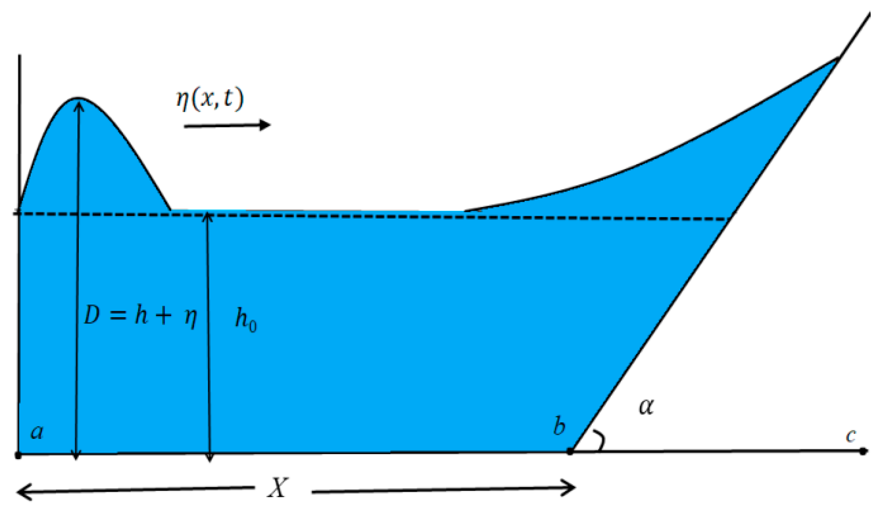
In this simulation, the corresponding bathymetry (Figure 1) set-up is used: the flat part of the flume matches the beach of constant slope:
where h0 is the constant water depth, kept at 3.5 m for all simulations, [a, c] are the left and right boundaries of the numerical flume, [b] is the point where the slope starts, and tan α = 1:6 is the tangent of the bottom slope. For simplicity, the left boundary is taken as (a = 0). The length of the section of constant depth is b = 251.5 m, and the right limit of the numerical flume is taken as c = 291.5 m. The number of spatial grid points along the distance between [a] and [c] is fixed and equal to 1000 for all experiments. The time step is chosen to satisfy the Courant–Friedrichs–Lewy condition for all considered significant wave heights. The spatial grid step is, therefore, 25 cm, which corresponds to 4 cm vertical resolution for runup height. This was done in order to limit simulation time, when running 10,000 h of physical time of wave propagation. However, this also implies that we have a low resolution and not so reliable statistics, especially for small amplitude waves Hs = 0.1 m. In a similar manner to the significant wave height, Hs, the significant runup height, Rs, is introduced as an average of one third of the largest runup heights in the time-series. The significant runup height for this small amplitude case is Rs = 0.23 m, so even in this case, the resolution is low, but considerable.
Of course, the number of extreme runups in this resolution is also somehow underrepresented; however, all qualitative and comparative conclusions of this study still hold on.
Boundary Condition
On the left extremity x = a of the computational domain, the Dirichlet boundary condition on the total water depth component D(a, t) = h0 + η0(t) of the solution (D, Du) is imposed. Namely, the free surface elevation function, η0, is drawn from a narrow- or wide-band Gaussian signal depending on the experiment. These data turn out to be enough to obtain a well-posed initial boundary-value problem provided that the flow is subcritical at the point x = a, i.e., , which is always the case for Riemann waves (see [26] for the rigorous mathematical justification of this fact in case of transparent boundary conditions). The boundary conditions are implemented in the finite volume scheme according to the method described in [27] (see also [28] for more details on the application to the nonlinear shallow water equations).
The considered boundary condition (wave field offshore) is distributed by the Gaussian distribution:
where σ is a standard deviation, and μ is a mean value of the distribution. To ensure this, all individual time-series have been verified by the Kolmogorov-Smirnov test [29].
The spectrum of the generated waves is:
where f is the wave frequency, Δf is the frequency band, f0 = 0.1 Hz is the central frequency, and S0 is the constant, which is calculated in order to achieve the desired Hs.
In this work, the case with Δf/f0 = 0.1 is referred to as the narrow-band spectrum, while the case with Δf/f0 = 0.4 is referred to as the wide-band spectrum. In order to study the influence of wave nonlinearity during wave propagation to the coast, waves of different significant wave heights, which are calculated as the average of one third of the largest wave heights in the time-series (Hs = 0.1, 0.2, 0.3, 0.4, and 0.5 m), are considered. The calculated time-series for each Hs is 1000 h (360,000 wave periods). Parallel computations facilitated the calculation of the statistics of wave runup characteristics for 5000 h, for each bandwidth, and 10,000 h in total. The numerical computations were carried out in MATLAB and run on a cluster containing 28 cores.
The parameter of the nonlinearity for generated waves was estimated as Hs/h0 and changed from 0.03 to 0.14. The characteristic parameter kh0 = 0.38 is at the border of validity of the shallow water theory, taking into account the horizontal extent of the wave tank. The phase velocity relative error committed by non-dispersive theory for kh0 = 0.38 is only 2.3%. Thus, at the end of the numerical wave tank, the difference between wave crest positions (between dispersive and non-dispersive models) is less than 10%. Since the focus of this paper is on wave runup, the choice of this theory is justifiable. The choice of wave parameters allows us to see the effects of wave breaking on the statistics of their runups. The type of wave breaking is defined by the Iribarren number [5]:
where H is the wave height and L is the characteristic wavelength offshore. It is surging or collapsing for Ir ≥ 3.3, plunging for 0.5 ≤ Ir ≤ 3.3, and spilling for Ir ≤ 0.5. In our dataset, only the first two types of wave breaking, surging or collapsing and plunging, are observed. For Hs/h0 = 0.03, less than 1% of waves experience plunging breaking, while most of the waves are surging. With an increase in Hs/h0, the percentage of plunging waves increases. For Hs/h0 = 0.06, 32–35% of the waves are plunging, for Hs/h0 = 0.09, 61–65% of the waves are plunging, for Hs/h0 = 0.11, 71–76% of the waves are plunging, and for the most nonlinear case, Hs/h0 = 0.14, 85–88% of the waves are plunging.
3. Data Analysis and Results
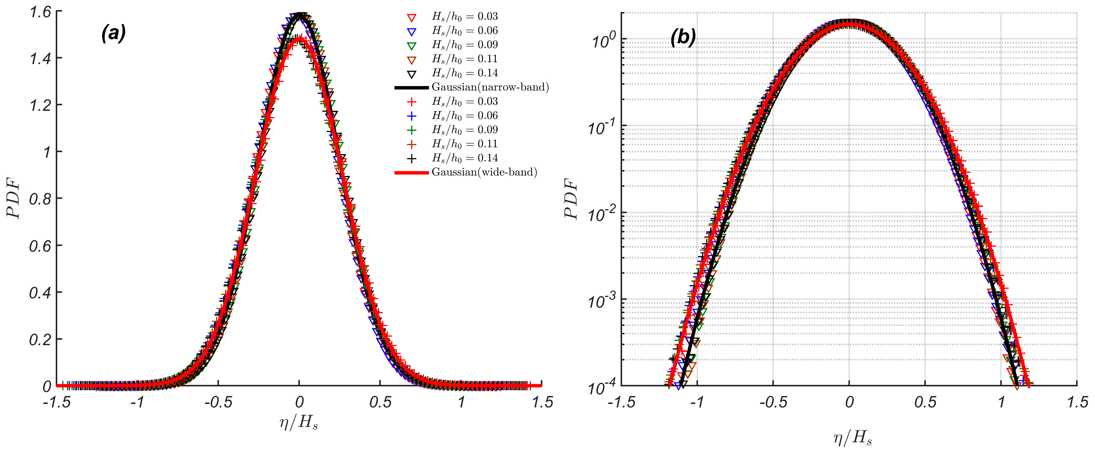
Figure 2 shows probability density functions (PDF) of narrow-band and wide-band wave fields for different nonlinearities, Hs/h0. The data of the narrow-band spectra, Δf/f0 = 0.1 are shown by triangles (different colors correspond to different nonlinearities), while the corresponding Gaussian distribution (µ = 0, σ = 0.25) is shown by the black solid line. The data of the wide-band spectra, Δf/f0 = 0.4 are shown by pluses, and the corresponding Gaussian distribution (µ = 0, σ = 0.27) is shown by the red solid line. It can be seen that the generated waves are well described by the Gaussian distribution, which has zero mean, skewness and kurtosis for all nonlinearities, Hs/h0.
To describe the wave statistics in Figure 2, the Rayleigh distribution, which is well used for this type of problem [5], is applied:
where ξ is a data vector and λ is the scale parameter. For a better fit, a two-parameter Weibull distribution is also considered:
where λ is the scale parameter and k is the shape parameter.
The wave height distributions of both narrow-band and wide-band wave fields are shown in Figure 3. As expected, the narrow-band data are well described by a Rayleigh distribution (λ = 0.5), although a Weibull distribution gives a slightly better fit (λ = 0.74, k = 2.27). The data of wide-band spectra tend to be distributed according to a Weibull distribution (λ = 0.71, k = 2.06).
The waves which are two times higher than the significant wave height (H/Hs ≥ 2) are the so-called freak waves. It can be seen from Figure 3 that the probability of the freak wave occurrence in the initial wave field is higher for narrow-band signals than for wide-band ones.
The calculated significant runup heights Rs for narrow-band and wide-band signals are shown in Figure 4. It is interesting to see that Rs for wide-banded waves is always higher than for narrow-banded waves, which can be explained by the higher variability in wave periods for wide-banded waves. Also, Figure 4 indirectly shows us how many of our waves are breaking. The wave runup height, at which the first wave breaking occurs in the wave trough, can be estimated as Rcr/h0 = g(αT/(2π))2/h0 = 0.2 (see [30] for details). This means that our case of “small” nonlinearity Hs/h0 = 0.03 is affected very little by wave breaking (<1% according to Iribarren criterion). The case of Hs/h0 = 0.06 is affected by wave breaking only for extreme runups (32–35% according to Iribarren criterion). In the case of Hs/h0 = 0.09, more than a half of waves are breaking (61–65% according to Iribarren criterion). However, in the cases of Hs/h0 = 0.11 and Hs/h0 = 0.14, the majority of waves are breaking.
Figure 5 shows the probability distribution functions of runup oscillations, r/Rs for initial Gaussian narrow-banded and wide-banded wave signals. It can be seen from Figure 5a that runup oscillations of narrow-banded waves are no longer distributed by a normal distribution and are slightly shifted to the right towards larger positive values with an increase in nonlinearity. This effect was partially observed both theoretically for an infinite plane beach [11,12] and experimentally [13,14]. What is interesting and peculiar is a strong deformation of the distribution itself. In addition, the tails of these distributions are much thinner than of Gauss, and reflect a relatively weak probability of extreme floods for narrow-banded waves.
The distributions of runup oscillations of the initial wide-band signal are also shifted to the right towards higher runups with an increase in nonlinearity, but this shift is much larger compared to that of the narrow-band signal. Moreover, the tails of these distributions are much thicker than those for narrow-band data, and are rather close to the normal distribution, which corresponds to a relatively large probability of extreme floods for wide-banded waves.
It can also be seen that for both narrow-banded and wide-banded waves, the probability of large waves decreases with an increase in wave nonlinearity, which can be explained by wave breaking.
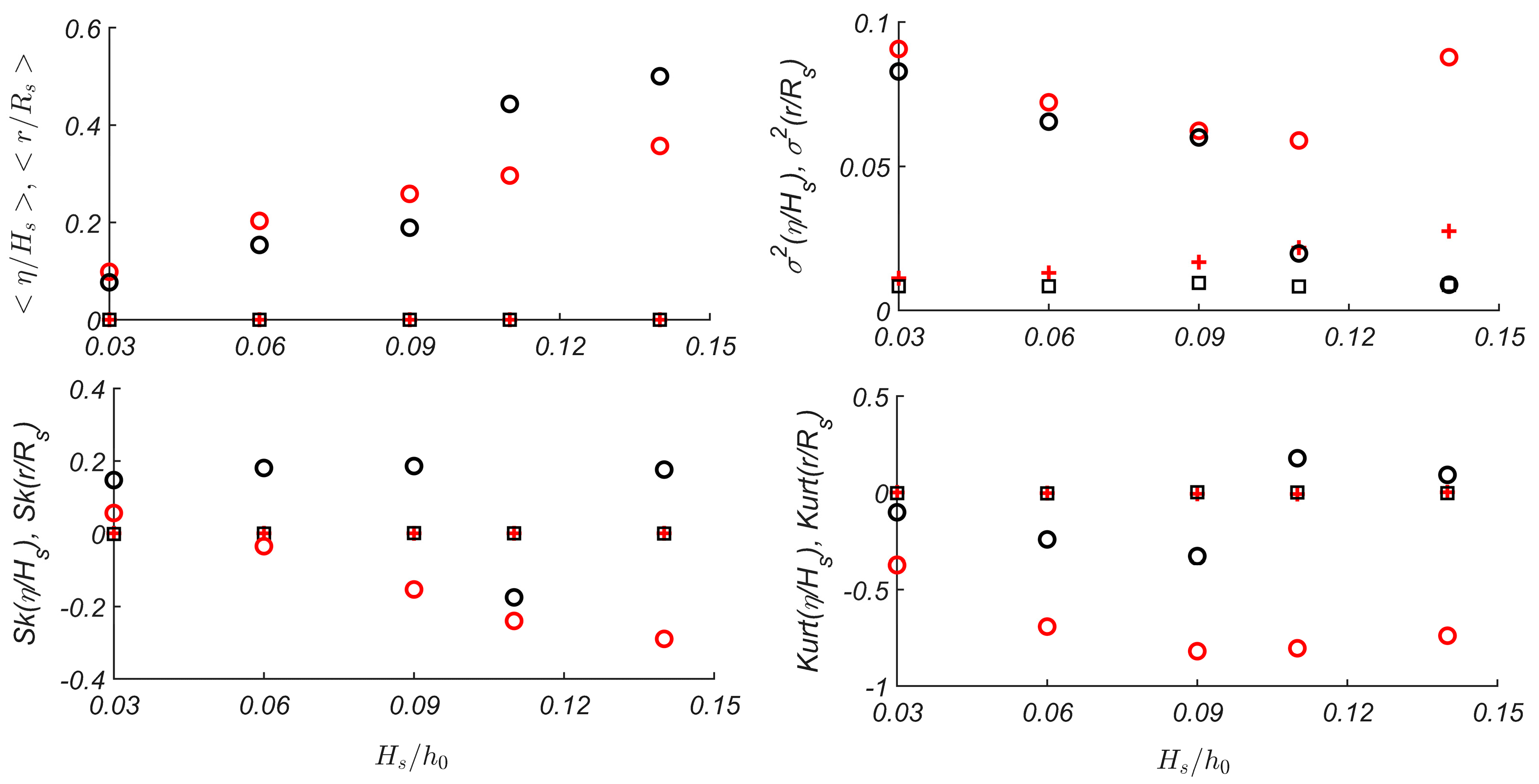
These effects can also be seen in Figure 6, which shows the statistical moments of narrow-banded and wide-banded waves offshore, normalized by Hs, and the corresponding runup oscillations on a beach, normalized by Rs. The statistical moments, mean, variance, skewness, and (normalized) kurtosis are calculated as:
where ξ is a data vector, and n is its length.
Notably, the mean, skewness and kurtosis of both narrow-banded and wide-banded wave fields are zero, providing the desired Gaussian statistics. Regarding runup oscillations, one can see that for both narrow- and wide-banded waves, the mean of runup oscillations rises with the nonlinearity, which reflects the known effect of wave set-up on a beach. For small-amplitude waves, the set-up for narrow-banded waves is larger than for wide-banded ones, while for large amplitude waves, affected by wave breaking, it is the opposite. For wide-banded waves, the variance decreases with an increase in nonlinearity, while for narrow-banded waves it changes non-monotonically. The higher moments, skewness and kurtosis of runup oscillations for waves with a narrow-band spectrum are negative, while for waves with wide-band spectrum they are sign-variable. Also for the narrow-banded waves, the skewness decreases with an increase in wave nonlinearity, while kurtosis changes non-monotonically with an increase in wave nonlinearity. Moreover, for wide-banded waves, both skewness and kurtosis change non-monotonically with an increase in nonlinearity. This somehow only partially corresponds to the theoretical findings in [11], where the kurtosis was positive for weak amplitude waves and negative for strongly nonlinear waves, while the skewness was always positive. However, in the experimental study of [13], the skewness was both positive and negative. It is also important to say that for all four moments, one can see different dynamics for small-amplitude non-breaking or almost non-breaking waves and large-amplitude waves, strongly affected by wave breaking.
Runup oscillations deviate from the Gaussian distribution even for weak-amplitude waves (see Figure 6). With an increase in nonlinearity, all statistical moments of runup oscillations change. It can be seen that statistical moments of narrow-banded irregular waves (except kurtosis) change with Hs monotonically, while for the wide-banded waves, they vary non-monotonically (except mean values).
The large (extreme) wave runup heights, Rextrm = R/Rs ≥ s, where s is some threshold value, somehow behave similarly to a conditional Weibull law whose density is given by Equation (11):
A conditional Weibull law is characterized by three parameters: the shape k, the scale λ and the threshold s. Given the data, (Ri extrm) = 1…n, s is fixed and k and λ are computed by maximum likelihood estimator. The scale parameter, λ can be obtained from Equation (12):
where n is the number of extreme wave runups. In order to obtain the shape parameter, k, one should solve Equation (13):
Similarly to freak waves, the waves on a beach whose runup height is two times larger than the significant runup height (R/Rs ≥ 2) are called freak runups. On gentle beaches, such freak runups are manifested as sudden floods and may result in human injuries and fatalities [8,9,10].
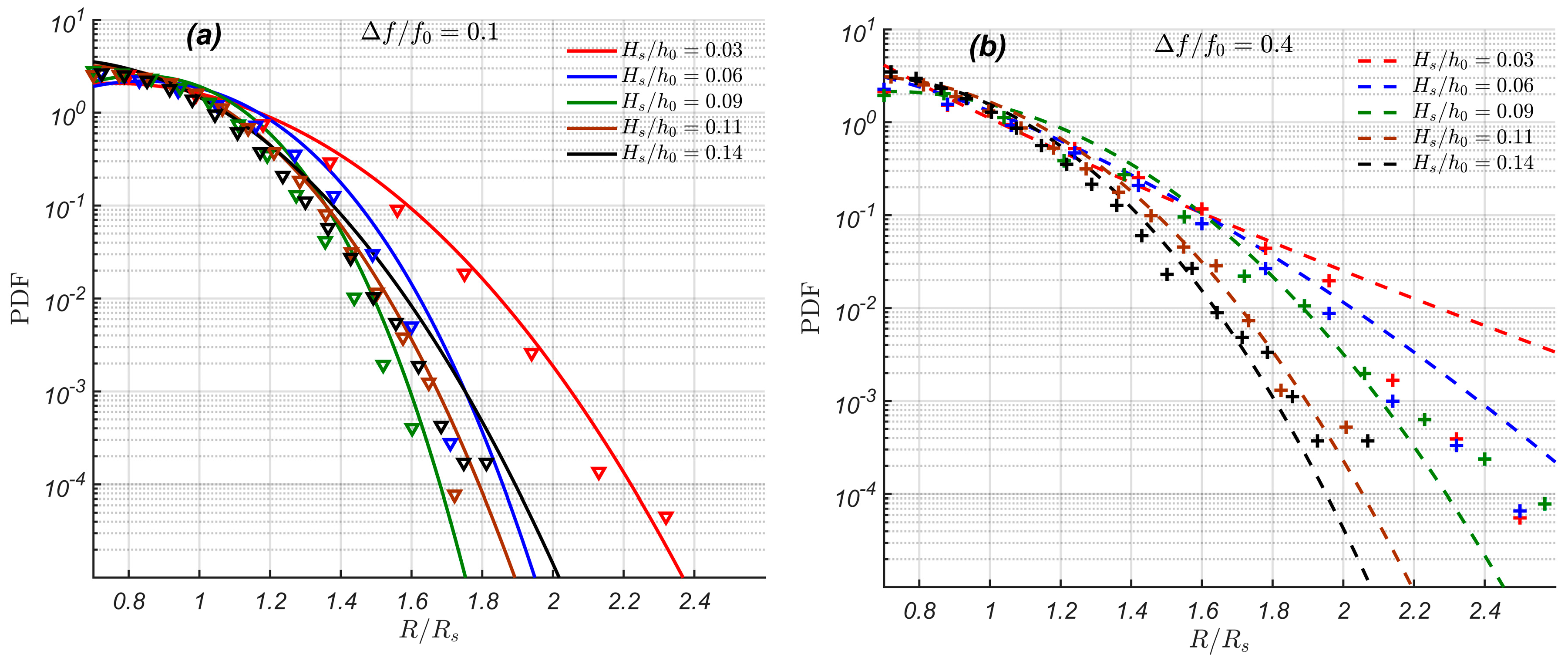
Figure 7 shows probability distribution functions of large runup heights (R ≥ 0.7Rs), for narrow-band and wide-band spectra, for different nonlinearities. It can be seen in Figure 7 that the tails of distributions for runup heights corresponding to freak events for narrow-banded waves decay much faster than those for wave heights offshore (except waves of weak amplitude with Hs/h0 = 0.03), which means that for narrow-banded waves, the probability of freak runup occurrence on a beach is less than the probability of freak wave occurrence in the sea coastal zone, and a gentle beach works as some kind of “filter” for narrow-banded freak events. This is also manifested in the numbers of actual freak events, given in Table 1. It can be seen that for non-breaking waves of the smallest amplitude Hs/h0 = 0.03, the number of freak events on a beach was reduced twice compared to the original number of freak waves offshore, while for waves of larger amplitude, which were affected by the wave breaking, there were no freak runups at all.
In contrast, for wide-banded waves, the probability of freak events on a beach is more or less the same as in the sea coastal zone and may even be higher (Figure 7). The number of freak runups for small non-breaking wide-banded waves increased twice compared to the original number of freak waves offshore (see Table 1). With an increase in wave amplitude (and consequently, wave breaking), the number of freak runups on a beach decreases; however, for waves of moderate amplitude, the number of freak runups is still larger than the number of freak waves offshore, while for waves strongly affected by the wave breaking (Hs/h0 = 0.11 and 0.14), the number of freak runups on a beach suddenly drops down (see Table 1).
Probability of extreme wave runups on a beach is noticeably higher for waves with wide-band spectra than for waves with narrow-band spectra (see Figure 7), although the probability of extreme wave heights in the wave field offshore is significantly higher for narrow-banded waves than for wide-banded ones (see Figure 3, Table 1).
The probability of extreme runup formation changes with the wave nonlinearity. It decreases with an increase in wave nonlinearity for wide-banded waves and changes non-monotonically with nonlinearity for narrow-banded waves. It is also interesting to see that the tails of distributions in Figure 7 are somehow gathered into clusters and can be separated in two groups for “relatively large Hs” and “relatively small Hs”, where the “small Hs” group is always higher than the “large Hs” group. The latter holds for both narrow-banded and wide-banded waves and can be explained by the wave breaking.
The corresponding data of wave runup heights are also approximated by a conditional Weibull distribution (Equation (11)), which gives reasonable results and can be used to evaluate the probability of freak runups. Here, the threshold s is selected as 0.7 and the calculated parameters k and λ are given in Table 2.
4. Conclusions
In this paper, irregular wave runups on a plane beach are studied by means of direct numerical simulations. The numerical model is based on the nonlinear shallow water equations and is of the second order of accuracy. The corresponding bathymetry consists of a section of constant depth, which is matched with the beach of a constant slope. The irregular waves are represented by the Gaussian wave field with spectra of two different bandwidths, which are referred to as narrow-banded and wide-banded waves. To address different levels of wave nonlinearity, time-series with five different significant wave heights are considered. The selected wave regimes represent (i) non-breaking waves, (ii) waves slightly affected by wave breaking, (iii) moderate wave breaking and (iv) significant wave breaking, when the majority of waves are breaking. Each of these time-series has a duration of 1000 h (360,000 wave periods).
The heights of narrow-banded waves are well described by Rayleigh distribution, while heights of wide-banded waves are described by Weibull distribution, irrespective of the wave nonlinearity. However, for wide-banded waves, the tails of these distributions show larger variability than for narrow-banded ones.
As expected, the runup oscillations are not Gaussian, which confirms that results of many previous studies, both theoretical [11,12] and experimental [13,16,17]. For both narrow-band and wide-band cases, one can observe the effect of wave set-up (increase in the mean value of runup oscillations), which increases with an increase in wave nonlinearity. However, for wide-banded waves, this increase is significantly stronger than for narrow-banded ones.
Regarding extreme, so-called “freak events”, their statistics in the initial narrow-banded wave signal offshore are more representative than on the beach (“freak runups”), even for non-breaking waves. Therefore, for narrow-banded waves, gentle beaches reduce the number of freak events as compared to the sea coastal zone, and work as a ‘low-pass filter’ for extreme wave heights. This may explain why freak events on a beach are so unexpected [8,9,10]. However, for wide-banded waves, such an effect has not been observed and the probability of freak events on a beach was similar to or even larger than the one in the sea coastal zone.
The number of freak events in wide-band and narrow-band cases varies, such that increase in the bandwidth leads to a substantial increase in the number of freak events. This can be explained by higher variability in wave periods for wide-banded waves, and wave runup height is rather sensitive to these variations. In addition, the number of freak waves decreases with an increase in wave amplitude and consequently, wave breaking. The largest number of freak waves was observed for non-breaking wide-banded waves, which almost doubled the number of freak waves in the boundary condition wave record.
Finally, to describe statistics of extreme wave runup heights on a gentle beach, a conditional Weibull distribution is suggested. It gives reasonable results and may be used for the assessment of extreme inundations on a beach (freak runups). In addition, in future applications, the statistical analysis hereby provided might also be useful in the study of the wave run-up phenomenon in other applications, e.g., in structures placed in shallow water conditions [31,32].
The limitation imposed by the resolution of the numerical simulations should also be taken into account. Although the number of freak waves on the beach may be somehow reduced by a coarse model resolution, the qualitative and comparative conclusion of this study should not be affected. This point will be improved in our future studies.
Author Contributions
Conceptualization, I.D.; methodology, I.D., D.D., C.L.; software, D.D.; resources, I.D., D.D.; data curation, A.A.; writing—original draft preparation, A.A.; writing—review and editing, A.A., I.D., D.D. and C.L.; numerical simulations and data analysis, A.A.; Conditional Weibull distribution conceptualization and fitting C.L. All authors have read and agreed to the published version of the manuscript.
Funding
The study of distribution functions and the statistical moments of irregular wave runup was performed with the support of an RSF grant (16-17-00041). The numerical simulations of wave runup were supported by an ETAG grant (PUT1378). The authors also thank the PHC PARROT project (No. 37456YM), which funded the visits to France and Estonia, thus facilitating this collaboration.
Acknowledgments
The computations were performed using the computer cluster of the Department of Marine Systems of Tallinn University of Technology.
Conflicts of Interest
The authors declare no conflicts of interest.
References
- Didier, D.; Baudry, J.; Bernatchez, P.; Dumont, D.; Sadegh, M.; Bismuth, E.; Bandet, M.; Dugas, S.; Sévigny, C. Multihazard simulation for coastal flood mapping: Bathtub versus numerical modelling in an open estuary, Eastern Canada. Flood Risk Manag. 2019, 12, 12505. [Google Scholar] [CrossRef]
- Gallien, T.W.; Sanders, B.F.; Flick, R.E. Urban coastal flood prediction: Integrating wave overtopping, flood defenses and drainage. Coast. Eng. 2014, 91, 18–28. [Google Scholar] [CrossRef]
- Beck, M.W.; Losada, I.J.; Menéndez, P.; Reguero, B.G.; Díaz-Simal, P.; Fernández, F. The global flood protection savings provided by coral reefs. Nat. Commun. 2018, 9, 1–9. [Google Scholar] [CrossRef] [PubMed] [Green Version]
- Lyddon, C.E.; Brown, J.M.; Leonardi, N.; Saulter, A.; Plater, A.J. Quantification of the uncertainty in coastal storm hazard predictions due to wave-current interaction and wind forcing. Geophys. Res. Lett. 2019, 46, 14576–14585. [Google Scholar] [CrossRef] [Green Version]
- Massel, R.S. Ocean Surface Waves: Their Physics and Prediction, 2nd ed.; World scientific: Hackensack, NJ, USA, 1996. [Google Scholar]
- Stocker, J.J. Water Waves: The Mathematical Theory with Applications; Interscience: New York, NY, USA, 1957. [Google Scholar]
- Mei, C.C. The Applied Dynamics of Ocean Surface Waves; World Scientific: Singapore, 1983. [Google Scholar]
- Nikolkina, I.; Didenkulova, I. Catalogue of rogue waves reported in media in 2006–2010. Nat. Hazards 2012, 61, 989–1006. [Google Scholar] [CrossRef]
- García, M.G.; Özkan, H.T.; Ruggiero, P.; Holman, R.A.; Nicolini, T. Analysis and catalogue of sneaker waves in the US Pacific Northwest between 2005 and 2017. Nat. Hazards 2018, 94, 583–603. [Google Scholar] [CrossRef]
- Didenkulova, E. Catalogue of rogue waves occurred in the World Ocean from 2011 to 2018 reported by mass media sources. Ocean Coast. Manag. 2020, 188, 105076. [Google Scholar] [CrossRef]
- Didenkulova, I.; Pelinovsky, E.; Sergeeva, A. Statistical characteristics of long waves nearshore. Coast. Eng. 2011, 58, 94–102. [Google Scholar] [CrossRef]
- Gurbatov, S.; Pelinovsky, E. Probabilistic characteristics of narrow-band long-wave run-up onshore. Nat. Hazards Earth Syst. Sci. 2019, 19, 1925–1935. [Google Scholar] [CrossRef] [Green Version]
- Denissenko, P.; Didenkulova, I.; Pelinovsky, E.; Pearson, J. Influence of the nonlinearity on statistical characteristics of long wave runup. Nonlinear Process. Geophys. 2011, 18, 967–975. [Google Scholar] [CrossRef]
- Denissenko, P.; Didenkulova, I.; Rodin, A.; Listak, M.; Pelinovsky, E. Experimental statistics of long wave runup on a plane beach. J. Coast. Res. 2013, 65, 195–200. [Google Scholar] [CrossRef]
- Nielsen, P.; Hanslow, D.J. Wave runup distributions on natural beaches. Coast. Res. 1991, 7, 1139–1152. [Google Scholar]
- Huntley, D.A.; Guza, R.T.; Bowen, A.J. A universal form for shoreline run-up spectra. Geophys. Res. 1977, 82, 2577–2581. [Google Scholar] [CrossRef]
- Hughes, M.G.; Moseley, A.S.; Baldock, T.E. Probability distributions for wave runup on beaches. Coast. Eng. 2010, 57, 575–584. [Google Scholar] [CrossRef]
- Simarro, G.; Bryan, K.R.; Guedes, R.M.; Sancho, A.; Guillen, J.; Coco, G. On the use of variance images for runup and shoreline detection. Coast. Eng. 2015, 99, 136–147. [Google Scholar] [CrossRef]
- Salmon, S.A.; Bryan, K.R.; Coco, G. The use of video systems to measure run-up on beaches. J. Coast. Res. 2007, 50, 211–215. [Google Scholar]
- Aagaard, T.; Holm, J. Digitization of wave run-up using video records. J. Coast. Res. 1989, 5, 547–551. [Google Scholar]
- Khoury, A.; Jarno, A.; Marin, F. Experimental study of runup for sandy beaches under waves and tide. Coast. Eng. 2019, 144, 33–46. [Google Scholar] [CrossRef]
- Park, H.; Cox, D.T. Empirical wave run-up formula for wave, storm surge and berm width. Coast. Eng. 2016, 115, 67–78. [Google Scholar] [CrossRef] [Green Version]
- García-Medina, G.; Özkan-Haller, H.T.; Holman, R.A.; Ruggiero, P. Large runup controls on a gently sloping dissipative beach. J. Geophys. Res. Ocean. 2017, 122, 5998–6010. [Google Scholar] [CrossRef]
- Di Luccio, D.; Benassai, G.; Budillon, G.; Mucerino, L.; Montella, R.; Carratelli, E.P. Wave run-up prediction and observation in a micro-tidal beach. Nat. Hazards Earth Sys. Sci. 2018, 18, 2841–2857. [Google Scholar] [CrossRef] [Green Version]
- Dutykh, D.; Katsaounis, T.; Mitsotakis, D. Finite volume schemes for dispersive wave propagation and runup. Comput. Phys. 2011, 230, 3035–3061. [Google Scholar] [CrossRef] [Green Version]
- Petcu, M.; Temam, R. The one-dimensional shallow water equations with transparent boundary conditions. Math. Methods Appl. Sci. 2013, 36, 1979–1994. [Google Scholar] [CrossRef]
- Ghidaglia, J.M.; Pascal, F. The normal flux method at the boundary for multidimensional finite volume approximations in CFD. Eur. J. Mech. B/Fluids 2005, 24, 1–17. [Google Scholar] [CrossRef]
- Dutykh, D.; Poncet, R.; Dias, F. The VOLNA code for the numerical modeling of tsunami waves: Generation, propagation and inundation. Eur. J. Mech. B/Fluids 2011, 30, 598–615. [Google Scholar] [CrossRef] [Green Version]
- Dodge, Y. Kolmogorov–Smirnov Test; The Concise Encyclopedia of Statistics; Springer: New York, NY, USA, 2008. [Google Scholar]
- Didenkulova, I. New trends in the analytical theory of long sea wave runup. In Applied Wave Mathematics: Selected Topics in Solids, Fluids, and Mathematical Methods; Quak, E., Soomere, T., Eds.; Springer: Berlin/Heidelberg, Germany, 2009; pp. 265–296. [Google Scholar]
- Vanem, E.; Fazeres-Ferradosa, T.; Rosa-Santos, P.; Taveira-Pinto, F. Statistical description and modelling of extreme ocean wave conditions. In Proceedings of the Institution of Civil Engineers-Maritime Engineering; Thomas Telford Ltd.: London, UK, December 2019; Volume 172, pp. 124–132. [Google Scholar]
- Fazeres-Ferradosa, T.; Taveira-Pinto, F.; Vanem, E.; Reis, M.T.; Neves, L.D. Asymmetric copula–based distribution models for met-ocean data in offshore wind engineering applications. Wind Eng. 2018, 42, 304–334. [Google Scholar] [CrossRef] [Green Version]
Figure 1.
Bathymetry sketch of numerical experiment.

Figure 2.
Probability density functions of normalized narrow-band and wide-band wave fields offshore for different nonlinearities, Hs/h0 in linear (a) and logarithmic (b) scales. Solid lines correspond to Gaussian distributions fitted to the corresponding datasets, shown with a red color for wide-band data and with black color for narrow band data.

Figure 3.
Probability density functions of normalized trough-to-crest wave heights of the initial narrow-band (a) and (c), and wide-band (b) and (d) wave fields for different nonlinearities, Hs/h0 in linear (top) and logarithmic (bottom) scales. The red solid line corresponds to the Rayleigh distribution; the black solid line corresponds to the Weibull distribution fitted to the corresponding dataset.

Figure 4.
Significant runup height, Rs for wide-band (red circles) and narrow-band (black crosses) signals for different nonlinearities.
Figure 4.
Significant runup height, Rs for wide-band (red circles) and narrow-band (black crosses) signals for different nonlinearities.

Figure 5.
Probability density functions of runup oscillations, normalized by a significant runup height, Rs, for different nonlinearities for narrow-banded (a) and (c), and wide-banded (b) and (d) waves in linear (top) and logarithmic (bottom) scales. Solid lines correspond to Gaussian distributions, fitted to the corresponding datasets, using the matching colors.

Figure 6.
Statistical moments of runup oscillations (normalized by Rs) of narrow-banded (red circles) and wide-banded (black circles) waves on a beach, r, versus nonlinearity, Hs/h0. Statistical moments of narrow-band and wide-band wave fields offshore (normalized by Hs) are shown by red crosses and black squares, respectively.

Figure 7.
Probability density functions of large runup heights (R ≥ 0.7Rs) for (a) narrow-banded (triangles) and (b) wide-banded (pluses) waves. Lines correspond to conditional Weibull distributions (Equation (11)), fitted to the narrow-band (solid lines) and wide-band (dashed lines) datasets, using the matching colors.


Table 1.
The number of freak events in the sea coastal zone and on a beach for different wave regimes.
Table 1.
The number of freak events in the sea coastal zone and on a beach for different wave regimes.
| Δf/f0 = 0.1 | Δf/f0 = 0.4 | |||||
|---|---|---|---|---|---|---|
| Hs/h0 | Number of Waves | Freak Waves Offshore | Freak Runups | Number of Waves | Freak Waves Offshore | Freak Runups |
| 0.03 | 362255 | 125 | 61 | 389232 | 51 | 118 |
| 0.06 | 362380 | 117 | 0 | 389385 | 45 | 76 |
| 0.09 | 362096 | 89 | 0 | 389444 | 49 | 62 |
| 0.11 | 362319 | 88 | 0 | 389263 | 53 | 2 |
| 0.14 | 362302 | 102 | 0 | 389728 | 34 | 1 |
Table 2.
Parameters of conditional Weibull distribution fitted to the corresponding datasets in Figure 7.
Table 2.
Parameters of conditional Weibull distribution fitted to the corresponding datasets in Figure 7.
| Δf/f0 = 0.1 | Δf/f0 = 0.4 | |||
|---|---|---|---|---|
| Hs/h0 | k | λ | k | λ |
| 0.03 | 2.747 | 0.886 | 0.76 | 0.116 |
| 0.06 | 3.6 | 0.92 | 1.43 | 0.48 |
| 0.09 | 4.06 | 0.89 | 2.58 | 0.86 |
| 0.11 | 3.08 | 0.777 | 2.6 | 0.772 |
| 0.14 | 3.08 | 0.72 | 2.718 | 0.762 |
© 2020 by the authors. Licensee MDPI, Basel, Switzerland. This article is an open access article distributed under the terms and conditions of the Creative Commons Attribution (CC BY) license (http://creativecommons.org/licenses/by/4.0/).
Share and Cite
MDPI and ACS Style
Abdalazeez, A.; Didenkulova, I.; Dutykh, D.; Labart, C. Extreme Inundation Statistics on a Composite Beach. Water 2020, 12, 1573. https://doi.org/10.3390/w12061573
AMA Style
Abdalazeez A, Didenkulova I, Dutykh D, Labart C. Extreme Inundation Statistics on a Composite Beach. Water. 2020; 12(6):1573. https://doi.org/10.3390/w12061573
Chicago/Turabian StyleAbdalazeez, Ahmed, Ira Didenkulova, Denys Dutykh, and Céline Labart. 2020. "Extreme Inundation Statistics on a Composite Beach" Water 12, no. 6: 1573. https://doi.org/10.3390/w12061573
Note that from the first issue of 2016, this journal uses article numbers instead of page numbers. See further details here.