Regional Inundation Forecasting Using Machine Learning Techniques with the Internet of Things

Abstract

Natural disasters have tended to increase and become more severe over the last decades. A preparation measure to cope with future floods is flood forecasting in each particular area for warning involved persons and resulting in the reduction of damage. Machine learning (ML) techniques have a great capability to model the nonlinear dynamic feature in hydrological processes, such as flood forecasts. Internet of Things (IoT) sensors are useful for carrying out the monitoring of natural environments. This study proposes a machine learning-based flood forecast model to predict average regional flood inundation depth in the Erren River basin in south Taiwan and to input the IoT sensor data into the ML model as input factors so that the model can be continuously revised and the forecasts can be closer to the current situation. The results show that adding IoT sensor data as input factors can reduce the model error, especially for those of high-flood-depth conditions, where their underestimations are significantly mitigated. Thus, the ML model can be on-line adjusted, and its forecasts can be visually assessed by using the IoT sensors’ inundation levels, so that the model’s accuracy and applicability in multi-step-ahead flood inundation forecasts are promoted.

1. Introduction

Flood is one of the most disruptive natural hazards, which causes significant damage to life, agriculture, and economy, and has a great impact on city development. Nowadays, flood tends to increase and become more severe as climate changes together with the rapid urbanization and aging infrastructure in cities. Early notification of flood incidents could benefit the authorities and public for devising preventive measures, preparing evacuation missions, and alleviating flood victims. A precautionary measure to cope with the upcoming flood is flood forecasting and warning involved persons, which would result in the reduction of damage and life lost. Flood forecast models have been developed over the last decades. Among them, physically based models have been commonly used and showed great capabilities for flood estimation, while they often require hydro-geomorphological monitoring datasets and intensive computation, which prohibits short-term prediction [1,2,3]. Statistical models, such as the multiple linear regression (MLR) [4,5,6] and autoregressive integrated moving average (ARIMA) [7,8,9,10] are also frequently used for flood modeling. Nevertheless, their capability for short-term forecasting has been restricted because of the nonlinear dynamic feature of storm events resulting in a lack of accuracy and robustness of the statistical methods [11].

Machine learning (ML) models have a great capability to model the nonlinear dynamic feature and have widely been used in hydrological issues, such as predicting the level of sewage in sewers [12]; arsenic concentration in groundwater [13]; or flood level prediction [14,15,16,17,18,19]. Among the ML models, nonlinear autoregressive models with exogenous inputs (NARX) [20] can adaptively learn complex flood systems and have been reported as valid for flood forecasting [21,22,23,24,25,26]. There is also relevant literature that applied it to regional flood forecasting. For instance, Shen and Chang [27] established a NARX model for flood forecasting in flood-prone areas in Yilan County, Taiwan and demonstrated that it has an error tolerance rate and can effectively suppress error accumulation in predicting the next 1–6 h; and Chang et al. [28,29] proposed the use of self-organizing map combing with recurrent nonlinear autoregressive with exogenous inputs (SOM-RNARX) for multi-time regional flood forecasting model and indicated the method could effectively model regional flood forecasting. It can provide the accuracy and reliability of the flood management system. The majority of these ML models have used rainfall as an input to make regional flood inundation forecasts. A drawback of these models was that they mainly relied on measurements from rain stations, which hinders the models from being sequentially adjusted due to lack of real observed inundation depth. Consequently, most existing models could not properly respond to a sudden flood and could not verify the resultant flood forecasts. Furthermore, the forecast was made based on present data that restrict it from determining flood inundation depths much further ahead. Consequently, there is a research gap from the perspective of ML modeling and the data monitoring system. In light of this, an analysis was conducted on the use of monitoring inundation depth data gathered from urban areas to forecast flooding with a view of on-line updating the model and mitigating the residuals between model outputs and real observed inundation depths.

Internet of Things (IoT) sensors are a useful means of carrying out the monitoring of rivers and other natural environments. They have attractive features: simple to install, low energy consumption, and high-precision sensors. The integration of a large number of IoT sensors can provide on-line comprehensive and broader information to effectively perform environmental monitoring and forecasting [30,31,32,33,34]. Recently, several studies have implemented IoT and big data [35,36,37,38] for flood forecasting. For instance, Chang et al. [39] proposed building an intelligent hydro-informatics integration platform to integrate ML models with sensors data for flood prediction. Sood et al. [40] proposed the Internet of Things (IoT) smart flood monitoring to predict floods and flood levels. Mishra et al. [41] combined IoT and deep learning to identify ditch or drainage channel blockage images. IoT has become one of the vital development projects in Taiwan lately. The authorities’ IoT centers, (e.g., Water Resources Agency) can analyze the data and provide suitable countermeasures and rapidly transmit the data to regional control centers against flood. The integration and application of various sensors can offer a large amount of real-time monitoring data (e.g., inundation depths) for ML models’ updating and testing.

This study intends to use the IoT sensor data to construct a machine learning-based embedded flood forecast model for predicting average flood depth in a river basin. The IoT sensor data will be sequentially fused into the ML model as extra input factors, so that the forecast model can be continuously updated and assessed, and the results can be closer to the current situation. This paper is organized as follows. The next section describes the proposed methodology. Subsequently, Section 3 and Section 4 present the study area and practices relating to flood forecasting systems, respectively. Then, the results of visual assessments and numerical evaluations on studied areas are reported and discussed. Concluding remarks are given in the last section.

2. Methodology

We propose a methodology that couples machine learning models, i.e., the recurrent nonlinear autoregressive with exogenous inputs (RNARX) model [20], with the IoT sensor data for providing multi-step-ahead average regional inundated depth (ARID) during storm events. Various IoT sensor data were explored and implemented into the ML model as input factors to continuously update the model’s parameters for better forecasting the ARID.

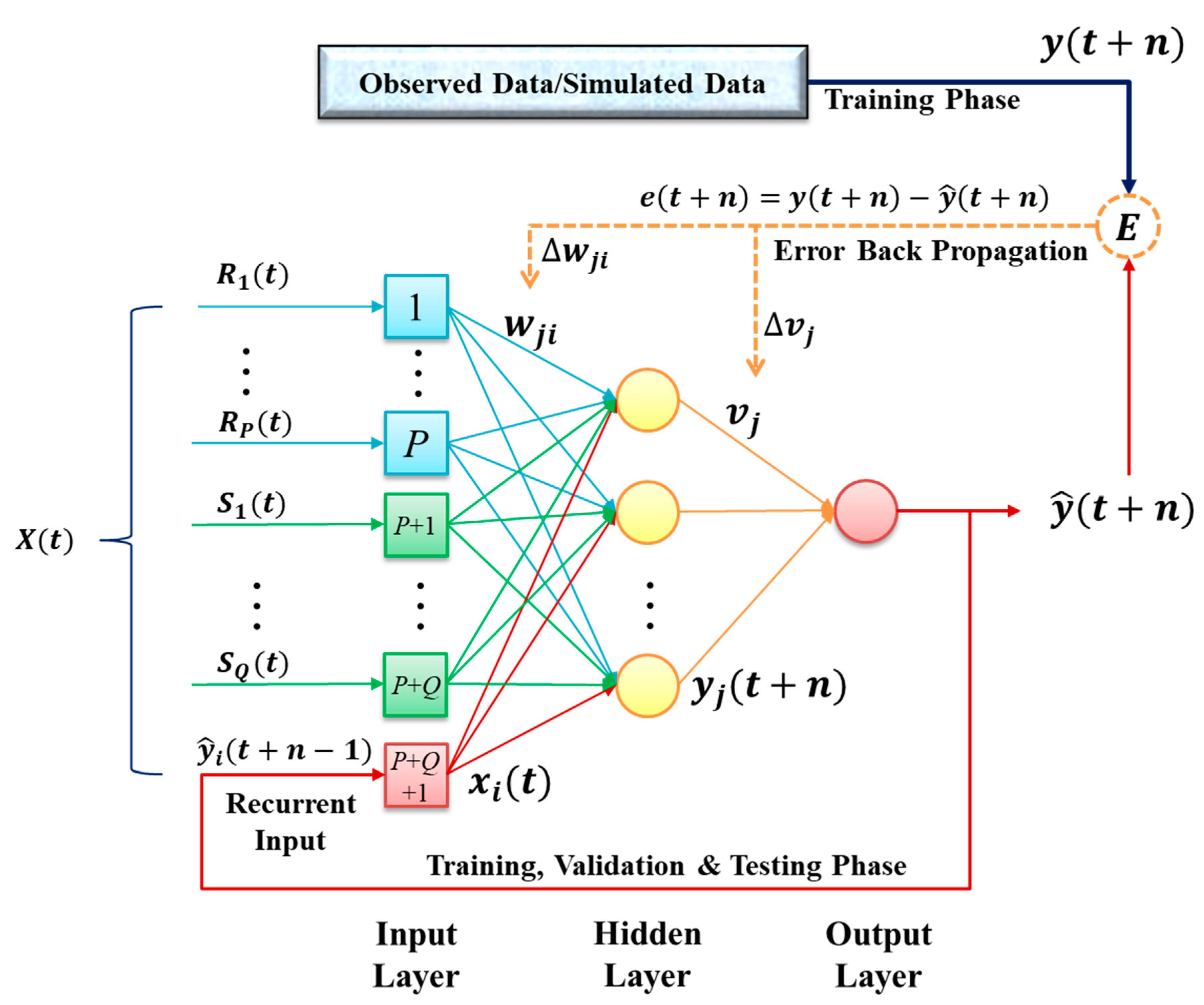
The architecture of the RNARX shown in Figure 1 is a three-layer dynamic neural network. The network was configured by using the model’s outputs as parts of inputs, and its weights can be adjusted by using the conjugate gradient back-propagation learning algorithm. The major difference between the dynamic neural networks (e.g., RNARX) and the static neural networks (e.g., back propagation neural network, BPNN) is that dynamic neural networks use the network output of the current moment as one of the input factors for the next moment, so the model can effectively track the time-series features. The dynamic neural networks have been widely used in modeling time series, especially when there is no actual (observed) value of upcoming time, such as inundation depth. For instance, in this study, the average regional flood inundation depth in the urban area would be continuously predicted along the storm event, while there is no observed value in the coming hours. In model configuring stage, we used simulation results to train and validate the constructed model, while in actual applications, the average flooding depth of all grids, however, cannot be obtained. As known, the longer the forecast horizon, the greater the forecast error would be due to a lack of real monitoring of the inundation depth. In this study, a number of flood sensors implemented in the study area were explored for their effectiveness in modeling the multi-step flood inundation forecasts.

The network contained P rainfall inputs (R), Q flood sensor inputs (S), and one recurrent input from the previous output. Let $X\left(t\right)$ denote the $\left(\mathrm{P}+\mathrm{Q}+1\right)\times 1$ input vector, $\widehat{y}\left(t+n\right)$ denote the n-step-ahead network output, and $y_j\left(t+n\right)$ denote the output vector of the $j\mathrm{th}$ layer. The network multiplied the input factors by weights and forwarded them to the next neuron. The neurons were summed up and outputted through the activation function f (∙), which was continuously forwarded to the final output layer. The output values of each neuron were defined as Equations (1)–(4).

$$ne{t}_j\left(t+n\right)={\displaystyle \sum }_i{w}_{ji}{x}_i\left(t\right)$$

(1)

$$y_j\left(t+n\right)=f\left(ne{t}_j\left(t+n\right)\right)$$

(2)

$$net\left(t+n\right)={\displaystyle \sum }_j{v}_j{y}_j\left(t+n\right)$$

(3)

$$\widehat{y}\left(t+n\right)=f\left(net\left(t+n\right)\right)$$

(4)

Let $W$ denote the $\mathrm{N}\times \left(\mathrm{P}+\mathrm{Q}+1\right)$ weight matrix of the hidden layer. Let $V$ denote the $\mathrm{N}\times 1$ weight matrix of the output layer. RNARX uses the conjugate gradient back-propagation learning algorithm to adjust the average regional inundation depth (ARID) in a specific time during the training phase. The target output value at time t + n and its error vector were defined as $e\left(t+n\right)$, as shown in Equation (5), and the instantaneous error function $E\left(t+n\right)$ was as in Equation (6).

$$e\left(t+n\right)=y\left(t+n\right)-\widehat{y}\left(t+n\right)$$

(5)

$$E\left(t+n\right)=\frac{1}{2}{e}^2\left(t+n\right)$$

(6)

The correction of $v_j$ was defined as the partial differential of the error function $E\left(t+n\right)$ as Equation (7). After the chain-rule process, Equation (8) could be obtained, so $v_j$ was updated in Equations (9) and (10).

$$\frac{\partial E\left(t+n\right)}{\partial v_j}=\frac{\partial \left(\frac{1}{2}{e}^2\left(t+n\right)\right)}{\partial v_j}$$

(7)

$$\begin{gathered} \frac{\partial E\left(t+n\right)}{\partial v_j}=\left(y\left(t+n\right)-\widehat{y}\left(t+n\right)\right)(-f\prime \left(net\left(t+n\right)\right) \\ \times \left(y_j\left(t+n\right)+{\displaystyle \sum }_j{v}_j\left(f\prime \left(ne{t}_j\left(t+n\right)\right)w_{ji}\frac{\partial \widehat{y}\left(t+n-1\right)}{\partial v_j}\right)\right) \end{gathered}$$

(8)

$$\Delta v_j=-{\eta }_2\frac{\partial E\left(t+n\right)}{\partial v_j}$$

(9)

$$v_j\left(p\right)=v_j\left(p-1\right)+\Delta v_j p=epochs$$

(10)

where ${\eta }_2$ is the learning rate. Similarly, we could partially differentiate $w_{ji}$ of the $E\left(t+n\right)$, and the results are shown in Equations (11)–(14).

$$\frac{\partial E\left(t+n\right)}{\partial w_{ji}}=\frac{\partial \left(\frac{1}{2}{e}^2\left(t+n\right)\right)}{\partial w_{ji}}$$

(11)

$$\begin{gathered} \frac{\partial E\left(t+n\right)}{\partial w_{ji}}=\left(y\left(t+n\right)- \widehat{\mathrm{y}}\left(t+n\right)\right)(-f\prime \left(net\left(t+n\right)\right) \\ \times \left({\displaystyle \sum }_j{v}_j{f}^{\prime }\left(ne{t}_j\left(t+1\right)\right)\left(w_{ji}\frac{\partial \left(\widehat{y}\left(t+n-1\right)\right)}{\partial w_{ji}}+{\delta }_{ji}{x}_i\left(t\right)\right)\right) \end{gathered}$$

(12)

$$\Delta w_{ji}=-{\eta }_1\frac{\partial E\left(t+n\right)}{\partial w_{ji}}$$

(13)

$$w_{ji}\left(p\right)=w_{ji}\left(p-1\right)+\Delta w_{ji} p=epochs$$

(14)

where ${\eta }_1$ is the learning rate; ${\delta }_{ji}$ is Kronecker delta with value 1 if and only if $i=j$. Through the above weight adjusting process, the error, because of the complicated interaction between the inputs (rainfall, sensor data, feedback flood depth) and the outputs (flood depth at time T + 1–T + 3), would be computed, and the weights were systematically adjusted through continuous iterations so that the error would be gradually reduced until the satisfactory accuracy and/or the number of iterations was reached for the set requirements. Therefore, the RNARX model was used to predict the multi-step-ahead flood depth, and at the same time, the differences by using only rainfall and the extra sensors of inundation were compared.

3. Study Area and Datasets

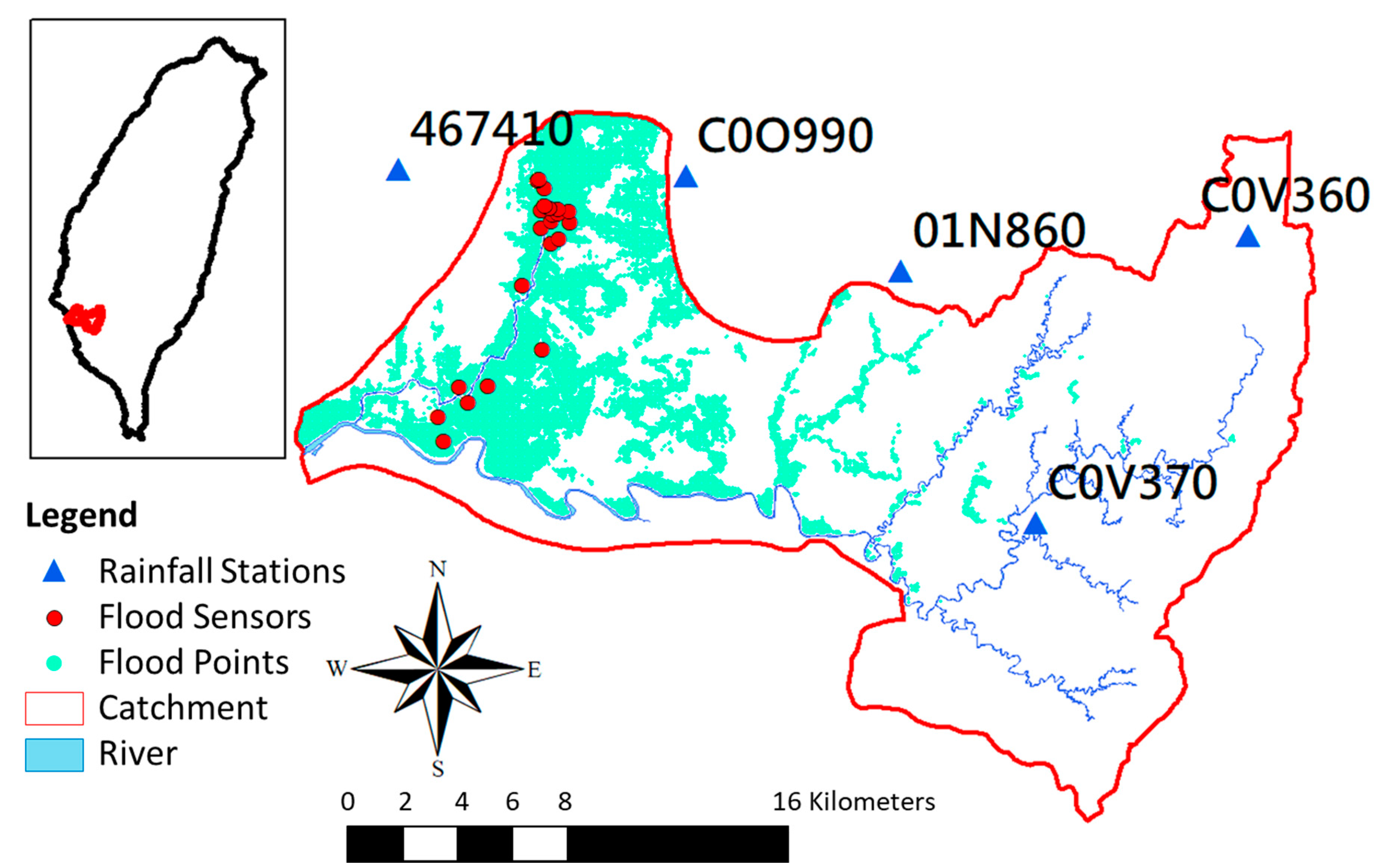
This research area was the Erren River basin (Figure 2) located in southern Taiwan. The river length is 63.2 km with the upstream up to 460 m above sea level, and the catchment area is 350.4 km², which is further divided into 10,744 grids (40 m × 40 m). In this study, six actual storm events and twelve designed rainfall patterns with various return periods, as well as their correspondent 2D flood simulation results (simulated by the SOBEK software of Deltares), were collected from the Water Resources Agency. A total of 631 hourly datasets were used to configure the ML models. There were also 631 regional flood inundation maps generated by the SOBEK based on the rainfall patterns mentioned above, which were used as the virtual inundation maps for ML models’ training and testing. These datasets were further divided into 391 datasets (10 events) for training, 144 datasets (4 events) for validation, and 96 datasets (4 events) for testing (

Table 1. Simulation events used for model training, validation, and testing.

Event Number	Event Name	Average Rainfall (mm/h)	Total Rainfall (mm)	Average Inundation (m)	Max Inundation (m)
Training phase (number of data: 391 h)
1	24H800 mm1	33.3	800	0.46	0.89
2	24H450 mm	18.8	450.1	0.17	0.34
3	24H200 mm	8.3	200	0.05	0.10
4	24H10 y	17.4	417.6	0.14	0.32
5	24H500 y2	33.5	803.7	0.49	0.91
6	201907193	3.2	99.7	0.01	0.02
7	20170601	1.2	86.7	0.01	0.02
8	20160925	7.6	550.1	0.16	0.34
9	20160912	2.7	128.7	0.03	0.10
10	20190813	4.7	226.2	0.07	0.20
Validation phase (number of data: 144 h)
11	24H50 y	24.1	578	0.22	0.43
12	24H400 mm	16.7	400	0.16	0.29
13	24H5 y	14.4	344.8	0.11	0.27
14	20170613	1.4	100.2	0.01	0.03
Testing phase (number of data: 96 h)
15	24H100 y	26.9	646.1	0.26	0.52
16	24H2 y	9.8	234.7	0.06	0.11
17	24H500 mm	20.9	500.5	0.17	0.34
18	24H300 mm	12.5	300	0.11	0.25

^1,2 24H800 mm and 24H500 y are the design storm events of 800 mm and 500-year for 24 h rainfall, respectively. ³ 20190719 (i.e., 2019, 07, 19) means the real event happened on the 19 July 2019.

).

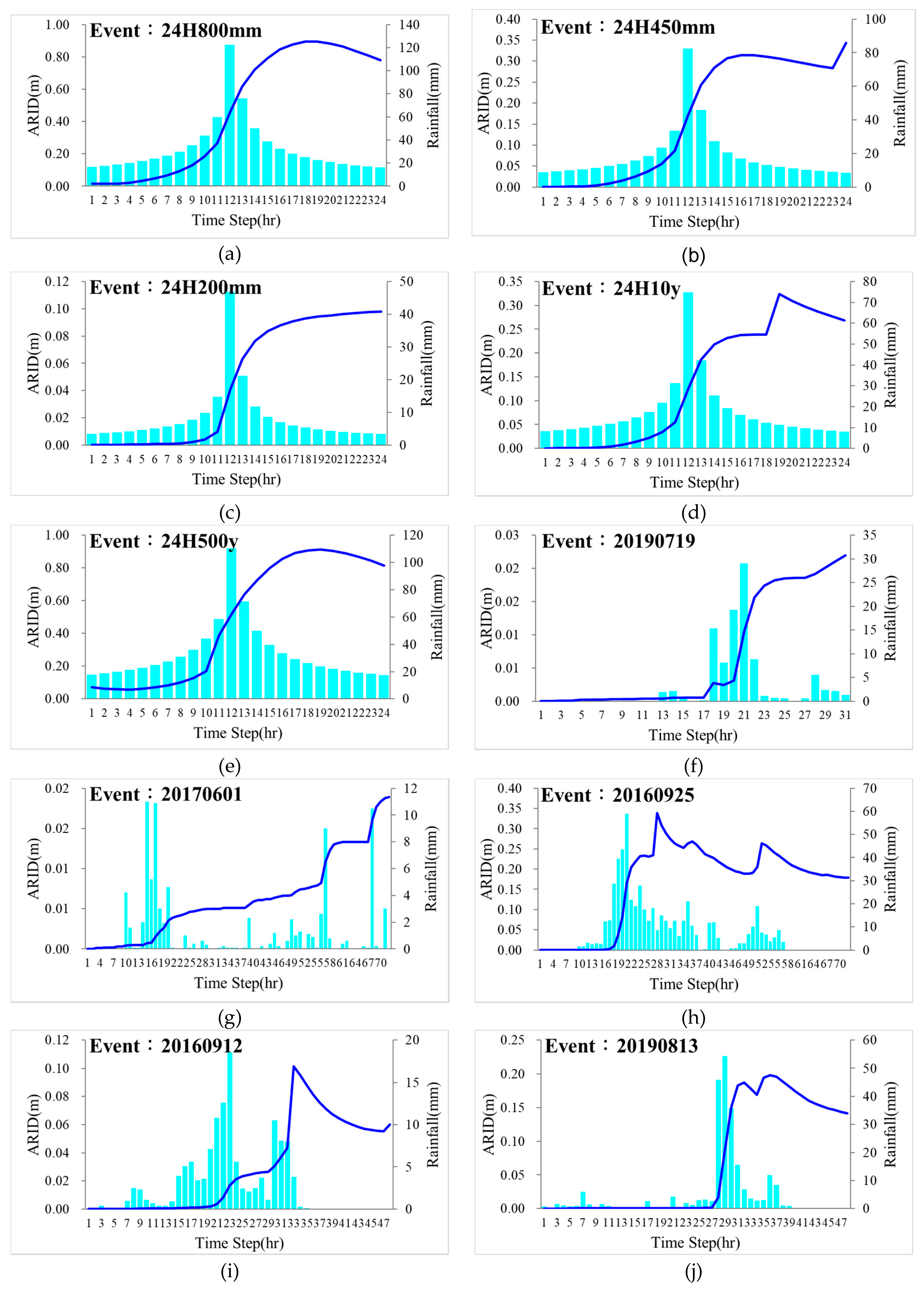
Figure 3 shows a graph of rainfall and average regional flooding depth (ARID) history of 10 training events, which included three quantitative rainfalls (200, 450, and 800 mm), two different return period rainfalls (10 and 500 years), and five actual rainfall events. The rainfall pattern of quantitative rainfalls and two return period rainfalls adopted the centrally concentrated rain pattern, where the maximum rainfall is placed in the center and then sorted according to the amount of rainfall to the right and left, respectively. The average regional inundation depth (ARID) in a specific time was calculated by summarizing all the inundation depths in each grid and then dividing by the number of grids. The time series of ARID shown in Figure 3 presents a complete hydrograph for the correspondent rainfall event (pattern), with the ARID value along with the time from rising limb to the peak and then to the recession limb. We noticed that the actual rainfall events show more irregular rainfall patterns and produce a variant ARID hydrograph. According to the design of training cases, the model can learn the relationship between the different magnitudes of rainfall (large or small) and rainfall types (design rainfall or actual rainfall) with their correspondent average flooding depths during the training process.

4. Model Construction

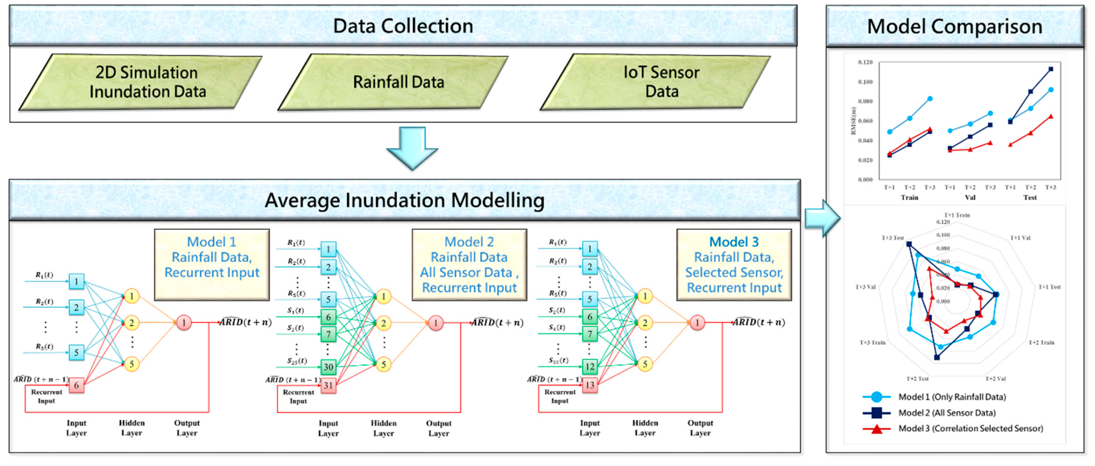
The research process was divided into three stages as shown in Figure 4. The first stage was to collect data, which includes two-dimensional flood simulation data, five stations of rainfall data, and 25 stations of flood sensor datasets. The total datasets were divided into three independent datasets for model training, validation, and testing. The second stage was to construct the forecast models. Three models were built to make multi-step-ahead forecasts of the average regional inundation depth (ARID). The models’ parameters are shown in

Table 2. Parameters of the proposed models.

Parameters	Model 1	Model 2	Model 3
Input	1. Rainfall Data 2. Recurrent Model Output	1. Rainfall Data 2. All Sensor Data 3. Recurrent Model Output	1. Rainfall Data 2. Correlation Selected Sensor 3. Recurrent Model Output
Input Dimension Counts	Rainfall = 5 Sensor = 0 Recurrent = 1	Rainfall = 5 Sensor = 25 Recurrent = 1	Rainfall = 5 Sensor = 7 Recurrent = 1
Hidden Neuron Counts	5	5	5
Weights Counts	41	166	76

. The input factors of Model 1 were 5 rainfall stations’ data ($R_1~R_5$) and one model’s self-feedback value $\widehat{ARID}\left(t+n-1\right)$, a total of 6 input factors, and the number of weights was 41. Model 2 used 5 rainfall stations’ data ($R_1~R_5$), 25 flood sensors’ data ($S_{01}~S_{25}$), and one model’s self-feedback value $\widehat{ARID}\left(t+n-1\right)$, a total of 31 input factors, the number of weights was 166. Model 3 used 5 rainfall stations’ data ($R_1~R_5$), 7 stations of flood representative sensor data ($\mathrm{i}.\mathrm{e}., S_{02},S_{04},S_{05},S_{09},S_{13},S_{15},S_{22}$) selected through correlation analysis, and one model’s feedback value $\widehat{ARID}\left(t+n-1\right)$, a total of 13 input factors, the number of weights was 76. The third stage was to assess the results of the three models using evaluation indicators.

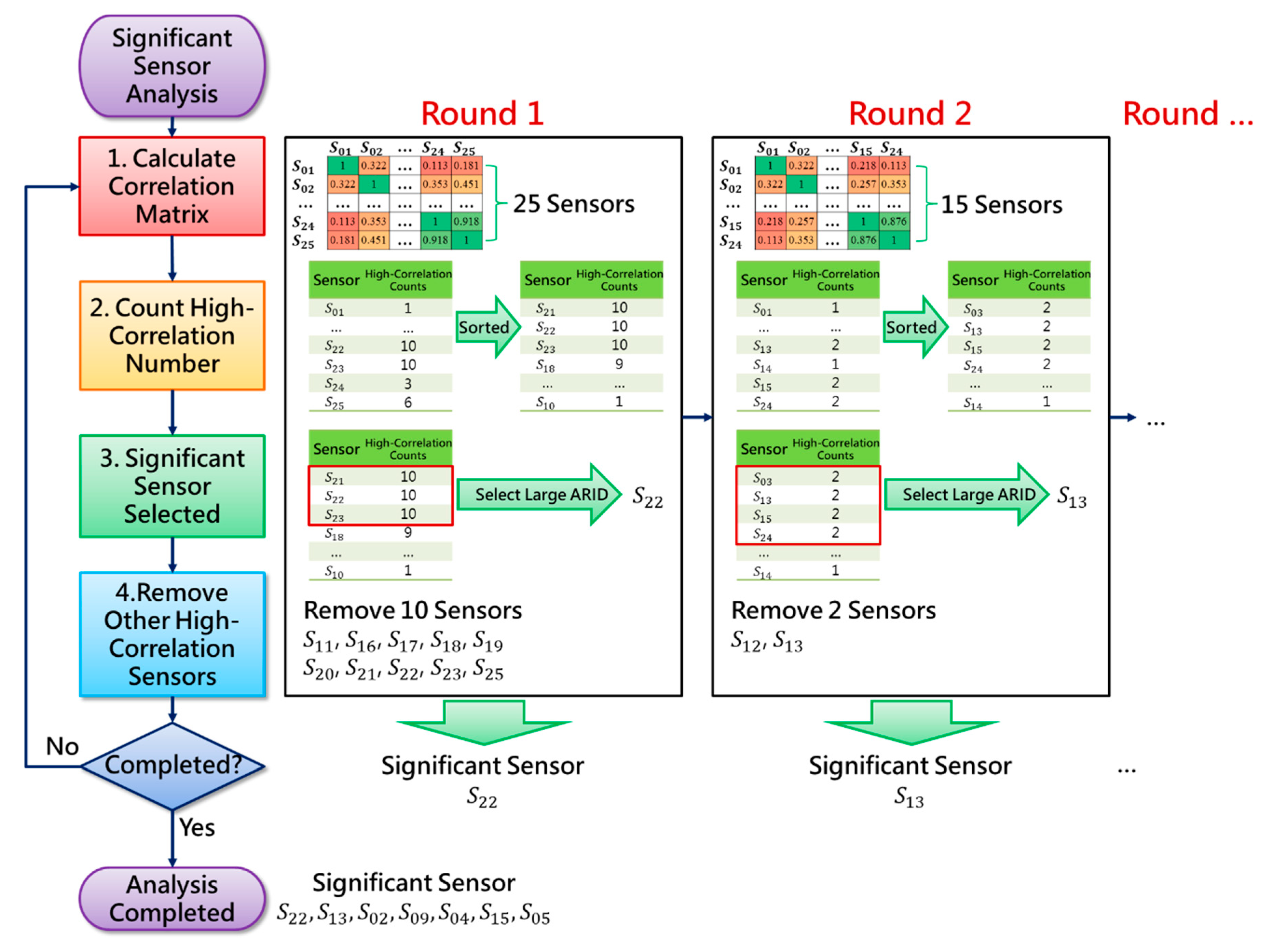
Input variable selection is an essential step in the development of machine learning models. In recent years, various input selection methods have been satisfactorily used to improve prediction accuracy and produce parsimonious models in numerous applications [42,43,44,45]. For instance, in hydrological issues, Taormina and Chau [46] used binary-coded particle swarm optimization and extreme learning machines for rainfall–runoff modeling; Chang et al. used the Gamma test to identify the most suitable input variables for multi-step-ahead water level forecasting [26] and estimating stream total phosphate concentration [47]. While new methods continue to emerge, each has its own advantages and limitations, and there is no best method for all modeling purposes. In this study, we aimed learn whether the new implemented 25 sensors in the study area could be beneficial to model the regional flood inundation forecast. The input variable selection was mainly based on correlation analysis between the sensors. As shown above, the main difference between Model 2 and Model 3 was that Model 2 used all sensors (25) as the model input, while Model 3 used 7 selected sensors as input. A 25 × 25 correlation matrix was constructed. The selection process is shown in Figure 5 and explained as follows.

• Calculate the correlation matrix between sensors.
• Count the number of highly correlated (R² > 0.9) sensors and sorting their number from large to small.
• Select a representative sensor from those sensors that have the highest number of correlated sensors; if the number is the same, compare their ARID and then select the sensor with the largest ARID for priority selection (as the representative sensor).
• Remove those highly correlated sensors with the above representative sensor to avoid repeated selection. For example, in the first round, $S_{22}$ was selected as the representative sensor (Figure 5). Before moving to the next round of selection, those sensors highly correlated with $S_{22}$ sensor (i.e., R² > 0.9) would be removed from the correlation matrix. In this round, 10 sensors (including $S_{22}$) were removed.
• If the selection has not been completed, return to step 1 and recalculate the correlation matrix of the remaining sensors until the selection is completed. That is, all the sensors will either be selected as the representative sensors or be removed during the selection process.

In this way, one of the most representative sensors will be selected for each round until all sensors have been picked or removed. We noticed that this study conducted a total of 7 rounds and picked out ${\mathrm{S}}_{22},{\mathrm{S}}_{13},{\mathrm{S}}_{02},{\mathrm{S}}_{09},{\mathrm{S}}_{04},{\mathrm{S}}_{15},{\mathrm{S}}_{05}$, a total of 7 representative sensors.

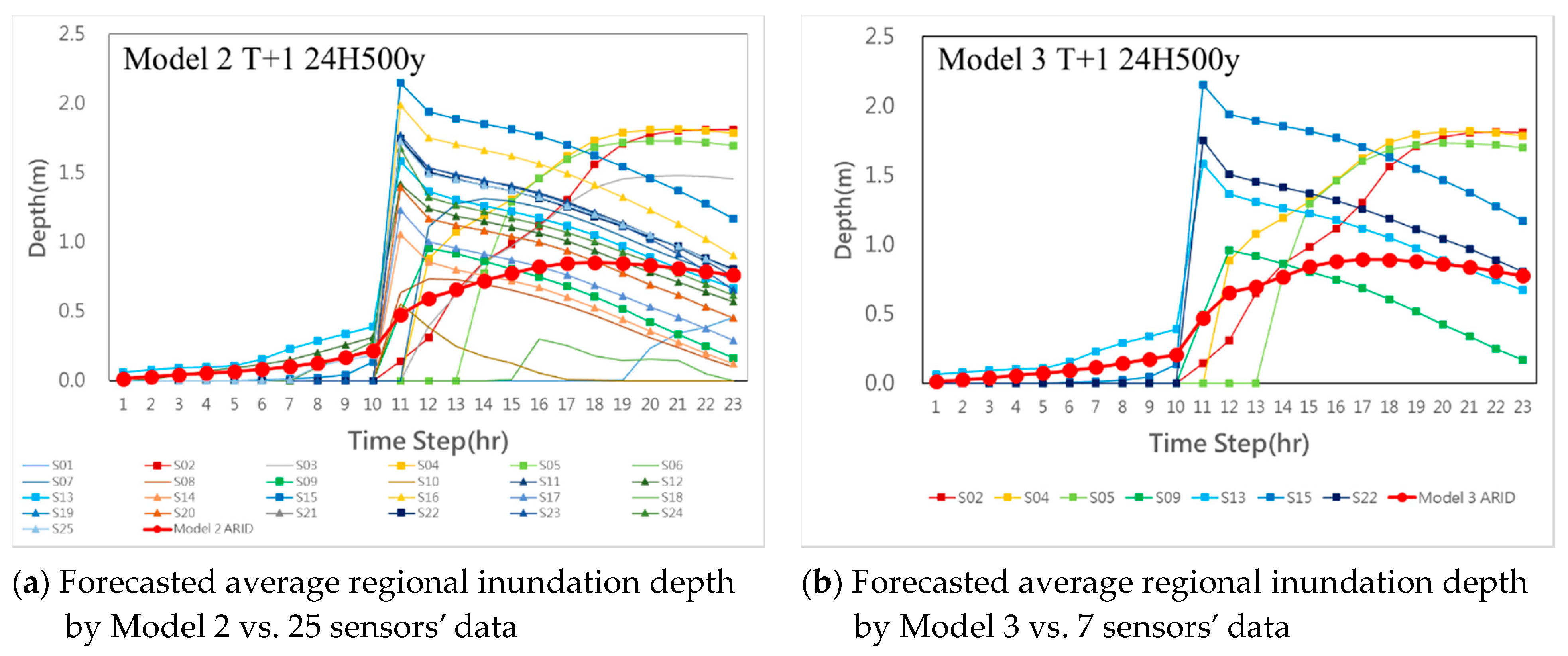
The hydrographs show 25 flood sensors and their correspondent ARID during the 500 year event used in Model 2 (Figure 6a) and 7 representative sensors used in Model 3 (Figure 6b), representatively. We noticed that many of these 25 sensors showed the same trend (such as $S_{11},S_{12},S_{13},S_{14},S_{15},S_{16},S_{17},S_{19},S_{20},S_{21},S_{23},S_{24},S_{25},$ etc.), which will result in additional parameters in the model and cause noise. In Model 3, which used only 7 representative sensors, the number of parameters and noise were both greatly reduced. Thus, the model could more accurately describe the relationship between rainfall, flooding sensor, and model output.

The evaluation indicators used in this study were RMSE (root-mean-square error), R², and Nash–Sutcliffe coefficient (NSE). The formulae are shown in Equations (15)–(17).

$$RMSE=\sqrt{\frac{{{\displaystyle \sum }}_{i=1}^N{\left(d_i-y_i\right)}^2}{N}}$$

(15)

$$R^2={\left(\frac{{{\displaystyle \sum }}_{i=1}^N\left(d_i-\overline{d}\right)\times \left(y_i-\overline{y}\right)}{\sqrt{{{\displaystyle \sum }}_{i=1}^N{\left(d_i-\overline{d}\right)}^2\times {{\displaystyle \sum }}_{i=1}^N{\left(y_i-\overline{y}\right)}^2}}\right)}^2$$

(16)

$$NSE=1-\frac{{{\displaystyle \sum }}_{i=1}^N{\left(d_i-y_i\right)}^2}{{{\displaystyle \sum }}_{i=1}^N{\left(d_i-\overline{d}\right)}^2}$$

(17)

where $d_i$ and $y_i$ are the observed value and the forecasted value of the ith data, respectively; $\overline{d}$ and $\overline{\mathrm{y}}$ are the means of the observed and forecasted values.

5. Results

As known, there is a temporal relationship between observations of the rainfall and IoT sensors’ inundation level of the study area and hence the value of observation at a particular time depends to some extent on past values. This study sought to model the temporal relationship and forecast the average regional inundation depth by using the machine learning model. Our reason for employing IoT sensor data was that the sensors could provide monitored (real) inundation values for model’s training as well as testing and thus improve the multi-step forecast accuracy. Moreover, the real-time monitoring datasets could be used to on-line adjust the model’s parameters and visually assess the model’s performance, which could largely promote the model’s applicability and reliability. The results of the three models are shown in

Table 3. Performance of one- to three-hour-ahead forecasts of the Model 1, Model 2, and Model 3.

Model		RMSE (m)			R2			NSE
	Time Step	Train	Val	Test	Train	Val	Test	Train	Val	Test
Model 1	T + 1	0.049	0.050	0.061	0.940	0.920	0.860	0.943	0.867	0.858
	T + 2	0.063	0.057	0.073	0.910	0.930	0.900	0.917	0.805	0.792
	T + 3	0.083	0.068	0.092	0.860	0.870	0.830	0.859	0.723	0.710
Model 2	T + 1	0.025	0.032	0.059	0.991	0.953	0.873	0.986	0.939	0.864
	T + 2	0.036	0.044	0.090	0.981	0.899	0.696	0.971	0.887	0.685
	T + 3	0.049	0.056	0.113	0.965	0.828	0.539	0.947	0.822	0.510
Model 3	T + 1	0.027	0.030	0.036	0.986	0.968	0.967	0.984	0.947	0.951
	T + 2	0.041	0.031	0.048	0.964	0.954	0.931	0.963	0.946	0.913
	T + 3	0.052	0.038	0.065	0.941	0.922	0.900	0.939	0.916	0.839

RMSE: root-mean-square error, NSE: Nash–Sutcliffe coefficient.

. There were two very large flood events (water depth > 0.5 m) in the training case. Model 1 results indicated those high flood events were underestimated, but its performances, in general, was good, where the RMSE could reach 0.049, 0.050, and 0.061 m in training, validation and testing cases, respectively. The small values of RMSE and high R² and NSE values indicate that Model 1, which was solely based on rainfall information as input, could provide suitable 1–3 h ahead forecasts, while it would largely underestimate the peak flood inundation depth.

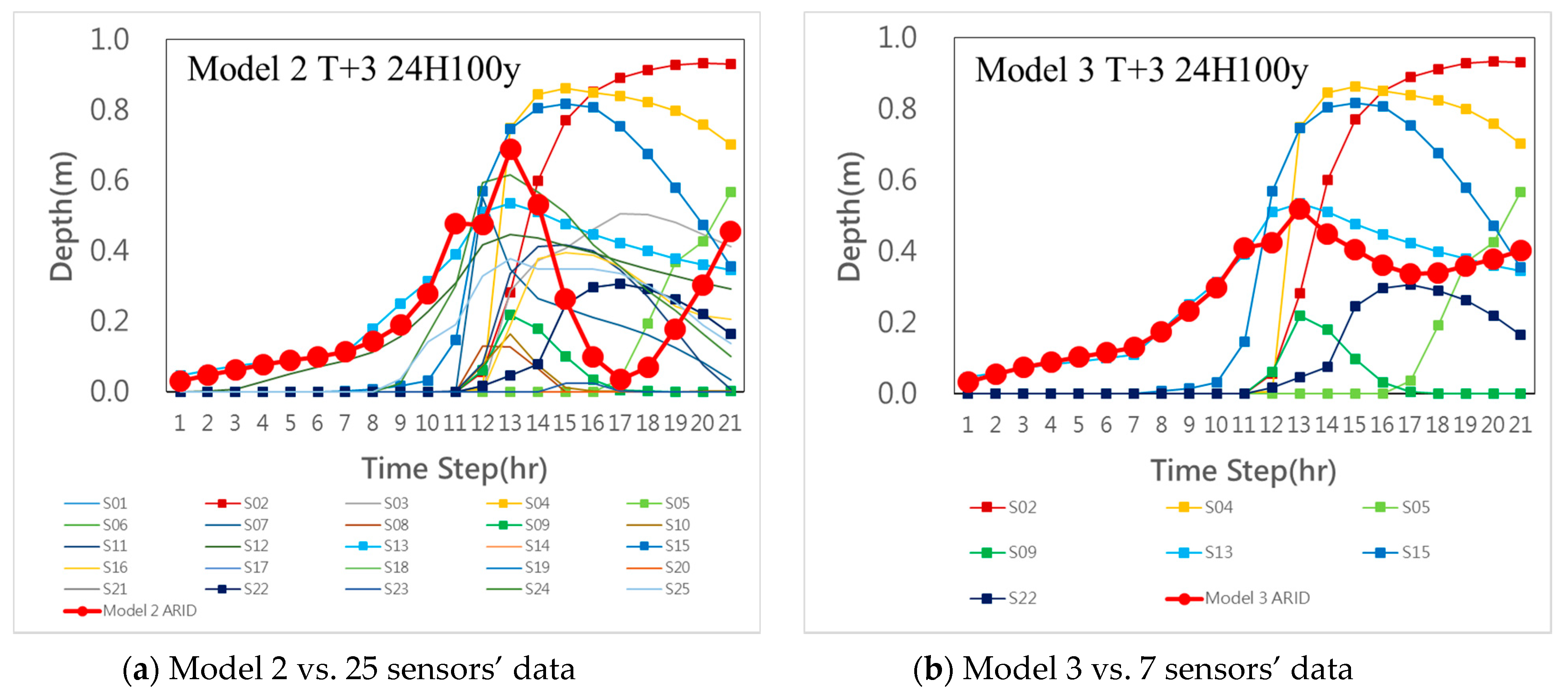
Model 2 used the data of 5 rainfall stations and 25 flood sensors. In the training phase, its errors in T + 1–T + 3 were significantly reduced as compared with those of Model 1. For instance, the RMSE values of Model 1 and Model 2 at T + 3 were 0.083 and 0.049, respectively. We notice that Model 2 had much better performances in multi-step-ahead forecasts (T + 1–T + 3) than those of Model 1 in the training phase, while that was not the case in both the validation and testing phases. In order to investigate the inconsistency problem, we explored the relationship between sensors’ data with the models’ forecast values in the event (24H100y) of the testing case. Figure 7a shows that the time series of 25 sensors were inconsistent, especially during the 12th–18th hours, where some of them were ascending, while the rest of them were descending, and the time series of the 3 h ahead forecasted ARID made by Model 2 was in sharp descent. We noticed that the inconsistency between sensors’ hydrographs might have been due to the propagation time between the upstream and downstream locations of the sensors resulting in the different lag time between the increasing and decreasing limb of their associated hydrograph. The inconsistency between the sensors’ datasets as well as the forecasted ARID values, however, could result in a large error (i.e., RMSE = 0.113 shown in Table 3). The results indicated that adding the IoT sensors information could, in general, reduce the forecast error of the ARID in the training phase due to using more information (25 sensors’ data) as input. Nevertheless, using a large number of inconsistent sensors values along the time series as input might introduce too many parameters in the model and result in an overfitting (overtraining) problem.

To reduce the input variables (sensors), correlation analysis was used to select a limited number of sensors as the representative sensors. Model 3 used the data of 5 rainfall stations and 7 representative sensors as inputs. Figure 7b shows the time series of 3 h forecasted ARID with the inundation depths of 7 representative sensors. As shown, the time series of 7 selected sensors as well as the forecasted ARID were relatively consistent, as compared with those of Figure 7a. The results show that Model 3, in general, was superior to the Model 1 and Model 2 in all the validation and testing phases, and its R² values in T + 1–T + 3 were consistent and higher than 0.9 in all the phases (Table 3). Thus, the Model 3 forecasts maintained fairly high accuracy (very small RMSE and high R² and NSE).

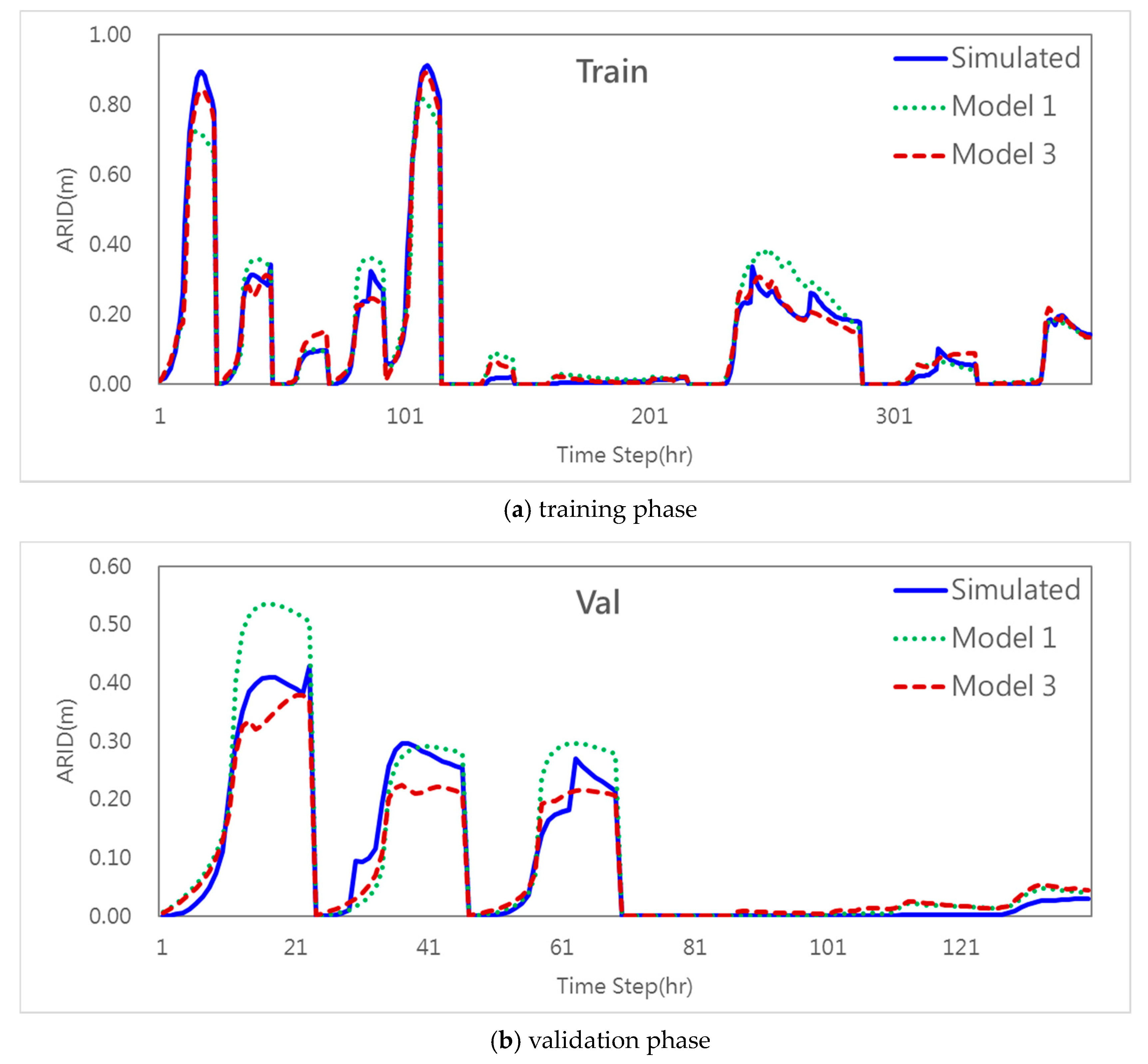
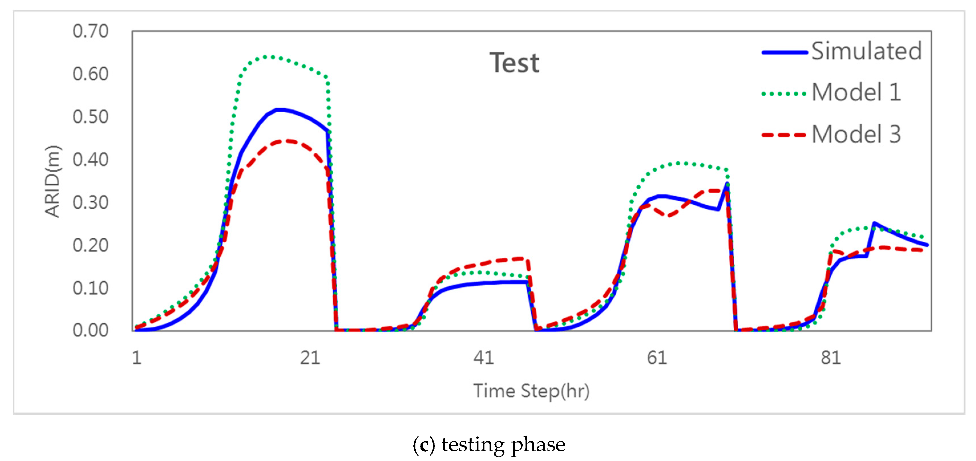
Figure 8 presents the forecast results of Model 1 and Model 3 at T + 1 in three phases. It shows that Model 1 underestimated the peak flow in the first and fifth events of the training session (i.e., 24H800mm and 24H500y), while they overestimated the peak flow in the validation and testing phases. In contrast, the results of Model 3 indicated that the problems of overestimated or underestimated peak values of ARIDs were significantly mitigated, its estimating errors (RMSE), in general, were also much smaller than those of Model 1 in all three phases.

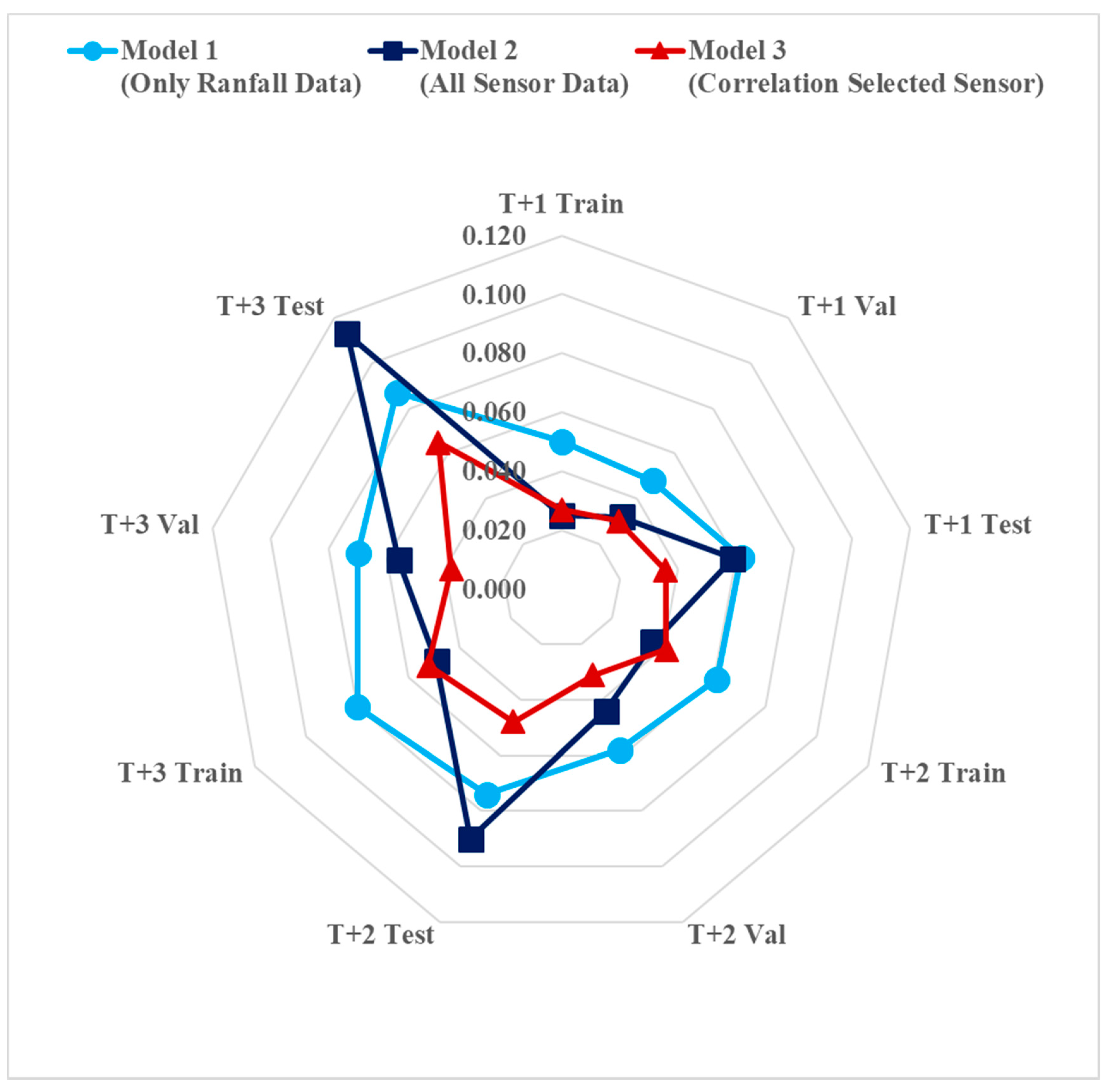
Figure 9 shows the RMSE charts in the training, validation, and testing phases of the three models. It is clearly shown that Model 3 had the most reliable and accurate performance compared to Models 1 and 2. Model 2 could be very well trained and was superior to Model 1 in all cases except in the cases of T + 2 and T + 3 in the testing phase, which was mainly caused by an inconsistency issue in the event of 24H100y. Model 3 had better performance than Model 2 in the validation and testing phases, where the average improvement rates were 22.65% and 42.71%, respectively. Moreover, the model’s weights were reduced from 166 (Model 2) to 76 (Model 3), when the number of parameters was significantly reduced by 54.21%. The analyzed results provide an extra evidence and demonstrate that using the selected sensors as model input not only produces a parsimonious model but also improves prediction accuracy in multi-step-ahead flood inundation forecasts. These results represent the great value and benefit of IoT sensors, which fuse as inputs into the machine learning models.

6. Conclusions

This study sought to model the temporal relationship and forecast the average regional inundation depth by using the IoT-based machine learning model. The datasets obtained from rainfall stations and IoT flood sensor data were used to model the average regional flood forecasts and explore the effectiveness and usefulness of the IoT sensors data in the model’s reliability and accuracy. The results show that adding IoT sensor data as a model input can reduce the model error, especially for those of long horizontal (T + 2 and T + 3) forecasts in high-flood-depth conditions, where their underestimations are significantly mitigated. For instance, by adding 25 IoT sensors of inundation depth as extra inputs of Model 2, an average error improvement rate up to 18.49% could be reached as compared with Model 1 (only used rainfall datasets). While we also noticed that the inconsistent relationship between the 25 sensors datasets could over train the model and result in a chaotic issue in late application. For instance, Model 2 does provide the worst performances in the testing phase of T + 3 case. On the other hand, Model 3 used 7 IoT representative sensors, selected by the principle of correlation, as the extra inputs to model the multi-step flood forecasts. The number of parameters of Model 3 were greatly reduced (over 50%) as compared with Model 2. Furthermore, Model 3 was superior to Model 2, with an average improvement rate up to 18%, and it also provided much better forecast performances (small RMSE and high R² and NSE values) than Model 1 in all the T + 1–T + 3 cases. Therefore, these results give very promising evidence and demonstrate that using the IoT representative sensors as the model input to configure the machine learning models not only can produce a parsimonious model but also significantly improve the models’ reliability and accuracy in multi-step-ahead regional flood inundation forecasts. The most fascinating achievement of this study is that the constructed model now can be on-line adjusted and its real-time forecast can be visually assessed and numerically evaluated based on the current implemented IoT inundation levels in the studied areas. Thus, the IoT-based machine learning model performance could be continuously assessed and adjusted, and its reliability and accuracy could be consistent.

References

- Kalyanapu, A.J.; Shankar, S.; Pardyjak, E.R.; Judi, D.R.; Burian, S.J. Assessment of GPU computational enhancement to a 2D flood model. Environ. Model. Softw. 2011, 26, 1009–1016. [Google Scholar] [CrossRef]
- Nayak, P.C.; Sudheer, K.P.; Rangan, D.M.; Ramasastri, K.S. Short-term flood forecasting with a neurofuzzy model. Water Resour. Res. 2005, 41. [Google Scholar] [CrossRef] [Green Version]
- Mai, D.T.; De Smedt, F. A combined hydrological and hydraulic model for flood prediction in Vietnam applied to the Huong river basin as a test case study. Water 2017, 9, 879. [Google Scholar] [CrossRef] [Green Version]
- Adamowski, J.; Chan, H.F.; Prasher, S.O.; Ozga-Zielinski, B.; Sliusarieva, A. Comparison of multiple linear and nonlinear regression, autoregressive integrated moving average, artificial neural network, and wavelet artificial neural network methods for urban water demand forecasting in Montreal, Canada. Water Resour. Res. 2012, 48. [Google Scholar] [CrossRef]
- Rezaeianzadeh, M.; Tabari, H.; Yazdi, A.A.; Isik, S.; Kalin, L. Flood flow forecasting using ANN, ANFIS and regression models. Neural Comput. Appl. 2014, 25, 25–37. [Google Scholar] [CrossRef]
- Zare, M.; Koch, M. An analysis of MLR and NLP for use in river flood routing and comparison with the Muskingum method. In Proceedings of the ICHE 2014—11th International Conference on Hydroscience & Engineering, Hamburg, Germany, 28 September–2 October 2014; pp. 505–514. Available online: https://henry.baw.de/bitstream/handle/20.500.11970/99469/06_16.pdf?sequence=1&isAllowed=y (accessed on 31 May 2020).
- Valipour, M.; Banihabib, M.E.; Behbahani, S.M.R. Comparison of the ARMA, ARIMA, and the autoregressive artificial neural network models in forecasting the monthly inflow of Dez dam reservoir. J. Hydrol. 2013, 476, 433–441. [Google Scholar] [CrossRef]
- Huang, Y.F.; Mirzaei, M.; Yap, W.K. Flood analysis in Langat river basin using stochastic model. Int. J. Geomate. 2016, 11, 2796–2803. [Google Scholar]
- Ab Razak, N.H.; Aris, A.Z.; Ramli, M.F.; Looi, L.J.; Juahir, H. Temporal flood incidence forecasting for Segamat River (Malaysia) using autoregressive integrated moving average modelling. J. Flood Risk Manag. 2018, 11, S794–S804. [Google Scholar] [CrossRef]
- Machekposhti, K.H.; Sedghi, H.; Telvari, A.; Babazadeh, H. Flood Predicting in Karkheh River Basin Using Stochastic ARIMA Model. Int. J. Agric. Biosyst. Eng. 2018, 12, 89–96. [Google Scholar]
- Kan, G.; He, X.; Ding, L.; Li, J.; Liang, K.; Hong, Y. Study on applicability of conceptual hydrological models for flood forecasting in humid, semi-humid semi-arid and arid basins in China. Water 2017, 9, 719. [Google Scholar] [CrossRef] [Green Version]
- Chiang, Y.M.; Chang, L.C.; Tsai, M.J.; Wang, Y.F.; Chang, F.J. Dynamic neural networks for real-time water level predictions of Sewerage systems-covering gauged and unguaged sites. Hydrol. Earth Syst. Sci. 2010, 14, 1309–1319. [Google Scholar] [CrossRef] [Green Version]
- Chang, F.J.; Chen, P.A.; Liu, C.W.; Liao, V.H.C.; Liao, C.M. Regional estimation of groundwater arsenic concentrations through systematical dynamic-neural modeling. J. Hydrol. 2013, 499, 265–274. [Google Scholar] [CrossRef]
- Ruslan, F.A.; Samad, A.M.; Zain, Z.M.; Adnan, R. Flood water level modeling and prediction using NARX neural network: Case study at Kelang river. In Proceedings of the 2014 IEEE 10th International Colloquium on Signal Processing and its Applications IEEE, Kuala Lumpur, Malaysia, 7–9 March 2014; pp. 204–207. [Google Scholar] [CrossRef]
- Mosavi, A.; Ozturk, P.; Chau, K.W. Flood prediction using machine learning models: Literature review. Water 2018, 10, 1536. [Google Scholar] [CrossRef] [Green Version]
- Noymanee, J.; Nikitin, N.O.; Kalyuzhnaya, A.V. Urban pluvial flood forecasting using open data with machine learning techniques in pattani basin. Procedia Comput. Sci. 2017, 119, 288–297. [Google Scholar] [CrossRef]
- Puttinaovarat, S.; Horkaew, P. Flood Forecasting System Based on Integrated Big and Crowdsource Data by Using Machine Learning Techniques. IEEE Access 2020, 8, 5885–5905. [Google Scholar] [CrossRef]
- PB, L.P.; Bhakthavathsalam, R.; Vishruth, K. Urban Flood Forecast using Machine Learning on Real Time Sensor Data. Trans. Mach. Learn. Artif. Intell. 2017, 5, 69. Available online: https://journals.scholarpublishing.org/index.php/TMLAI/article/view/3552/2104 (accessed on 31 May 2020). [CrossRef]
- Tayfur, G.; Singh, V.P.; Moramarco, T.; Barbetta, S. Flood hydrograph prediction using machine learning methods. Water 2018, 10, 968. [Google Scholar] [CrossRef] [Green Version]
- Leontaritis, I.J.; Billings, S.A. Input-output parametric models for non-linear systems Part I: Deterministic non-linear systems, Part II: Stochastic non-linear systems. Int. J. Control 1985, 41, 303–344. [Google Scholar] [CrossRef]
- Tian, C.; Horne, R.N. Recurrent neural networks for permanent downhole gauge data analysis. In SPE Annual Technical Conference and Exhibition; Society of Petroleum Engineers: Calgary, AB, Canada, 2017. [Google Scholar] [CrossRef]
- Koschwitz, D.; Frisch, J.; Van Treeck, C. Data-driven heating and cooling load predictions for non-residential buildings based on support vector machine regression and NARX Recurrent Neural Network: A comparative study on district scale. Energy 2018, 165, 134–142. [Google Scholar] [CrossRef]
- Abou Rjeily, Y.; Abbas, O.; Sadek, M.; Shahrour, I.; Hage Chehade, F. Flood forecasting within urban drainage systems using NARX neural network. Water Sci. Technol. 2017, 76, 2401–2412. [Google Scholar] [CrossRef]
- Khalid, E.G.; Jamal, E.K.; Isam, S.; Aziz, S. Comparison of M5 Model Tree and Nonlinear Autoregressive with eXogenous inputs (NARX) Neural Network for urban stormwater discharge modelling. In MATEC Web of Conferences; EDP Sciences: Les Ulis, France, 2019; Volume 295, p. 02002. [Google Scholar] [CrossRef]
- Zainorzuli, S.M.; Abdullah, S.A.C.; Adnan, R.; Ruslan, F.A. Comparative Study of Elman Neural Network (ENN) and Neural Network Autoregressive with Exogenous Input (NARX) For Flood Forecasting. In Proceedings of the 2019 IEEE 9th Symposium on Computer Applications & Industrial Electronics (ISCAIE), Kota Kinabalu, Sabah, Malaysia, 27–28 April 2019; IEEE: Piscataway, NJ, USA, 2019; pp. 11–15. [Google Scholar] [CrossRef]
- Chang, F.J.; Chen, P.A.; Lu, Y.R.; Huang, E.; Chang, K.Y. Real-time multi-step-ahead water level forecasting by recurrent neural networks for urban flood control. J. Hydrol. 2014, 517, 836–846. [Google Scholar] [CrossRef]
- Shen, H.Y.; Chang, L.C. Online multistep-ahead inundation depth forecasts by recurrent NARX networks. Hydrol. Earth Syst. Sci. 2013, 17, 935–945. [Google Scholar] [CrossRef] [Green Version]
- Chang, L.C.; Shen, H.Y.; Chang, F.J. Regional flood inundation nowcast using hybrid SOM and dynamic neural networks. J. Hydrol. 2014, 519, 476–489. [Google Scholar] [CrossRef]
- Chang, L.C.; Amin, M.Z.M.; Yang, S.N.; Chang, F.J. Building ANN-based regional multi-step-ahead flood inundation forecast models. Water 2018, 10, 1283. [Google Scholar] [CrossRef] [Green Version]
- Bande, S.; Shete, V.V. Smart flood disaster prediction system using IoT & neural networks. In Proceedings of the 2017 International Conference On Smart Technologies For Smart Nation (SmartTechCon), Bengaluru, India, 17–19 August 2017; IEEE: Piscataway, NJ, USA; pp. 189–194. [Google Scholar] [CrossRef]
- Babu, V.; Rajan, V. Flood and Earthquake Detection and Rescue Using IoT Technology. In Proceedings of the 2019 International Conference on Communication and Electronics Systems (ICCES), Coimbatore, India, 17–19 July 2019; IEEE: Piscataway, NJ, USA; pp. 1256–1260. [Google Scholar] [CrossRef]
- Wang, Y.; Chen, X.; Wang, L.; Min, G. Effective IoT-Facilitated Storm Surge Flood Modeling Based on Deep Reinforcement Learning. In IEEE Internet of Things Journal; IEEE: Piscataway, NJ, USA, 2020. [Google Scholar] [CrossRef]
- Han, K.; Zhang, D.; Bo, J.; Zhang, Z. Hydrological monitoring system design and implementation based on IOT. Phys. Procedia 2012, 33, 449–454. [Google Scholar] [CrossRef] [Green Version]
- Wang, J.; Yang, X. An Automatic Online Disaster Monitoring Network: Network Architecture and a Case Study Monitoring Slope Stability. Int. J. Online Biomed. Eng. 2018, 14, 4–19. [Google Scholar] [CrossRef]
- Puttinaovarat, S.; Horkaew, P. Application Programming Interface for Flood Forecasting from Geospatial Big Data and Crowdsourcing Data. Int. J. Interact. Mob. Technol. 2019, 13, 137–156. [Google Scholar] [CrossRef]
- Basha, E.A.; Ravela, S.; Rus, D. Model-based monitoring for early warning flood detection. In SenSys ’08: Proceedings of the 6th ACM Conference on Embedded Network Sensor Systems; ACM: New York, NY, USA, 2008; pp. 295–308. [Google Scholar] [CrossRef] [Green Version]
- Mitra, P.; Ray, R.; Chatterjee, R.; Basu, R.; Saha, P.; Raha, S.; Barman, R.; Patra, S.; Biswas, S.S.; Saha, S. Flood forecasting using Internet of things and artificial neural networks. In Proceedings of the 2016 IEEE 7th Annual Information Technology, Electronics and Mobile Communication Conference (IEMCON), Vancouver, BC, Canada, 13–15 October 2016; IEEE: Piscataway, NJ, USA; pp. 1–5. [Google Scholar] [CrossRef]
- Pasi, A.A.; Bhave, U. Flood detection system using wireless sensor network. Int. J. Adv. Res. Comput. Sci. Softw. Eng. 2015, 5. [Google Scholar] [CrossRef]
- Chang, L.C.; Chang, F.J.; Yang, S.N.; Kao, I.F.; Ku, Y.Y.; Kuo, C.L.; bin Mat, M.Z. Building an intelligent hydroinformatics integration platform for regional flood inundation warning systems. Water 2019, 11, 9. [Google Scholar] [CrossRef] [Green Version]
- Sood, S.K.; Sandhu, R.; Singla, K.; Chang, V. IoT, big data and HPC based smart flood management framework. Sustain. Comput. Inform. Syst. 2018, 20, 102–117. [Google Scholar] [CrossRef] [Green Version]
- Mishra, B.K.; Thakker, D.; Mazumdar, S.; Neagu, D.; Simpson, S. Using Deep Learning for IoT-enabled Smart Camera: A Use Case of Flood Monitoring. In Proceedings of the 2019 10th International Conference on Dependable Systems, Services and Technologies (DESSERT), Leeds, UK, 5–7 June 2019. [Google Scholar] [CrossRef]
- Bowden, G.J.; Dandy, G.C.; Maier, H.R. Input determination for neural network models in water resources applications. Part 1—background and methodology. J. Hydrol. 2005, 301, 75–92. [Google Scholar] [CrossRef]
- Galelli, S.; Humphrey, G.B.; Maier, H.R.; Castelletti, A.; Dandy, G.C.; Gibbs, M.S. An evaluation framework for input variable selection algorithms for environmental data-driven models. Environ. Model. Softw. 2014, 62, 33–51. [Google Scholar] [CrossRef] [Green Version]
- Hu, J.H.; Tsai, W.P.; Cheng, S.T.; Chang, F.J. Explore the relationship between fish community and environmental factors by machine learning techniques. Environ. Res. 2020, 184, 109262. [Google Scholar] [CrossRef] [PubMed]
- Muttil, N.; Chau, K.W. Machine-learning paradigms for selecting ecologically significant input variables. Eng. Appl. Artif. Intell. 2007, 20, 735–744. [Google Scholar] [CrossRef] [Green Version]
- Taormina, R.; Chau, K.W. Data-driven input variable selection for rainfall–runoff modeling using binary-coded particle swarm optimization and extreme learning machines. J. Hydrol. 2015, 529, 1617–1632. [Google Scholar] [CrossRef]
- Chang, F.J.; Chen, P.A.; Chang, L.C.; Tsai, Y.H. Estimating spatio-temporal dynamics of stream total phosphate concentration by soft computing techniques. Sci. Total Environ. 2016, 562, 228–236. [Google Scholar] [CrossRef]
Figure 1.
The architecture of the recurrent nonlinear autoregressive with exogenous inputs (RNARX) network.
Figure 2.
Study area of Erren river catchment.
Figure 3.
Rainfall histogram and average regional inundation depth hydrograph for training events. (a) 24H800 mm; (b) 24H450 mm; (c) 24H200 mm; (d) 24H10 y; (e) 24H500 y; (f) 20190719; (g) 20170601; (h) 20160925; (i) 20160912; (j) 20190813.
Figure 4.
Research framework.
Figure 5.
The procedure of selecting representative sensors.
Figure 6.
The sensor data vs. T + 1 forecasted average regional inundation depths by Models. (a) 25 sensors’ data vs. T+1 forecasted ARIDs of Model 2; (b) 7 sensors’ data vs. T+1 forecasted ARIDs of Model 3.
Figure 7.
The sensor data vs. T + 3 forecasted average regional inundation depths by Models. (a) 25 sensors’ data vs. T+3 forecasted ARIDs of Model 2; (b) 7 sensors’ data vs. T+3 forecasted ARIDs of Model 3.
Figure 8.
Comparison of simulation, Model 1, and Model 3 in three phases. (a) training phase; (b)validation phase; (c)testing phase.
Figure 9.
The radar chart of models’ performance (RMSE) in three phases.