A New Formulation for the Capacitated Lot Sizing Problem with Batch Ordering Allowing Shortages

Abstract

This paper addresses the multi-product, multi-period capacitated lot sizing problem. In particular, this work determines the optimal lot size allowing for shortages (imposed by budget restrictions), but with a penalty cost. The developed models are well suited to the usually rather inflexible production resources found in retail industries. Two models are proposed based on mixed-integer formulations: (i) one that allows shortage and (ii) one that forces fulfilling the demand. Both models are implemented over test instances and a case study of a real industry. By investigating the properties of the obtained solutions, we can determine whether the shortage allowance will benefit the company. The experimental results indicate that, for the test instances, the fact of allowing shortages produces savings up to 17% in comparison with the model without shortages, whereas concerning the current situation of the company, these savings represent 33% of the total costs while preserving the revenue.

1. Introduction

Today’s companies are immersed in a globalized market crammed with considerable demands for different products. Regardless of the size or type of industry, the selling business always involves two parties: customers and sellers. Customers search for quality products that meet their requirements, whereas companies search for adaptive strategies to compete against each other and satisfy the preferences of their individual customers while minimizing any negative impact on their operations and other aspects of their businesses [1].

One of the most integral operations of a company is inventory management, because many resources are expended on goods and products that will generate profits for the company. Yet, the purchased materials must be ordered at an economic price and then stored. On the other hand, companies that sell products in large quantities or with high variability in their demand commonly face the overstock problem, wherein the optimum stocking level is exceeded, and the stored products cannot be sold beyond an estimated time. This is the problem faced by a Mexican textile and footwear distributor that inspired this research. This company handles several products in catalogues and sells them to wholesale and retail customers. Currently, the company manually gathers the data that allow the analysts and sales force to understand the products’ behaviours and, consequently, plan the most appropriate purchase strategy. This data collection process is merely supported by the empirical sui generis methods of older, more experienced workers. Coupled with this problem, suppliers place product-dependent batch orders of different sizes with the company. The delivery time of each item is established by the corresponding supplier and hinders the empirical purchasing planning conducted by the company. Thus, the present work develops a couple of Mixed-Integer Linear Programming (MILP) models for inventory management. The two MILP models involve multiple items and multiple periods, including different capacity constraints related to the batch size, lead time, and budget. These models seek to improve the timing and quantity of the ordering scheme, thereby reducing the operating expenses of the company. The effectiveness of these formulations is evaluated through the case study. The remaining sections of this paper are organized as follows. Section 2 reviews the relevant literature, and Section 3 introduces the proposed MILP formulations. In Section 4, the proposed models are implemented and evaluated in the case study of a Mexican fashion retail company. Section 5 presents the conclusions and some directions for future research.

2. Literature Review

Interest in streamlining inventory processes has recently increased, particularly in tasks related to classifying products, registration methods, and re-inventory models. According to De Horatius [2], inventory management focuses on minimizing the inventory levels while ensuring stock availability. Inventory planning then is a fundamental part of the fashion retail industry, which covers the business of fashion products such as apparel, shoes, and beauty products. This fashion market is very challenging as it is characterized by short life cycles compared to other retail and service industries, high volatility, poor predictability, and critical-mass shopping behaviour [1]. As Liu et al. [3] stated, retailers’ optimal management of their inventories largely depends on the accuracy of predicting future demand, which is commonly affected by uncertainty factors that are difficult to manage, such as trends, seasonality, and availability.

The history of inventory problems is rooted in the Economic Order Quantity (EOQ) model, which assumes a single item in a continuous and constant demand over an infinite planning horizon. This EOQ model is easily solved to determine the optimal order quantity, balancing the setups, and computing the inventory holding costs. However, the model becomes NP-hard when more items are considered and multiple capacity restrictions are in place [4]. Thus, this problem has been extended to considering multiple items under the imposition of different cost conditions and limited production capacities, which in turn have culminated in the known Capacitated Lot Sizing Problem (CLSP). Furthermore, the combination of these considerations, along with additional features such as the demand uncertainty, setup costs and/or time, and alternative suppliers have introduced different complexities to address the problem [5]. Hence, every firm must decide the lot sizing problem with the specific considerations that are better suited to describe its current circumstances and that will directly affect its system operation, productivity, and overall performance.

The general CLSP problem seeks to optimize the order quantity that will meet the customer demand, over a finite time horizon, while minimizing the sum of ordering, purchasing, and holding inventory costs. Although constraints in the formulation of this problem might limit the production, space, or budget capacity for any given product, the basic mathematical model is easily adapted by appropriately interpreting the model elements, such as the variables and parameters [5].

The lot sizing problem has been studied since the early Twentieth Century, and its application in real scenarios currently constitute an active area of research [6,7,8]. Moreover, this problem has split into a wide diversity of variants to the problem, which in turn have been solved by an even wider variety of approaches. In this regard, different reviews summarizing the literature available have been published since the mid 1990s [9,10,11,12,13,14,15,16]. Overall, this literature can be classified into three groups: (1) studies considering space or monetary budgets; (2) studies on lead time; and (3) studies considering batch size.

First, among the studies considering space or monetary budgets, Ben-Daya and Raouf [17] developed an algorithm that optimizes the ordering policy in the multi-item, single-period inventory problem, within the context of perishable commodities. In this study, the algorithm determines the setup costs and lot size decisions when items compete for budgetary and floor- or shelf-space restrictions. Any shortage is translated into a penalty cost, and the excess of products (above demand) is disposed at a reduced price. Nonetheless, the policy is fixed during the planning horizon and does not consider the possibility of replenishment. A few years later, Guan and Li [18] presented two models of lot size, one with a restricted storage capacity and a second with a constraint on the order capacity. Meanwhile, a different study was developed by Fan and Wang [19], who modelled a lot size problem that sought to reduce ordering and storing expenses in a scenario where the size of the warehouse could be altered at a cost for each change in capacity. One more study was conducted by Woarawichai et al. [20], who developed an MILP for the multi-period inventory lot size problem with supplier selection under storage and budget constraints. The authors introduced a supplier-dependent transaction cost, but the order lead time was deterministic and assumed identical for all products, which limited the contribution of the model.

Second, among the studies on lead time, Karmarkar [21] related the lead time to lot size and concluded that extending the lead time negatively affected the response to customers. The author also argued that small batches created more setups while large batches lengthened the lead time. Some years later, Ben-Daya and Raouf [22] reviewed different inventory models that considered the lead time and order quantity as decision variables. However, most of the revised works assumed an invariant lead time over the entire planning horizon. For this reason, Kuik et al. [9] defined these models as finite capacity models. Meanwhile, Hariga and Ben-Daya [23] developed a continuous-review inventory model in which the reorder point, the ordering quantity, and the lead time were the decision variables, followed by Ouyang, Chen, and Chang [24], who studied a reorder-point inventory model with a variable lead time and partial backorders in an imperfect production process. These authors similarly defined the lead time as a decision variable to be minimized, in combination with other variables such as lot size, reorder point, process quality, and setup cost. A more recent study conducted by Helber and Sahling [25] solved a dynamic multilevel CLSP with positive lead times by a mathematical programming approach. Here, the authors developed an iterative procedure that fixed the products to be purchased in each period and then optimized the lot size of each purchased item. They developed four variants of this procedure with different decomposition structures to diversify the search in the solution space.

Finally, among studies considering batch size, more recent studies have been carried out. For example, Yang et al. [26] analyzed the optimal inventory management of a single product that is purchased in batches. This method accounts for the placement cost in a limited warehouse capacity. A different algorithm was later proposed by Akbalik et al. [27], who addressed a company that buys its products in batches and varies the storage cost when supply exceeds the determined capacity. At the same time, Farhat et al. [28] studied batch purchases with the option of returning the items that were not sold to the supplier. When the products purchased in batches are perishable, they must be treated with special care, and the model must consider a series of constraints, as proposed by Broekmeulen and van Donselaar [29].

As shown in this section, there is a vast literature addressing different variants of the lot sizing problem. Yet, literature focusing on optimizing the CLSP by considering variable batch sizes and variable delivery times (lead times) in retail applications is very scarce. In addition, many articles apply discounts when buying in large volumes, which is managed differently by the company under study.

3. Problem Statement

The problem analyzes a retailer who buys products in large quantities (lot sizes) from manufacturers and then sells them in smaller quantities (possibly single units) to consumers. The ordered quantities are merely considered as integer multiples of the batch size of each item. The retailer, should decide “what products to order”, “how much to order for each product”, and “when to order”.

Unlike common lot sizing models in manufacturing environments, in our model, the retailers depend mainly on the lead time ($LT$) established by the suppliers. To ensure their timely receipt, purchase orders must be placed ahead of time (i.e., in advance). This anticipation is represented by an artificial shift ($ST$) created over the planning horizon, where the periods to be phased out are added before the first week of demand.

The following example attempts to show how the artificial shift over the time horizon periods will work. The instance considers three products to be purchased within a planning horizon of six ($r=6$) periods ($1,\dots ,r$). Item 1 belongs to imported products, i.e., is provided by an external supplier. The demand for each product in each period is displayed in

Table 1. Demands per item and period for the original planning horizon.

	1	…				r
Item/Demand	1	2	3	4	5	6
1	110	99	164	181	95	164
2	197	120	146	101	152	131
3	174	132	137	142	119	183

.

The lead time ($LT$) of items 1, 2, and 3 are 3, 1, and 2 periods, respectively. The batch sizes of Items 1, 2, and 3 are 200, 200, and 150 units, respectively.

To create the shifted horizon ($ST$), we must determine the maximum number of periods that must be added to the horizon planning time. We assume that the maximum lead time ($LTmax$) is the maximum $LT$ of the imported products ($LTmax=3$ in this example). Therefore, the end of the time horizon is shifted from the sixth (r) to the ninth period ($s=r+L{T}_{max}$).

Table 2. Demand per item and per period for the shifted planing horizon.

	1	…				r	…		s
Item/Period	1	2	3	4	5	6	7	8	9
1	0	0	0	110	99	164	181	95	164
2	0	0	0	197	120	146	101	152	131
3	0	0	0	174	132	137	142	119	183

shows the corresponding demands over the $ST$ shifted horizon in the illustrative example.

As shown in Table 2, the first three periods represent the artificial shift (with zero demand values). From the fourth to the ninth period, the demands correspond to those of the original planning horizon (Table 1).

Since the company has the policy of paying the orders in advance (to seize the discount prices), we formulated the model to take into account this feature. For this reason, we considered the shifted time horizon, in which the company can place the orders $L{T}_i$ periods ahead (depending on the item) of the period in which they will be sold. To avoid dealing with negative indices, the first demand period is shifted to the $L{T}_{max}+1$ period.

3.1. Mathematical Formulation

In this section, we formally define the addressed problem and propose an MILP formulation. Prior to that, let us introduce the following sets and parameters:

$N:$	Set of n items to sell, indexed by i, where $i\in \{1,\dots ,n\}.$
$M:$	Set of m imported items, the first m items from N, $M\subset N$, indexed by j, where $j\in \{1,\dots ,m\}.$
$T:$	Set of r original time horizon periods, indexed by h, where $h\in \{1,\dots ,r\}.$
$ST:$	Set of s shifted periods, indexed by t, where $t\in \{L{T}_{max}+1,\dots ,s\}.$
$D_{it}:$	Demand for item i at period t.
$T{D}_i:$	Total demand per item i, expressed as the sum of the periodical demands over the time horizon.
$O_i:$	Setup order cost for item i.
$P_i:$	Unitary purchase cost for item i.
$H_i:$	Holding cost for item i.
$W_{ini}:$	Initial purchase budget.
$W_t:$	Periodical budget (after the initial purchase) for period t.
$L{T}_i:$	Lead time of item i.
$L{T}_{max}:$	Maximum lead time over imported items.
$B_i:$	Batch size of item i (in number of units).
$S_i:$	Penalty shortage cost for every unit of item i.

Two particular features must be considered in the proposed model. On the one hand, the company classifies the items into two categories: imported (purchased from external suppliers) and domestic (acquired from internal manufacturers). On the other hand, imported items share a common lead time that requires the placing of future orders. Therefore, for them, only an initial order must be placed. For this reason, imported items represent the first items in the N set.

3.2. MILP Formulation with Shortages

The problem consists of determining the purchase orders, i.e., the quantity of batches to be purchased per item over the planning period, in such a way that the total cost incurred by the holding, shortages, and final inventory costs are minimized. We also determined the maximum inventory levels in order to take advantage of the availability of space in the warehouse.

Let us introduce the following decision variables to establish the mathematical model:

$$\begin{array}{ccc}\hfill X_{it}& =& \mathrm{Quantity}\mathrm{of}\mathrm{batches}\mathrm{of}\mathrm{item}i\mathrm{to}\mathrm{purchase}\mathrm{at}\mathrm{period}t.\hfill \\ \hfill I_{it}& =& \mathrm{Quantity}\mathrm{of}\mathrm{units}\mathrm{of}\mathrm{item}i\mathrm{to}\mathrm{hold}\mathrm{in}\mathrm{inventory}\mathrm{at}\mathrm{period}t.\hfill \\ \hfill Z_{it}& =& \mathrm{Quantity}\mathrm{of}\mathrm{shortage}\mathrm{units}\mathrm{of}\mathrm{item}i\mathrm{at}\mathrm{period}t.\hfill \\ \hfill R_i& =& \mathrm{Maximum}\mathrm{allowed}\mathrm{inventory}\mathrm{of}\mathrm{item}i\mathrm{in}\mathrm{any}\mathrm{period}.\hfill \\ \hfill Y_{it}& =& \left\{\begin{array}{cc}1,\hfill & \mathrm{if}\mathrm{purchase}\mathrm{order}i\mathrm{is}\mathrm{placed}\mathrm{at}\mathrm{period}t\hfill \\ 0,\hfill & \mathrm{otherwise}.\hfill \end{array}\right.\hfill \end{array}$$

The objective function (1) aims to minimize three terms: the holding cost, the shortage cost, and the final inventory costs. The third term is considered only over the last period stock per item.

$$\mathrm{Minimize}\sum _{i=1}^n\sum _{t=1}^{s-1}{H}_i{I}_{it}+\sum _{i=1}^n\sum _{t=1}^s{S}_i{Z}_{it}+2\sum _{i=1}^n{P}_i{I}_{is}.$$

(1)

The balance equation for item i in period t (equals the sum of the inventory over the previous period and the purchase in the current period, minus the remaining surplus in the current period) is established by Equation (2).

$$\begin{array}{ccc}\hfill I_{i(t-1)}+B_i{X}_{i(t-L{T}_i)}-D_{it}+Z_{it}& =& I_{it},\forall i\in N;t\in ST.\hfill \end{array}$$

(2)

The maximum allowable inventory of each item in each period is ensured by Equation (3). Meanwhile, Equation (4) ensure that, for each item, no inventory is generated before the $L{T}_{max}$ period.

$$\begin{array}{ccc}\hfill I_{it}& \le & R_i,\forall i\in N,t\in ST,\hfill \end{array}$$

(3)

$$\begin{array}{ccc}\hfill I_{ih}& =& 0,\forall i\in N,h\in T,h\le L{T}_{max}.\hfill \end{array}$$

(4)

For imported items, only one purchase order must be placed, and it should be placed at the beginning of the time horizon; this is ensured by Equation (5).

$$\begin{array}{ccc}\hfill \sum _{\begin{array}{c}t=L{T}_{max}+2\end{array}}^s{Y}_{j(t-L{T}_i)}& =& 0,\forall j\in M.\hfill \end{array}$$

(5)

The amount of the initial purchase cannot exceed the budget assigned at the first original time period; this is ensured by Equation (6), while the total lot size based on the weekly budget is ensured by Equation (7).

$$\begin{array}{ccc}\hfill {\displaystyle \sum _{\begin{array}{c}i=1\end{array}}^n(B_i{P}_i{X}_{i(L{T}_{max}-L{T}_i+1)}+O_i{Y}_{i(L{T}_{max}-L{T}_i+1)})}& \le & W_{ini},\hfill \end{array}$$

(6)

$$\begin{array}{ccc}\hfill {\displaystyle \sum _{\begin{array}{c}i=m+1\end{array}}^n(B_i{P}_i{X}_{i(t-L{T}_i)}+O_i{Y}_{i(t-L{T}_i)})}& \le & W_t,\forall t\in ST,t>L{T}_{max}+1.\hfill \end{array}$$

(7)

Based on the batch size of each item, the maximum allowable quantity of purchased batches (in general) of item i is determined by Equation (8).

$$\begin{array}{ccc}\hfill X_{i(t-L{T}_i)}& \le & \left(1+\frac{T{D}_i}{B_i}\right)Y_{i(t-L{T}_i)},\forall i\in N;t\in ST.\hfill \end{array}$$

(8)

The units of shortage per item and per period is estimated by Equations (9) and (10), respectively.

$$\begin{array}{ccc}\hfill Z_{it}& \ge & D_{it}-B_i{X}_{it}-I_{it},\forall i\in N;t\in ST,\hfill \end{array}$$

(9)

$$\begin{array}{ccc}\hfill Z_{it}& \le & D_{it},\forall i\in N;t\in ST.\hfill \end{array}$$

(10)

The nature of the variables is established by the group of Equations (11)–(15).

$$\begin{array}{ccc}\hfill R_i& \ge & 0,\forall i\in N,\hfill \end{array}$$

(11)

$$\begin{array}{ccc}\hfill I_{it}& \ge & 0,\forall i\in N;t\in ST,\hfill \end{array}$$

(12)

$$\begin{array}{ccc}\hfill X_{it}& \ge & 0,\forall i\in N;t\in ST,\hfill \end{array}$$

(13)

$$\begin{array}{ccc}\hfill Z_{it}& \ge & 0,\forall i\in N;t\in ST,\hfill \end{array}$$

(14)

$$\begin{array}{ccc}\hfill Y_{it}& \in & \{0,1\},\forall i\in N;t\in ST.\hfill \end{array}$$

(15)

This model will be referred to as the “AS model” in the computational experiments section.

Let us continue with the illustrative example of Section 3. The optimal solution has an objective function value of $33,895.40.

Table 3. Optimal purchase orders during the shifted planning horizon.

Item/Period	1	2	3	4	5	6	7	8	9
1	4	0	0	0	0	0	0	0	0
2	0	1	1	1	0	1	0	0	0
3	0	0	2	1	0	1	1	1	0

shows the purchase orders of each item over the planning period.

During the first three periods, the purchases listed in Table 3 satisfy the demands in the fourth period. The created inventories and shortages of each item are described in

Table 4. Periodical inventory held in units per item during the shifted planning horizon.

Item/Period	1	2	3	4	5	6	7	8	9
1	0	0	0	690	591	427	246	151	0
2	0	0	0	3	283	137	36	284	153
3	0	0	0	126	144	7	15	46	13

and

Table 5. Periodical shortage during the shifted planning horizon.

Item/Period	1	2	3	4	5	6	7	8	9
1	0	0	0	0	0	0	0	0	13
2	0	0	0	0	0	0	0	0	47
3	0	0	0	0	0	0	0	0	0

, respectively.

Regarding the maximum inventories per item, they were determined as follows: Item 1: 690 units, Item 2: 284 units, and Item 3: 144 units. These results could help the company to determine a strategic decision about the distribution of the warehouse so they can seize the space availability.

3.3. MILP Formulation without Shortages

To evaluate properly if allowing the model to consider shortages was beneficial, a second formulation that did not allow having shortages was developed to compare. The version without shortages is denoted as “WS model”. The WS model was obtained by removing the $Z_{it}$ variables from the AS model and also removing the equations involving them. In particular, Equations (2), (9), and (10) were reformulated in terms of the inequalities proposed in [30]. The reformulated expressions are given by (16), (17), and (18) respectively:

$$\begin{array}{ccc}\hfill & I_{i(t-1)}+B_i{X}_{i(t-L{T}_i)}-D_{it}=I_{it},\hfill & \hfill \forall i\in N;t\in ST,\end{array}$$

(16)

$$\begin{array}{ccc}\hfill & I_{i(t-1)}\ge D_{it}(1-Y_{it}),\hfill & \hfill \forall i\in N;t\in ST,\end{array}$$

(17)

$$\begin{array}{ccc}\hfill & B_{it}{X}_{it}\le D_{it}+I_{it},\hfill & \hfill \forall i\in N;t\in ST.\end{array}$$

(18)

Under these equations, the model must fulfill the demand of each period. In particular, Equation (16) balances the inventories to suit the demand in period t. Equation (17) imposes an inventory in weeks when no purchases will be placed. Finally, Equation (18) places an upper bound on the maximum purchase amount in a specific period.

In addition, the objective function (1) is modified by removing the component of shortage. It will be stated as shown in Equation (19). For the sake of clarity, we present the condensed MILP formulation; from the AS model, this model preserves Equations (3)–(8) and (11)–(15).

$$\begin{array}{c}\hfill \mathrm{Minimize}\sum _{i=1}^n\sum _{t=1}^{s-1}{H}_i{I}_{it}+2\sum _{i=1}^n{P}_i{I}_{is},\end{array}$$

(19)

subject to:

$$\begin{array}{ccc}\hfill & I_{i(t-1)}+B_i{X}_{i(t-L{T}_i)}-D_{it}=I_{it},\hfill & \hfill \forall i\in N;t\in ST,\\ \hfill & I_{it}\le R_i,\hfill & \hfill \forall i\in N,t\in ST,\\ \hfill & I_{ih}=0,\hfill & \hfill \forall i\in N,h\in T,h\le L{T}_{max}.\\ \hfill & \sum _{\begin{array}{c}t=L{T}_{max}+2\end{array}}^s{Y}_{j(t-L{T}_i)}=0,\hfill & \hfill \forall j\in M.\\ \hfill & {\displaystyle \sum _{\begin{array}{c}i=1\end{array}}^n(B_i{P}_i{X}_{i(L{T}_{max}-L{T}_i+1)}+O_i{Y}_{i(L{T}_{max}-L{T}_i+1)})\le W_{ini},}\hfill \\ \hfill & {\displaystyle \sum _{\begin{array}{c}i=m+1\end{array}}^n(B_i{P}_i{X}_{i(t-L{T}_i)}+O_i{Y}_{i(t-L{T}_i)})\le W_t,}\hfill & \hfill \forall t\in ST,t>L{T}_{max}+1.\\ \hfill & X_{i(t-L{T}_i)}\le \left(1+\frac{T{D}_i}{B_i}\right)Y_{i(t-L{T}_i)},\hfill & \hfill \forall i\in N;t\in ST.\\ \hfill & I_{i(t-1)}\ge D_{it}(1-Y_{it}),\hfill & \hfill \forall i\in N;t\in ST,\\ \hfill & B_{it}{X}_{it}\le D_{it}+I_{it},\hfill & \hfill \forall i\in N;t\in ST.\\ \hfill & R_i\ge 0,\hfill & \hfill \forall i\in N,\\ \hfill & I_{it}\ge 0,\hfill & \hfill \forall i\in N;t\in ST,\\ \hfill & X_{it}\ge 0,\hfill & \hfill \forall i\in N;t\in ST,\\ \hfill & Z_{it}\ge 0,\hfill & \hfill \forall i\in N;t\in ST,\\ \hfill & Y_{it}\in \{0,1\},\hfill & \hfill \forall i\in N;t\in ST.\end{array}$$

In the following section, the experimental results and a discussion about the advantages and disadvantages for each mathematical model will be presented.

4. Computational Experiments

This section is devoted to the implementation and experimental results of the two proposed formulations. The validation was performed over a test set of random instances. The performance assessments were over the instances’ size and the CPU time. We also present the results over the instance of the case study that motivated this research.

The computational experimentation was executed on a Workstation Think Centre, ThinkStation P910 Xeon E5-2620, and a Windows 10 operating system. The mathematical model was coded using Visual Studio 2019 and solved by the commercial solver CPLEX 12.9. The time limit was set to two hours (7200 s).

4.1. Case Study

As explained in the Introduction Section, this study was motivated by a real problem in which a retailer sells clothes, shoes, and accessories by catalogue. This company has over 29 years of experience in the market and manages two sales seasons per year: the spring-summer season and the autumn-winter season. In each 21 week season, the company handles around 465 stock-keeping units (items) purchased from different suppliers. Each supplier has its own delivery time (lead time). Around 30% of these items (139 out of 465) belong to the category of imported, and the remaining 70% are domestic. In the case of the imported items, the length of the lead time (seven weeks) requires the company to place replenishment orders. For this reason, they established the policy of placing only an initial purchase order, purchasing as much as possible. To ensure competitive prices, the suppliers also stipulate batch ordering of their items, which complicates the purchase and inventory management policy. Currently, the company performs the ordering process empirically, through a purchasing department involving approximately 20 personnel. Each person is in charge of purchasing certain items and considers both the placement and the order size under individual criteria. As these criteria are non-standardized (i.e., there is no institutionalized ordering scheme for either time or order size), the fear of overfilling the inventory constantly generates an opportunity cost. For this reason, the company decided to incorporate efficient methods for determining the appropriate number of orders per week, as well as the number of orders per item type that would minimize both the costs of placing purchase orders and keeping the inventory. To fulfill this need, we developed an efficient ordering scheme policy based on MILP.

4.2. Test Instances

Based on the case study instance that considered 465 items, we created nine different instances by randomly selecting subsets of items from the case study instance (10, 20, 30, or 50 items). As in the case study, we preserved the percentages of items provided by external and internal suppliers (30% and 70%, respectively).

For each subset size, we generated four instances. Each instance was labelled by “X-Y”, where X and Y denote the number of items and the instance number, respectively.

The demands, lead times, setup order costs, batch sizes, unitary purchasing costs, and holding cost of the items in a specific instance were decided from the case study instance. The initial and periodical budget were proportionally scaled regarding the vales considered for the case study instance. The time horizon was set to 21 weeks, and the penalty cost per unit of shortage was set to $2.5$ times the unitary purchasing cost.

4.3. Experimental Results over the Test Instances

The AS model was solved by the commercial solver CPLEX 12.9. The results obtained for the test instances are reported in

Table 6. Performance of the AS model over the test random instances.

Instance	Objective Function	Best Bound	GAP%	CPU Time (Seconds)
10-1	$372,721	$372,721	0.00	82.03
10-2	$349,317	$349,317	0.00	528.52
10-3	$543,781	$543,781	0.00	94.96
10-4	$1,258,256	$1,258,256	0.00	406.59
20-1	$679,124	$679,124	0.00	8.891
20-2	$676,166	$676,166	0.00	56.49
20-3	$964,839	$964,839	0.00	19.66
20-4	$1,303,250	$1,303,250	0.00	47.562
30-1	$977,660	$965,095	1.29	7200.00
30-2	$1,385,400	$1,331,200	0.52	7200.00
30-3	$985,798	$973,146	1.28	7200.00
30-4	$1,115,070	$1,104,540	0.94	7200.00
50-1	$3,535,310	$3,519,520	0.45	7200.00
50-2	$2,966,000	$2,950,390	0.53	7200.00
50-3	$3,533,190	$3,496,460	1.04	7200.00
50-4	$3,454,710	$3,428,850	0.75	7200.00
Average			0.43	3677.794

. The first column displays the instance name, while columns 2, 3, and 4 report the integer solution, the best bound obtained, and the GAPreported by the commercial solver, respectively. For optimal solutions, the GAP value reported is zero. Finally column 5 reports the elapsed CPU time.

According to the results, the model solved to optimality eight out of 16 instances. For the remaining instances, it reached the specified time limit imposed on the solver. The GAPs deviated by up to 1.30% from the best bound. Among these instances, the average GAP was only 0.43%. Based on these results, the model showed a reasonable performance by providing high-quality integer values.

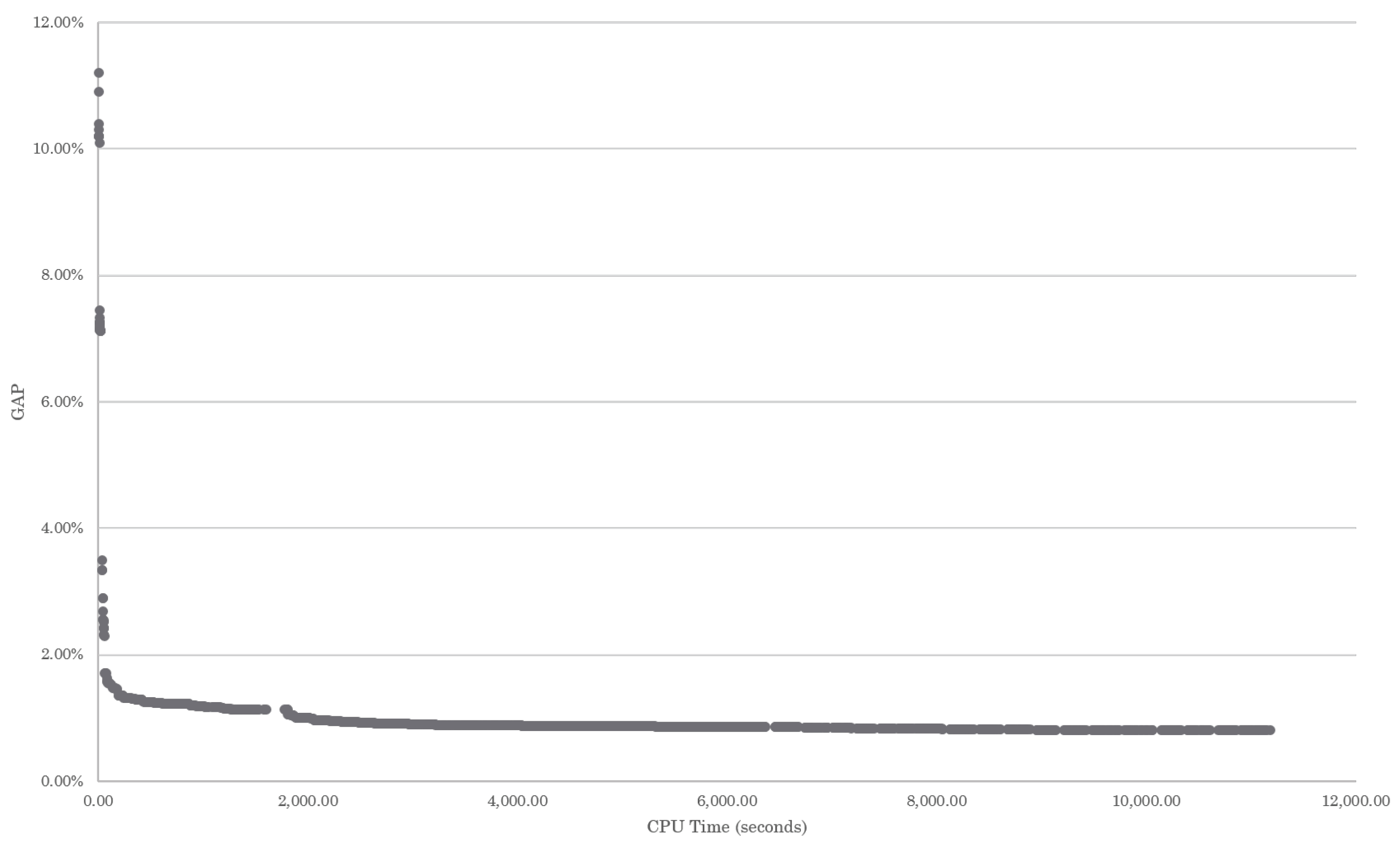
In particular, from the instances of 30 and 50 items, the formulation was unable to obtain optimal solutions; for those instances, we decided to increase the time limit of 7200 s imposed on the solver in pursuit of getting optimal solutions. However, the commercial solver got stuck in a positive GAP after more than 10,000 s. We analyzed the behaviour of the solver during the solution process on a test instance, evaluating the behaviour of the GAP when the elapsed time increased. Figure 1 illustrates this behaviour for Instance 30-1. Due to this, we decided to preserve the time limit of 7200 s for solving the case study.

Another point to highlight is that, for the instance of 50 items, the solution value was significantly higher than the rest of the cases. When revising in detail the cost segments contributing to the objective function, we realized that, for some cases, the model preferred to generate a high level of shortage, in particular for imported items. Based on this result, we could infer that the model determined when it was worth purchasing products or leaving a shortage in pursuit of minimizing costs. To validate this hypothesis, we conducted a complementary analysis by evaluating the case in which the formulation must fulfill the demand, through the WS model. The next section presents the results of this comparison.

4.4. Comparison between the AS Model and WS Model over Test Instances

The WS model was solved by the commercial solver CPLEX 12.9. The results obtained for the test instances are summarized in

Table 7. Performance of the WS model over the test random instances.

Instance	Objective Function	CPU Time (Seconds)
10-1	$528,137	0.688
10-2	$544,109	1.140
10-3	$595,973	0.625
10-4	$1,529,770	2.875
20-1	$1,008,150	0.813
20-2	$782,212	2.469
20-3	$1,120,920	0.750
20-4	$1,611,150	3.531
30-1	$1,447,230	3.969
30-2	$1,510,310	2.266
30-3	$1,340,600	3.515
30-4	$1,414,390	1.422
50-1	$4,015,590	1.953
50-2	$3,495,540	2.875
50-3	$4,135,130	2.953
50-4	$3,998,180	2.266
Average		2.220

. In this table, column 1 indicates the instance name, whereas columns 2, and 3 display the objective function and the elapsed CPU time, respectively.

As expected, the WS model solved all of the instances to optimality and produced higher objective function values than the AS model. In particular, the AS model obtained solutions that produced savings up to 35.80% of the objective function. However, we conducted a Man–Whitney analysis with a confidence level of 95 % to determine if the the savings were statistically significant. The alternative hypothesis ($H_a$), “the WS model computes higher objective function values than the AS model”, was evaluated against the null hypothesis ($H_o$) “there is no objective function value difference between the models”. The obtained p-value was 0.107, which accepted the null hypothesis that, eventually, both models could produce an equivalent total cost.

Another important aspect to analyze is the one related to the inventories. In this case, the inventory cost of the WS model was compared with the inventory cost plus the opportunity cost of the AS model. The results are displayed in

Table 8. Comparison between the total inventory costs for the model with and without shortage for the test random instances. IC, Inventory Cost; OC, Opportunity Cost; TC, Total Cost.

Instance	WS Model	AS Model			Monetary Savings	% of Savings AS vs. WS
	IC	IC	OC	TC
10-1	$266,897	$217,126	$33,570	$250,696	$16,111	6.04
10-2	$257,546	$214,408	$46,332	$260,740	$−3194	−1.24
10-3	$435,105	$408,633	$17,151	$425,784	$9321	2.14
10-4	$1,157,045	$1,100,163	$40,816	$1,140,979	$16,066	1.39
20-1	$455,757	$353,577	$76,390	$429,967	$25,790	5.66
20-2	$397,775	$358,129	$51,600	$409,729	$−11,955	−3.01
20-3	$770,110	$739,858	$40,505	$780,363	$−10,253	−1.33
20-4	$1,069,308	$996,489	$68,938	$1,065,427	$3880	0.36
30-1	$706,880	$635,984	$82,238	$717,922	$−11,042	−1.56
30-2	$815,893	$734,699	$84,400	$819,099	$−3205	−0.39
30-3	$638,094	$536,434	$119,413	$655,847	$−17,752	−2.78
30-4	$719,120	$660,574	$89,034	$749,658	$−30,537	−4.24
50-1	$3,042,402	$2,906,978	$3640	$2,910,619	$131,783	4.33
50-2	$2,697,426	$2,322,546	$2720	$2,325,267	$372,159	1.38
50-3	$2,886,510	$2,717,491	$4391	$2,721,882	$164,628	5.70
50-4	$2,953,503	$2,821,755	$2933	$2,824.688	$128,815	4.36

. For this table, column 1 displays the instance name, column 2 the Inventory Costs (IC) for the WS formulation, columns 3 and 4 the inventory cost, the Opportunity Cost (OC), and the Total Cost (TC) composed by the sum of the inventory cost and the opportunity cost (lost-sales costs), for the AS formulation, respectively. Column 6 estimates the savings gained by AS (monetary savings), and column 7 presents the percentage of savings of the AS model over the WS model (% of savings AS vs. WS). In the table, IC, OC, and TC are estimated by Equations (20), (21), and (22), respectively:

$$\begin{array}{ccc}\hfill IC& =& \sum _{i=1}^n\sum _{t=L{T}_{max}+1}^s{H}_i{I}_{it}\hfill \end{array}$$

(20)

$$\begin{array}{ccc}\hfill OC& =& \sum _{i=1}^n\sum _{t=L{T}_{max}+1}^s{P}_i{Z}_{it}\hfill \end{array}$$

(21)

$$\begin{array}{ccc}\hfill TC& =& IC+OC\hfill \end{array}$$

(22)

From Table 8, we observe that the AS model, in terms of inventory costs, was more cost effective than the WS model, producing savings up to 35.8%. However, the total cost, composed by the inventory and opportunity cost, presented a mixed behaviour, showing that 68.5% of the instances produced savings (values with a positive sign in the last column) when the AS model was compared with the WS model. We also observed that the WS approach produced higher values (up to 18%) of inventory costs than the AS model. Thus, the AS formulation could be useful to decrease the overstock while ensuring the availability of items (i.e., minimizing the shortage levels).

In particular, for the 20-3 instance and all 30 item instances, it was observed that the AS model produced an opportunity cost (estimated as the prices of the unsold items) that, after being added to the inventory cost, exceeded the inventory cost created by the WS model. The effect could be explained by the fact that, in order to minimize the final inventory, the AS model preferred to generate a high level of shortages in the last period, which was less expensive than buying complete batches that would be penalized at the end of the time horizon. However, in general, the AS model produced lower opportunity cost values, which also supported the fact that the model offered the advantage of determining which products should be prioritized at the time of purchase for each period.

In terms of CPU time, the WS model optimized the test instances within 4 s of CPU time, whereas for the AS model, the fastest instance required almost 9 s to solve to optimality. The results of the WS model could be used to obtain a “fast” purchasing plan in which all items will have overstock, and with the aim of minimizing the inventory levels, the company could create a clearance or sales strategy for the last period.

The inventory cost is commonly used to assess the efficiency of the overall purchase policy. We compared the final inventory costs of the two models. The results are reported in

Table 9. Comparison of the final inventory cost for the AS model and the WS model.

	Final Inventory Cost
Instance	WS Model	AS Model	% of Saving AS vs. WS
10-1	$3266.63	$888.88	72.57%
10-2	$3582.04	$238.48	93.34%
10-3	$2010.85	$11,153.38	42.64%
10-4	$4659.02	$700.67	84.96%
20-1	$6904.91	$1682	75.64%
20-2	$4809.59	$2362.96	50.83%
20-3	$4385.10	$1546.48	64.73%
20-4	$6772.98	$1680.18	75.19%
30-1	$9254.41	$1704.75	81.57%
30-2	$6180.20	$11,160.50	81.22%
30-3	$8781.33	$1885.40	78.52%
30-4	$8690.87	$2897.33	66.67%
50-1	$12,164.00	$3303.10	72.85%
50-2	$11,843.28	$4642.65	60.80%
50-3	$15,607.00	$4706.79	69.85%
50-4	$13,058.00	$4246.13	67.48%

. Column 1 shows the instance name and columns 2 ans 3 the final inventory cost for the WS model and the AS model, respectively. Column 4 shows the percentage of saving of the AS model over the WS model.

From Table 9, the AS model saved up to 93% of the final inventory cost computed in the WS model. Even when there was not significant evidence of savings with respect to the objective value against the AS model, a statistical analysis was conducted to determine if the AS model produced significant savings regarding the final inventory cost. We analyzed the results of the test instances by performing a hypothesis test. Given the distribution of the costs, a Mann–Whitney (non-parametric test) with a confidence level of 95 % was selected again for this purpose. The alternative hypothesis ($H_a$), “the WS model computes higher final inventory costs than the AS model”, was evaluated against the null hypothesis ($H_o$) “there is no final inventory cost difference between the models”. The test yielded a p-value of 0.013, which supported the evidence that the WS model computed higher final inventory costs than the AS model. However, the WS model reached the optimal results in a significantly shorter CPU time than the AS model. Based on these findings, we could conclude that the WS model could be used to determine the total cost for the worst scenario (i.e., avoiding shortages). In other words, by the WS model, it was possible to obtain an upper bound for the AS model.

4.5. Experimental Results over the Case Study

To conclude the present set of computational experiments, the performances of the WS and AS models were compared on real data provided by the company. Whereas the WS model solved this instance to optimality in 15.94 s, the AS model reached the time limit of 7200 s and reported a GAP of 0.81%. Regarding the objective function values,

Table 10. Comparison between the solution cost for the AS model and the WS model for the case study instance.

Objective Function		Monetary Savings	% of Savings AS vs. WS
WS Model	AS Model
$35,306,310	$29,532,400	$5,773,910	16.35

summarizes the results. In this table, columns 1 and 2 provide the objective function value obtained by the WS and AS models, respectively. Columns 3 and 4 display the savings of the AS model over the WS model, in monetary and percentage terms, respectively.

It is important to note that the AS model achieved significant monetary savings, which represented almost 17% of the total cost incurred by the WS model. In the real situation, these savings rose up to 33.33% with regard to the last year’s operation costs of the company (their costs according to our proposed objective function were equal to $44,078,209). For the case of the administration of the warehouse capacity, it could be observed that, according to the results of the $R_i$ variables, the AS formulation distributed the maximum inventories of the items in a way that the total stock in any period did not exceed 70% of the full capacity. In the case of the WS model, this value was not superior to 90%. Finally, the comparisons of the final inventory between both models is presented in

Table 11. Comparison between the final inventory cost for the AS and WS model for the case study instance.

	Final Inventory Cost
Instance	WS Model	AS Model	% of Savings AS vs. WS
Case study	$141,073	$36,201	74%

.

In the real situation, the company incurred a final inventory cost of $195,778.50. Therefore, both models improved this cost substantially. In particular, the AS model recovered approximately $32.29\%$ of the inventory cost, increasing the company’s profits by approximately $1.2\%$.

5. Conclusions and Future Work

This work addressed the capacitated lot sizing problem with lead times, batch ordering, and shortages. This problem was motivated by a retail company that sells clothes, shoes, and accessories by catalogue. The problem considered a retail environment in which items were not produced, but purchased from manufacturers (suppliers) who stipulated the batch ordering and who provided different delivery times (lead times) for each item. The problem was modelled and solved via an MILP formulation.

Two mathematical formulations were developed, one that allowed shortage (AS model) and another that did not (WS model). In the AS version, instances up to 20 items were solved to optimality, whereas the WS version solved all instances. The performance of the formulation was evaluated on different instance sizes. The AS model obtained significant savings (up to 17%) over the current situation of the company. Most relevantly, both mathematical formulations significantly improved the current situation of the company, saving up to 33% of the current final inventory costs. These results would be of interest to both academics and practitioners.

To assess whether introducing shortages benefited the company, we compared the final inventories computed by both models. The inventory costs in the AS version were cost-effective in all cases, but these savings were not statistically different from the savings gained in the WS model. In addition, the WS version optimized the test instances within 16 s of CPU time. In the case study, the best obtained solution deviated by 0.80% from the lower bound after reaching the specified time limit.

This research contributes to the body of knowledge as it optimized the CLSP by considering multiple items along with variable batch sizes and variable delivery times (lead times) in a retail environment. Still, the study addressed a comprehensive problem in the retail industry, but the approach assumed the following: first, there was a deterministic demand, which represented the first limitation of this study; and second, suppliers presented the right deliveries in terms of quality and amount and time, which represented the second limitation of this study. Any change to these assumptions would create a different scenario that should be addressed in a very particular way.

Further research should consider stochastic environments, in particular the uncertainty in the demand and/or lead times. Moreover, considerations such as the quality and timely deliveries by the suppliers can be questioned since these scenarios might not reflect 100% of the real-life cases. Including these variants will bring value to the lot sizing problem literature. Other considerations may include not only the lost-sales costs, but the cost of losing future customers in order to improve the estimation of opportunity costs. Finally, high-quality solutions within short computational time frames can be obtained by heuristics and metaheuristic algorithms. The models presented in this study will benefit companies by providing a good starting point to facilitate their decision-making process.