Bifurcations and Slow-Fast Analysis in a Cardiac Cell Model for Investigation of Early Afterdepolarizations


1
IUMA and Departamento Matemática Aplicada, University of Zaragoza, E-50009 Zaragoza, Spain
2
Departamento Matemáticas, University of Oviedo, E-33007 Oviedo, Spain
3
I3A, University of Zaragoza, IIS Aragón and CIBER-BBN, E-50018 Zaragoza, Spain
*
Author to whom correspondence should be addressed.
Mathematics 2020, 8(6), 880; https://doi.org/10.3390/math8060880
Submission received: 24 April 2020
/
Revised: 22 May 2020
/
Accepted: 23 May 2020
/
Published: 1 June 2020
(This article belongs to the Special Issue Mathematical Biology: Modeling, Analysis, and Simulations)
Abstract
:In this study, we teased out the dynamical mechanisms underlying the generation of arrhythmogenic early afterdepolarizations (EADs) in a three-variable model of a mammalian ventricular cell. Based on recently published studies, we consider a 1-fast, 2-slow variable decomposition of the system describing the cellular action potential. We use sweeping techniques, such as the spike-counting method, and bifurcation and continuation methods to identify parametric regions with EADs. We show the existence of isolas of periodic orbits organizing the different EAD patterns and we provide a preliminary classification of our fast–slow decomposition according to the involved dynamical phenomena. This investigation represents a basis for further studies into the organization of EAD patterns in the parameter space and the involved bifurcations.
Keywords:
cardiac dynamics; early afterdepolarizations (EADs); bifurcations; isolas; fast–slow decompositionMSC:
92B05; 34C23; 34C601. Introduction
In a healthy heart, the sinoatrial node sends out an electrical impulse, which spreads cell to cell throughout the heart, activating all cardiomyocytes to produce an electrical response called the action potential (AP). Upon being stimulated, cardiomyocytes in the lower chambers of the heart, the ventricles, suddenly increase their transmembrane voltage (depolarization). This increase is followed by a small partial voltage decrease (transient repolarization) and a prolonged plateau phase where voltage remains approximately constant. In the final part of the AP, transmembrane voltage decreases (repolarization) while returning to the resting potential level, which is maintained until receiving the next stimulus.
Under some circumstances, the normal sequence of AP phases can be reversed due to inward currents raising the transmembrane voltage during the plateau or repolarization phases of the AP, producing so-called phase-2 or phase-3 early afterdepolarizations (EADs). Drug side effects, ion channel dysfunction or oxidative stress, among others, can lead to the genesis of EADs [1,2,3]. In heart failure and genetic syndromes, EADs have been documented to be an important cause for lethal ventricular arrhythmias [4,5,6], but further knowledge is required to understand the mechanisms underlying EAD generation and the relationship between these cellular abnormalities and the occurrence of arrhythmias at tissue and whole-organ level that could eventually lead to sudden cardiac death.
Computational models of cardiac electrical activity have greatly contributed to shed light into varied cardiac phenomena, including EADs. Multiple models of mammalian ventricular cardiomyocytes have been used in the literature. Some of these are highly detailed, complex models with tens of state variables and hundreds of parameters, while there are other simpler models with just a few variables and parameters. Whereas complex (high-dimensional) models allow for greater realism in reproducing experimental observations and facilitating biophysical interpretation, simple (low-dimensional) models aid in isolating the dynamical mechanisms underlying a particular phenomenon and in performing a comprehensive theoretical study. In the present work, we use a low-dimensional approach based on a reduced three-variable cardiomyocyte model.
In 1991, Luo and Rudy [7] introduced a mathematical model of the membrane AP of a mammalian ventricular cell based on experimental data recently available at that time. This model, differently from subsequent models developed by the same authors, is called “passive” because all ionic concentrations, except for intracellular calcium, remain unchanged rather than varying dynamically over time. Due to its simple formulation and its ability to represent phenomena involving both depolarization and repolarization of ventricular cell, this model, either as such or with some simplifications, has been extensively used. In [8], a reduction in the number of variables of the Luo–Rudy model was proposed to investigate the mechanisms of EADs when decreasing the stimulation frequency. Initially, a model able to produce EADs was considered that contained three ionic currents, namely a fast current, an intermediate time-scale current, and a slow K current. Later, the fast current was discarded due to it having little effect on EAD generation, as it is activated mostly during the AP upstroke and is practically null during the plateau and repolarization AP phases. In our analysis, we use this reduced model to simplify the number of state variables at its maximum and, thus, facilitate a theoretical study.
From a mathematical point of view, this is a fast–slow dynamical system with multi-timescale phenomena. A fast–slow analysis of a reduced version of the Luo–Rudy model is presented in [8], considering a system with one slow and two or three fast variables. In that paper, the presence of a subcritical Poincaré–Andronov–Hopf bifurcation is shown as a signature of pseudo-plateau bursting. Similar analyses were published based on mathematical neuron models [9,10,11], where the classification of bursting models and the generation of new oscillations (spikes) were related, among others, with Poincaré–Andronov–Hopf and homoclinic bifurcations in the fast subsystem of two variables (dimension 2). While this approach has been successfully used in a variety of cardiac studies to investigate the causes for the presence or absence of EADs, it has recently been shown to fail in explaining the lack of certain types of EADs [12]. Considering the reduced three-variable version of the Luo–Rudy model presented in [8], a 1-fast, 2-slow decomposition is proposed [12,13] to provide more insight into the facilitation or inhibition of EADs as a function of the pacing frequency or pharmacological interventions. In this paper, we use this approach for the fast–slow decomposition and we characterize dynamical behaviors by introducing a sweeping technique, namely the spike-counting method. Besides, by using continuation techniques, we describe some bifurcations of the system and we show, for the first time to the best of our knowledge, the presence of isolas of families of periodic orbits in the reduced Luo–Rudy model.
The paper is organized as follows. In Section 2, the reduced model used to describe the electrical behavior of a mammalian ventricular cardiomyocyte is presented. In Section 3, the dynamical analysis performed to identify parametric regions with EADs and generate associated bifurcation diagrams is described. In Section 4, the discussion and conclusions of the study as well as recapitulating classification figures regarding EAD generation are presented.
2. The Reduced Luo–Rudy Mammalian Ventricular Cell Model
Following a Hodgkin and Huxley formalism [14], Luo and Rudy proposed a mathematical model of a mammalian ventricular cell (LR91) [7]. The rate of change of the transmembrane potential (V) is given by
where is the membrane capacitance, in this study set at , as in [13], and subsequently varied to investigate its role in facilitating the generation of EADs. In the above equation, is an external stimulus current and is the sum of the ionic currents in the cell. All ionic currents were computed for a membrane area of . Six ionic currents were defined in the LR91 model: , a fast sodium current; , a slow inward current; , a time-dependent potassium current; , a time-independent potassium current; , a plateau potassium current; and , a time-independent background current.
Since here we focus on EAD generation, we follow the approach proposed in [8] and we discard the fast current for the reduced version of the LR91 model. Although some studies have described a role for the sodium current in the generation of EADs [2,3], it should be noted that this current has two components, namely the fast sodium current and the late sodium current. While the late sodium current flows throughout the AP plateau and its involvement in EAD generation has been well documented, the fast sodium current contributes to the AP depolarization and has a more limited contribution to EADs. In the reduced model used in this work, only the fast sodium current is included and, thus, we discard it based on its reduced contribution to the investigated phenomenon. The other two ionic currents in the reduced model are: , which is a calcium current with an activation gating variable d and an inactivation gating variable f; and , which is a time-dependent potassium current with a time-dependent activation gating variable x and a time-independent inactivation gating variable set to one for simplification. The reversal potential of calcium was set at , rather than being time-dependent as in the LR91 model.
The values of the gating variables used to define the ionic currents are obtained as the solution of a coupled system of nonlinear ordinary differential equations (ODEs) of the form , where y represents any gating variable, is its time constant, and is the steady-state value of y [7].
An additional simplification to the four-variable system (V, d, f, and x) proposed in [8] was later described by Kügler [15]. The gating variable d was replaced with its steady-state function and the time-constant functions and were assumed to be constant, thus being represented by and .
With all these simplifications, the three-variable model used here [12] was described by the following ODE system:
with the inward ionic calcium current (with the calcium channel conductance and the dynamic inactivation variable f) and the outward ionic potassium current (with the potassium channel conductance and the dynamic activation variable x) defined by:
The steady-state functions were given by:
The fixed parameter values used in this study, unless otherwise stated, were:
It should to be noted that, whereas the LR91 model well represents the behavior of a ventricular cardiomyocyte with constant resting membrane potential during Phase 4, the reduced model described above presents a Phase 4 with slowly increasing transmembrane potential. Thus, an external stimulus is required to depolarize the AP in the LR91 model, but the AP depolarizes spontaneously when transmembrane potential reaches a threshold in the case of the reduced model. Consequently, in the above equations for the three-variable model.
3. Dynamical Study
We showed that the reduced version of the LR91 model described above presents a behavior comparable to that of typical spiking-bursting activity [9,10,11]. To achieve a better understanding of the model dynamics, we performed a detailed numerical analysis using both a spike-counting technique and numerical continuation to detect the main bifurcations. Numerical simulations were performed using a variable-stepsize variable-order Taylor series method (software TIDES (https://sourceforge.net/projects/tidesodes/) [16,17]), which provides a highly accurate numerical ODE solver, using as error tolerance.
3.1. Spike-Counting Sweeping
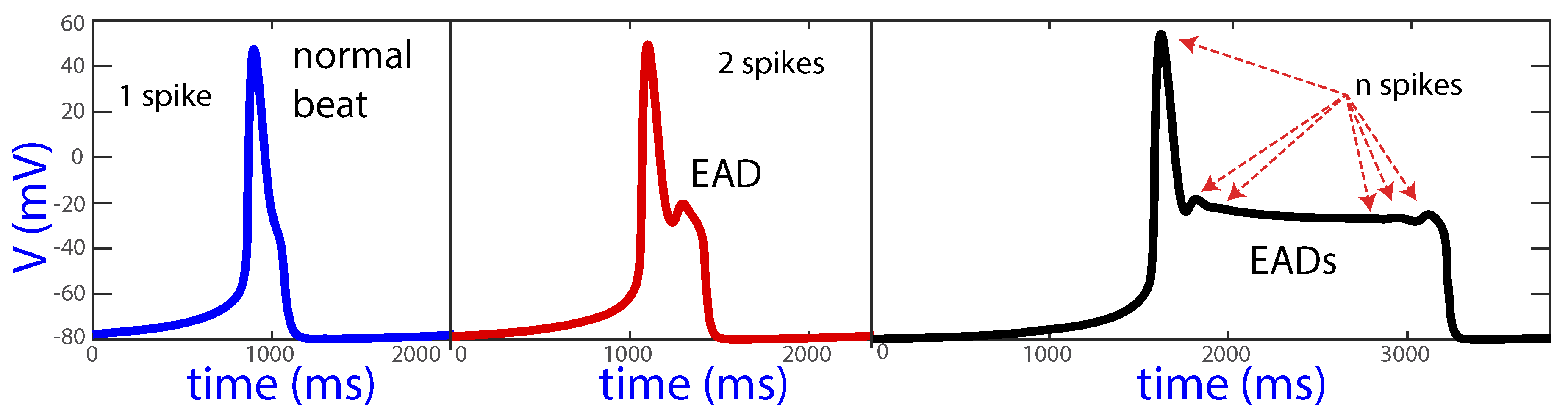
When EADs are generated, extra spikes can be seen in the plateau of the AP. Figure 1 shows a normal beat with no EADs, a beat with one EAD and a beat with several EADs (more than 2 spikes).
The spike-counting technique consists of detecting the number of spikes of the limit cycles of the system, when these exist [18]. Regions of parameter values with the same number of spikes per beat are represented with the same color. This allows appreciating different bands in the parameter space, which characterize the structure of the model. The detection of the number of spikes per orbit is performed by computing all relative maxima and minima and by counting the spikes where the relative difference between the maxima and minima in the voltage variable is higher than a threshold. Here, the threshold is set at so as not to include very small oscillations that occur in action potentials such as the one represented on the right panel of Figure 1. The number of counted spikes is clearly sensitive to the selection of the threshold value, but the global behavior in terms of the occurrence of EADs is generally well captured, as all main voltage changes during the AP plateau are detected.
In our analysis, we used the conductances of the calcium and potassium currents, and , as the main set of parameters to investigate their involvement in EAD occurrence. We also investigated variations in the cell capacitance, . This represents a further step from previous studies that considered variations only in [8] or both and [12] to determine the presence of EADs. While using a reduced model facilitates theoretical understanding on the mechanisms for EAD generation, future works should be conducted with more complex and more realistic cardiomyocyte models that allow meaningful interpretations regarding the parameters involved in the occurrence of EADs.
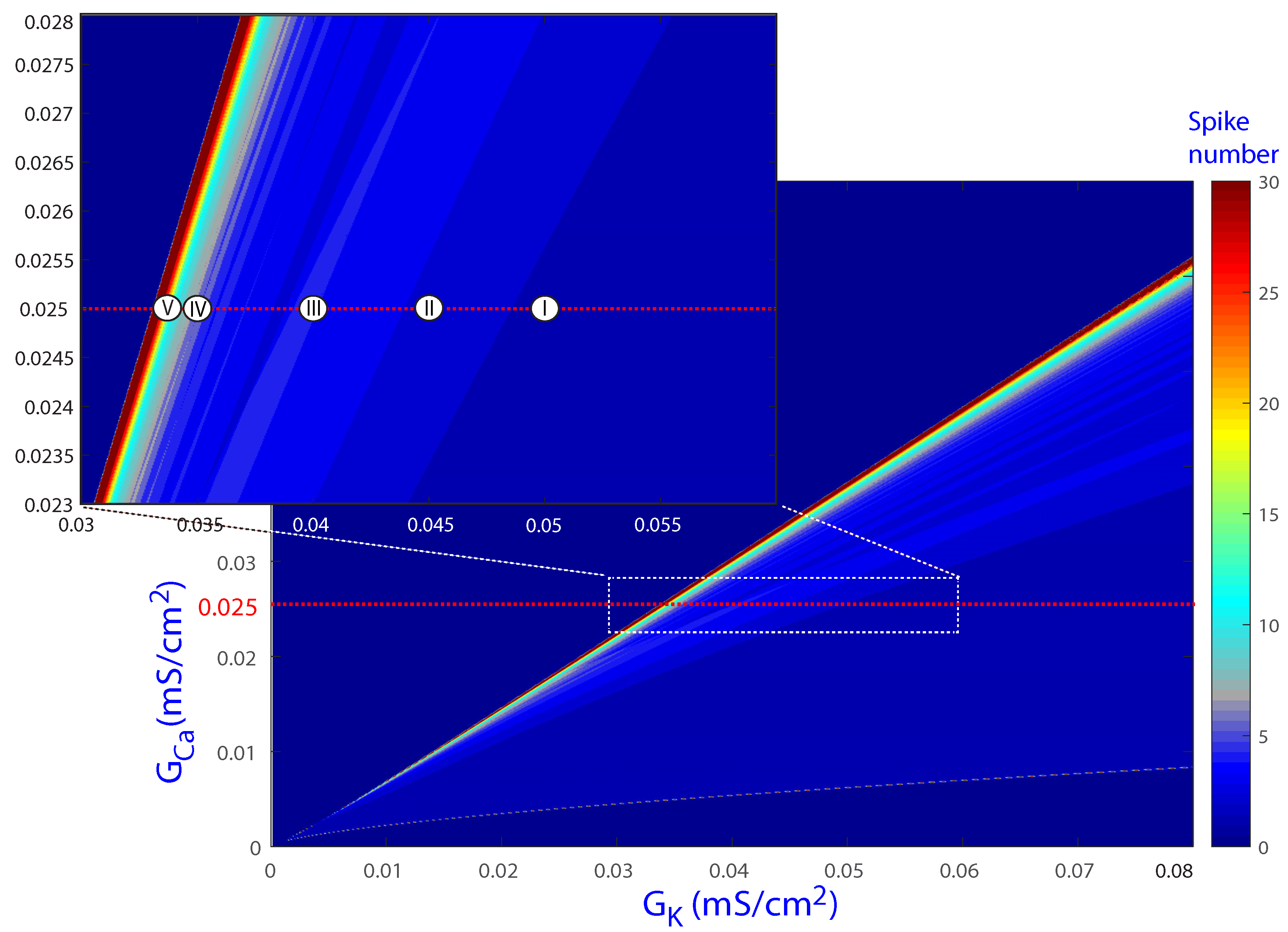
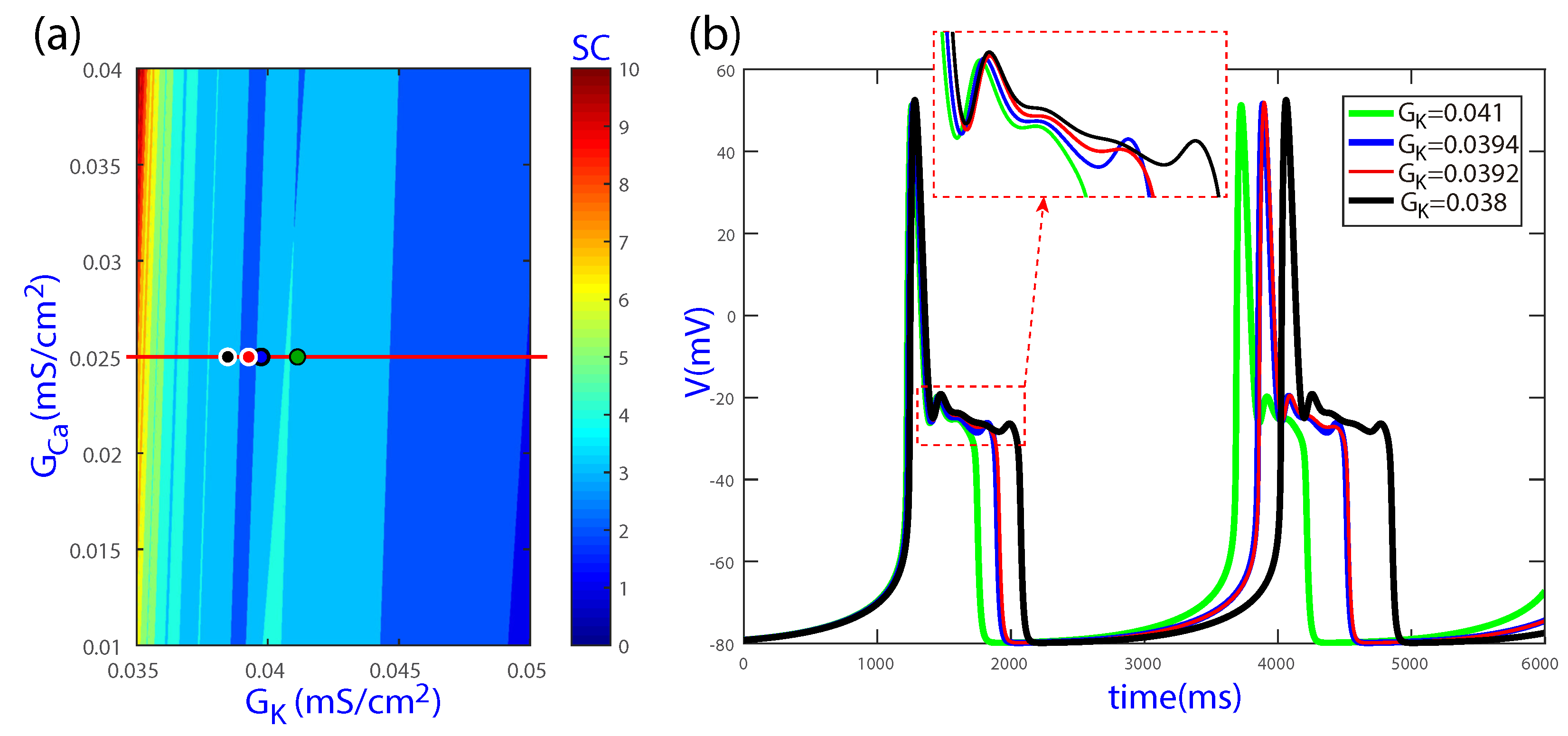
Figure 2 shows the results of the spike-counting technique for the biparametric plane (, ), with the upper left inset presenting a magnification of a specific area. Colors indicate different cellular behaviors. Darkest blue denotes cases where no beats are generated. Slightly lighter blue corresponds to normal beats without EADs, an example of which is illustrated in Figure 3b for the parameter values of Point I. In the region of Point II, the periodic orbit shows one EAD, as exemplified in Figure 3d. When the parameters move to the lightest blue and red regions, more EADs are present, as shown in Figure 3f for Point III and in Figure 4c,f for Points IV and V, respectively. In particular, Point III corresponds to the default values and , for which EADs are present. Based on the different cellular behaviors indicated by the color band structure in Figure 2, further analyses were performed for the default value of while varying along the horizontal red line, as described in the following sections.
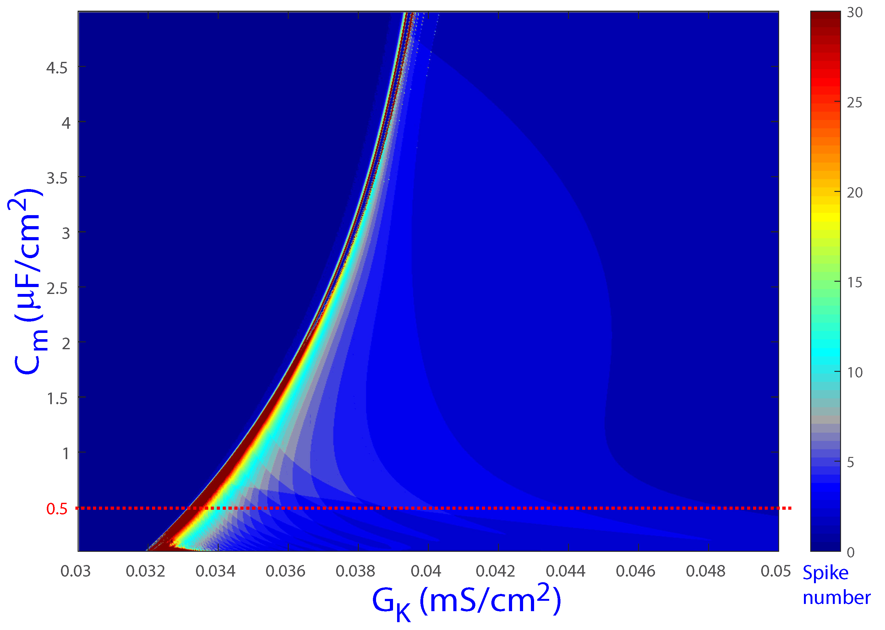
Figure 5 shows additional spike-counting results for the biparametric (, ) plane, with the horizontal red line corresponding to the default value (and ). In this case as well, color bands can be observed, rendering similar structures to those shown for the (, ) plane in Figure 2. Based on the results shown in the two figures, bounded regions in the global parameter space can be expected in the characterization of EAD dynamics.
3.2. Fast–Slow Analysis
The reduced version of the LR91 model used in this study is a fast–slow system, since its state variables change at different time scales. When analyzing a fast–slow system, it is of major relevance to investigate the bifurcation diagrams of the limit cases (when the parameters responsible for the difference in time scales are considered to be zero) [10]. This approach uses geometric singular perturbation methods and allows (partially) explaining the dynamics when such parameters are small enough (see [19] for a review and [9] for the basic theory and for classification of bursting mechanisms).
The default values of the time constant parameters characterizing the state variables f and x in the reduced LR91 model are and . An estimate of the time constant for the state variable V can be obtained by [12]. This means that V is the fastest state variable and x is the slowest one, while the state variable f can be considered as a fast or a slow one. In [8], the four-variable (V, d, f, and x) system was decomposed into a fast three-variable (V, d, and f) subsystem and a slow one-variable (x) subsystem, thus including f as a fast variable. In [15], a simpler three-variable (V, f, x) model was considered, as d was replaced with its steady-state function . The fast subsystem was defined to contain two variables (V and f), thus again taking f as a fast state variable. On this basis, a fast two-variable and a slow one-variable subsystems were analyzed and their information was combined to characterize the dynamics of the full three-variable system. By fixing x, the model analysis provides two invariant objects: a curve of equilibrium points and a manifold of limit cycles. The main issue with this approach is that it does not explain some changes in the system, as illustrated in [12]. To solve this issue, some studies have decomposed the same three-variable system into a fast one-variable (V) and a slow two-variable (f and x) subsystems [12,13]. A systematic analysis of the geometric singular perturbation methods for 1-fast, 2-slow variables is given in [20,21].
In this study, we considered, on the one hand, the reduced LR91 model (Equation (1)) using the fast time scale :
where is a parameter that takes small values () and , as no external stimulus was considered (), as in [12,13]. When decreases to zero (), the system described in Equation (3) defines orbits that converge during fast dynamics to solutions of the fast subsystem or layer equations given by:
On the other hand, when the orbits have slow dynamics, the fast variable moves so rapidly that it can be considered to have already reached steady-state. Thus, changing to the time scale and taking the limit case, the orbits converge to solutions of the differential algebraic equation (DAE) system, called the slow-flow system, given by:
The solutions of Equation (5) evolve on the manifold given by , which is called the critical manifold and is denoted by . Besides, this gives the manifold where the equilibria of the fast subsystem are. It follows from Fenichel theory [22] that this manifold perturbs to invariant manifolds that exist for small enough in the full system.
In the following, a detailed investigation of the geometry of the bursting orbit dynamics for the reduced LR91 model, and in particular the orbits for the set of parameters corresponding to Points I–V in Figure 2, is performed. Taking the model equations defined by Equation (1), the critical manifold is given by the cubic-shaped surface:
Figure 3 shows the outer sheets of the surface, which are attracting ones, and the middle sheet, which is a repelling one. The different sheets are separated by curves corresponding to fold bifurcations of the fast subsystem:
From the analysis of limit cases and Fenichel theory, the solutions of the global system were found to evolve in the slow epochs close to one of the attracting sheets of the critical manifold. The evolution on the attracting sheets was found to give the stable hyperpolarized and stable depolarized steady-states. Close to the fold bifurcations, the orbits quickly fell down to the other attracting sheet. The rapid transitions between the attracting sheets were approximated by solutions of the fast one-variable subsystem in Equation (4).
As described above, the equations of the slow motion on the critical manifold are given by Equation (5), where differential equations describe the motions of the variables f and x, whereas the fast variable V is implicitly described by the first algebraic equation in Equation (5). Through several manipulations (see [12,13,19] for details), the slow subsystem can be transformed into the so-called desingularized system:
Folded singularities are equilibria of the desingularized system only, but not of the slow subsystem in Equation (5) or the initial model in Equation (1). Thus, they lie on a fold curve and satisfy:
A study of their linear stability suggested they are folded-node equilibria in this system. These special points give a route to the solutions of the slow subsystem to cross the folds from an attracting sheet and to move some time on the repelling sheet. Therefore, these points may generate the so-called singular canards (see [19,23] for details).
The existence of canard orbits have relevant consequences in many different systems, as they allow uncovering mechanisms of sudden changes. For instance, they were linked to the spike-adding phenomena in the Hindmarsh-Rose neuron model [24,25]. In a reduced LR91 model, canard orbits were shown to organize the first EADs generated on the orbits in phase space [12]. This is well explained in references [12,13] and therefore here we focus on the different geometric characterizations of the periodic orbits of the system showing where EADs are produced by the canard orbits and where different phenomena are also present.
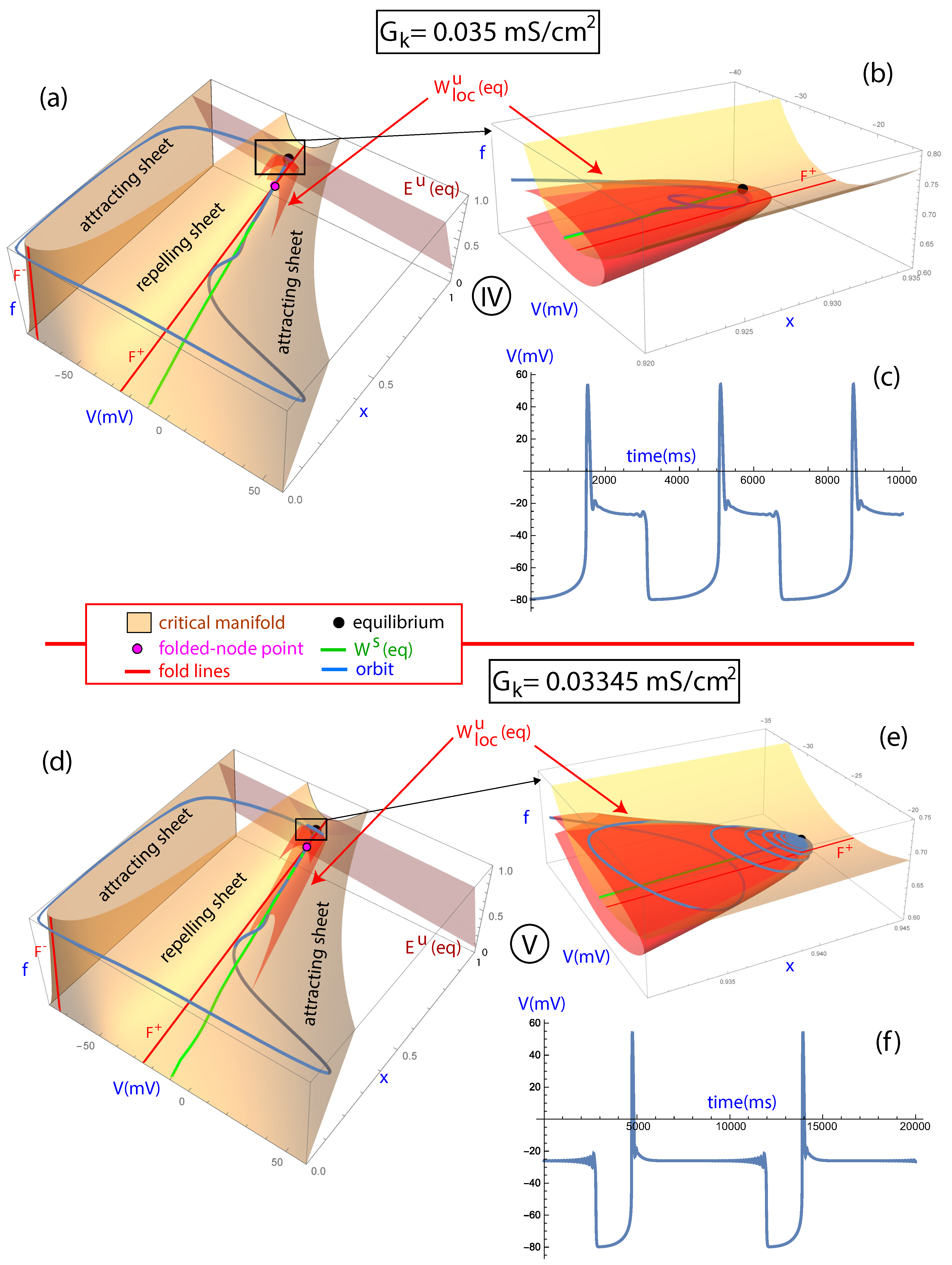
In Figure 3, the fast–slow geometry is described for the orbits with labels I, II, and III in Figure 2 on the parametric line . The critical manifold is shown in orange, with the attracting and repelling sheets separated by the fold lines, and , in red and with the periodic orbits in blue. The temporal evolution of the variable V of the periodic orbit is shown on the right panels. It can be observed that in Case I for the orbit presents a normal beat without any EADs (Figure 3a,b). In this case, the orbit presents the “nominal behavior”, remaining most of the time on the critical manifold of the slow motion and fast transitioning between the attracting sheets close to the fold lines. Note that the orbit is far from the folded-node singular point in magenta and, therefore, there is no canard orbit. By moving forward on the line towards Point II corresponding to , it can be observed that the orbit has one EAD (Figure 3c,d). In this case, the orbit passes near the folded-node singular point and this allows the orbit to make a loop on the repelling sheet before progressing to the other attracting sheet (see [13]). By further moving on the parametric line towards Point III corresponding to , more EADs are generated by the maximal canards (Figure 3e,f). Maximal canards are given by the intersections of the depolarized attracting and the repelling sheets of the slow manifold of the system and extended by the flow (for more details, see [12,13,26]). The equilibrium point, which is a saddle-node of type (1,2) with eigenvalues , , and , is attracting the orbit along the stable manifold of the equilibrium (in green) at the same time that the canard orbits generate new EADs until the orbit progresses to the other attracting sheet (see inset in Figure 3e). This phenomenon has been previously observed in other 1-fast, 2-slow variables systems [27,28,29].
Figure 4 shows how further variations in the bifurcation parameter lead to higher numbers of EADs as the orbit approaches the equilibrium point shown in black. The two orbits presented in Figure 4 contain a large number of EADs, particularly the second one. The mathematical mechanism explaining such a large number of EADs is twofold: the described canard phenomenon that gives rise to EADs when the orbit passes near the folded-node and the stable manifold of the equilibrium that increasingly pulls the orbit closer to that point. On the orbit of Point IV corresponding to , there is a saddle-focus equilibria of type (1, 2) with eigenvalues , , and . It can be observed in Figure 4 how such an orbit oscillates due to the canard orbits around the stable manifold of the equilibria until reaching a point close to the equilibrium point (Figure 4a,b). Consequently, the orbit remains more time active as the orbit approaches the equilibrium and it subsequently spirals outward (last spikes of the orbit). This can be appreciated in the two-dimensional local unstable manifold of the equilibrium shown in Figure 4. In a previous study, this phenomenon was observed as a first approximation using the unstable linear subspace of the equilibrium [15]. In addition, similar observations hold for the last investigated point, i.e., Point V corresponding to (Figure 4d,e). As before, the first oscillations are due to the canard phenomena and the fact of passing near the folded-node singularity, while subsequent oscillations can be explained by the orbit approaching the saddle-focus equilibria of type (1,2) with eigenvalues , and . It can be noted that in this case the ratio , which makes the attracting dynamics strong and prolongs the approach towards the equilibrium point. When the orbit is already close enough to the equilibrium point, the unstable manifold takes control of its escape dynamics and the orbit follows this manifold. This is illustrated in the inset of Figure 4d, which shows how the orbit spirals the two-dimensional local unstable manifold . The small variations in the plateau phase of the AP closely resemble the oscillations present in pseudo-plateau bursting, whose dynamics has also been studied for 1-fast, 2-slow variables systems [21].
As the parameter takes decreasing values, the orbit approaches more and more the saddle-focus equilibria. As shown above, more and more small spikes are then generated. The fact of setting a threshold on voltage when counting the number of spikes may render the algorithm unable to detect a small spike, as shown in Figure 6, which can be additionally influenced by the enlargement of the orbit approaching the saddle-focus equilibria. This may generate transitions between areas of different colors, which would seem to indicate a change in the number of spikes by one or more spikes even if this is not actually the case.
3.3. Isolas of Periodic Orbits
To investigate bifurcations on the parametric line , numerical analysis with continuation techniques was performed using the software AUTO [30,31]. The main focus of this study was to explore the presence of isolas of periodic orbits, that is, simple closed curves of families of periodic orbits. These isolas have been described for other models, such as the Koper model of chemical reactions with mixed-mode oscillations (see Figure 19 in [19]). For the reduced LR91 model used in this study, some bifurcations are identified in [12] but no isolas are shown.
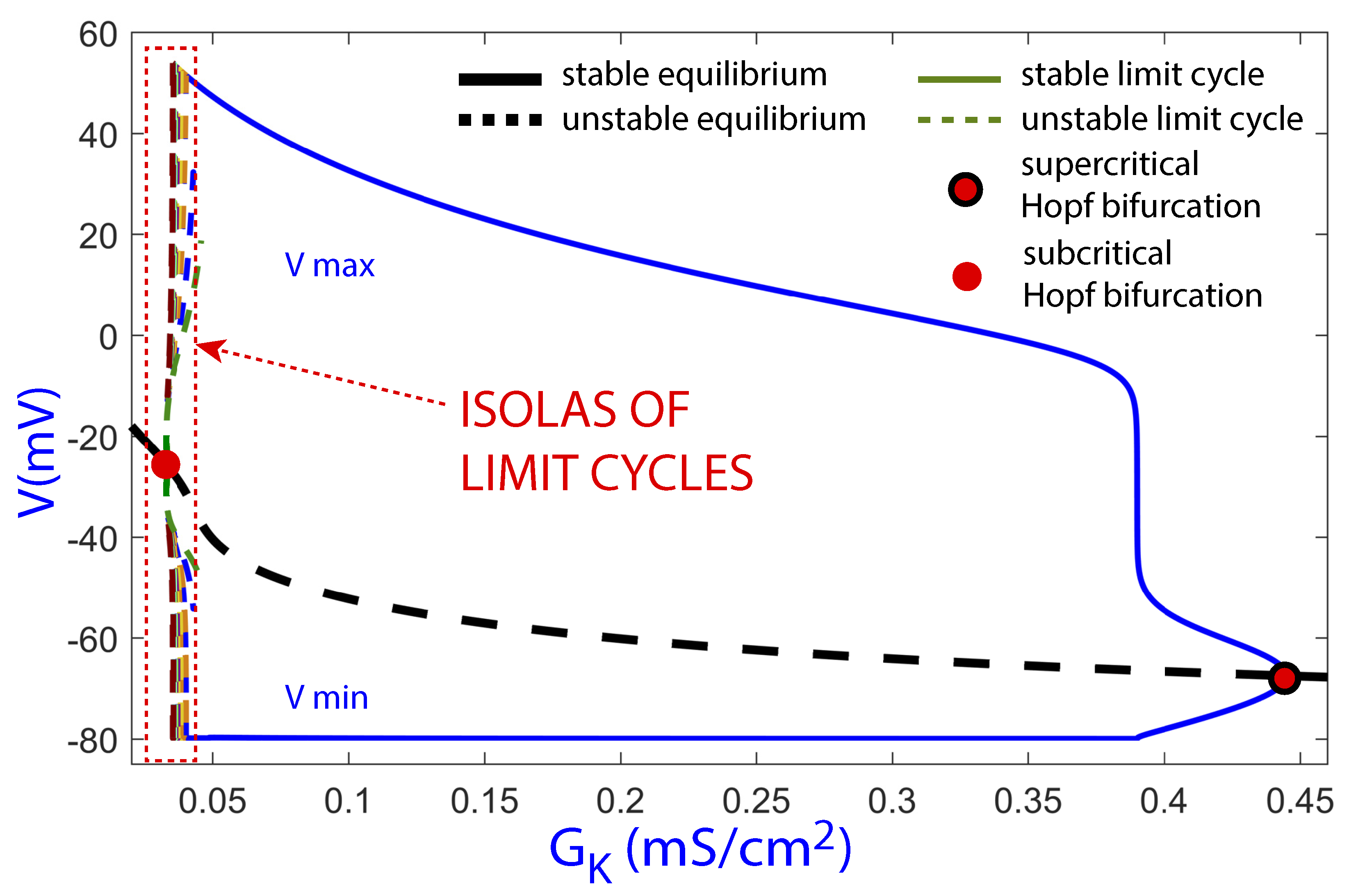
Figure 7 shows the bifurcation diagram obtained with the software AUTO using as the continuation parameter on the line . The bifurcation diagram shows the maximum (the highest peak of the orbit) and minimum (resting membrane potential) values of the transmembrane voltage variable V for different periodic orbits corresponding to a range of given values of the continuation parameter. The continuation of the equilibria (black thick line) and limit cycles (color lines) are shown too. Continuous lines are stable invariants while discontinuous lines are unstable ones. In the figure, presenting a large parametric interval , two Poincaré–Andronov–Hopf bifurcations can be observed, a subcritical one on the left part and a supercritical one on the right part. As decreases, the stable periodic orbits generated at the supercritical Hopf bifurcation move to the left towards the subinterval for with associated EADs.
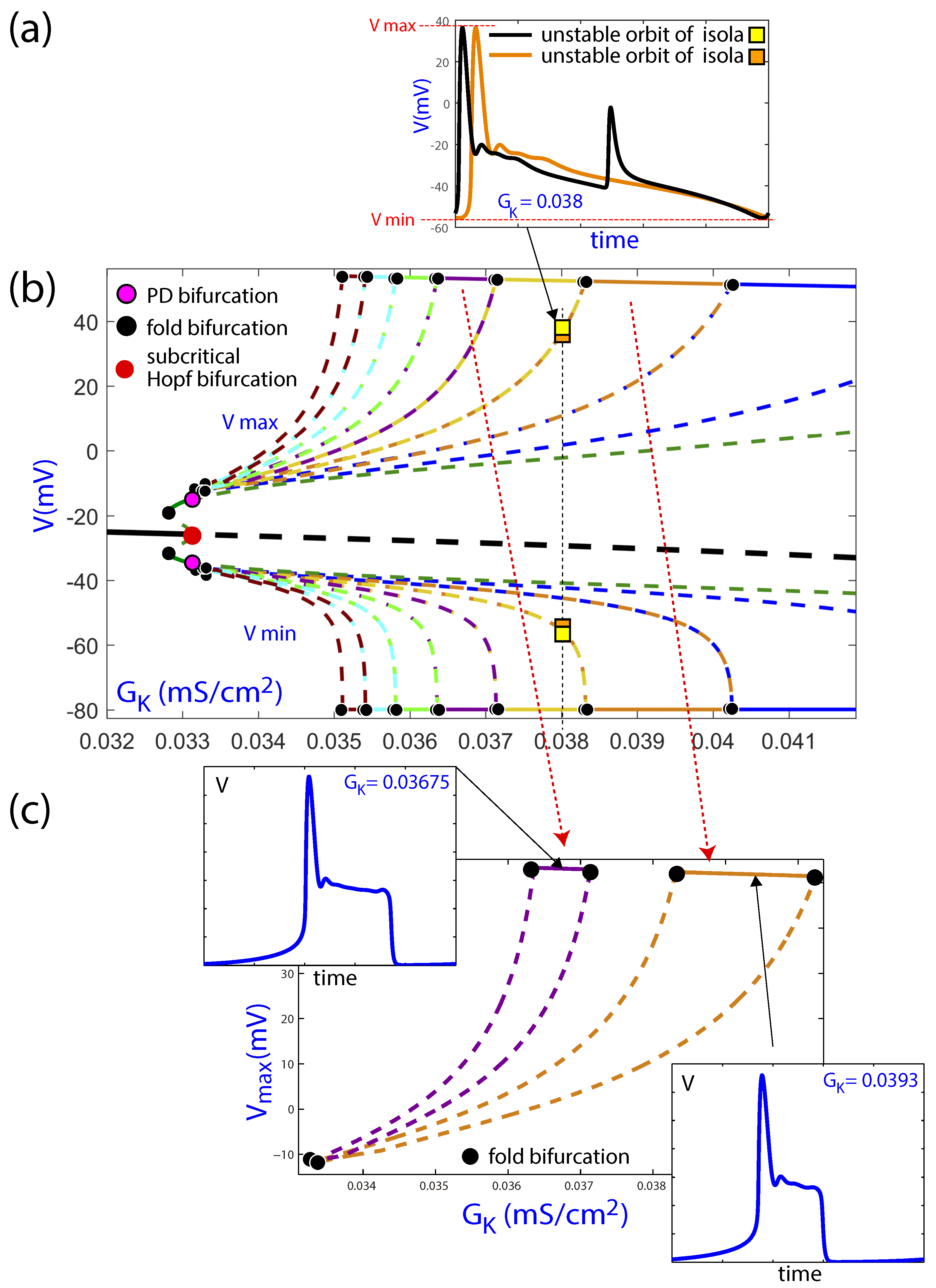
In the subinterval with several EADs, shown in Figure 8b, families of periodic orbits can be observed, which are plotted in different colors. These families are organized in isolas, that is, closed family curves of periodic orbits with different numbers of oscillations in the form of EADs. The different isolas have a section formed by stable limit cycles placed mainly on the top (and bottom, as it is the maxima and minima) of the isola. These stable periodic orbits lose their stability at fold bifurcations (or saddle-node bifurcations of limit cycles), as indicated in [12]. However, the stable line is in fact a discontinuous one, as it is formed by the top subintervals of stable periodic orbits of the different isolas, and not a continuous line with several bifurcations. The unstable parts of the isolas shown in the figure evolve with similar maximum and minimum values, which explains why they are so closely represented in Figure 8b, while they are formed by different limit cycles, as can be appreciated in Figure 8a. Besides, there are fold and period-doubling bifurcations on the bifurcated periodic orbits from the subcritical Hopf bifurcation.
Two of the isolas in Figure 8b are represented separately in Figure 8c only for the maximum value of voltage. Now, the fold bifurcations are clearly seen as the limit of the stable periodic orbits. The temporal evolution of voltage along the hearbeat is represented for the two parametric values marked with a black dot in each of the two isolas, each showing a different number of EADs. The stable part of the isolas is located on the flat top segment, which corresponds to the observed limit cycles. These results confirm that the reduced LR91 model exhibits isolas of periodic orbits, as reported for other fast–slow models in the literature [19]. This can be the basis for further studies into the organization of EAD patterns in the parameter space and the involved bifurcations.
4. Discussion, Conclusions, and Future Work
In this study, we investigated the dynamical mechanisms for EAD generation in the reduced LR91 mammalian ventricular cell model. As in recent studies [12,13], we considered a fast–slow decomposition of the system with 1-fast and 2-slow variables rather than 2-fast and 1-slow variables [8], and we analyzed the influence of maximal canard orbits. We used sweeping techniques (the spike-counting method) as well as continuation techniques. The former allowed us to identify different parametric regions with EADs (see a summary in Figure 9), whereas the latter was used to generate bifurcation diagrams for the mentioned parametric regions. We showed the existence of isolas of periodic orbits and we performed a preliminary classification of the fast–slow decomposition in various cases according to the involved dynamical phenomena.
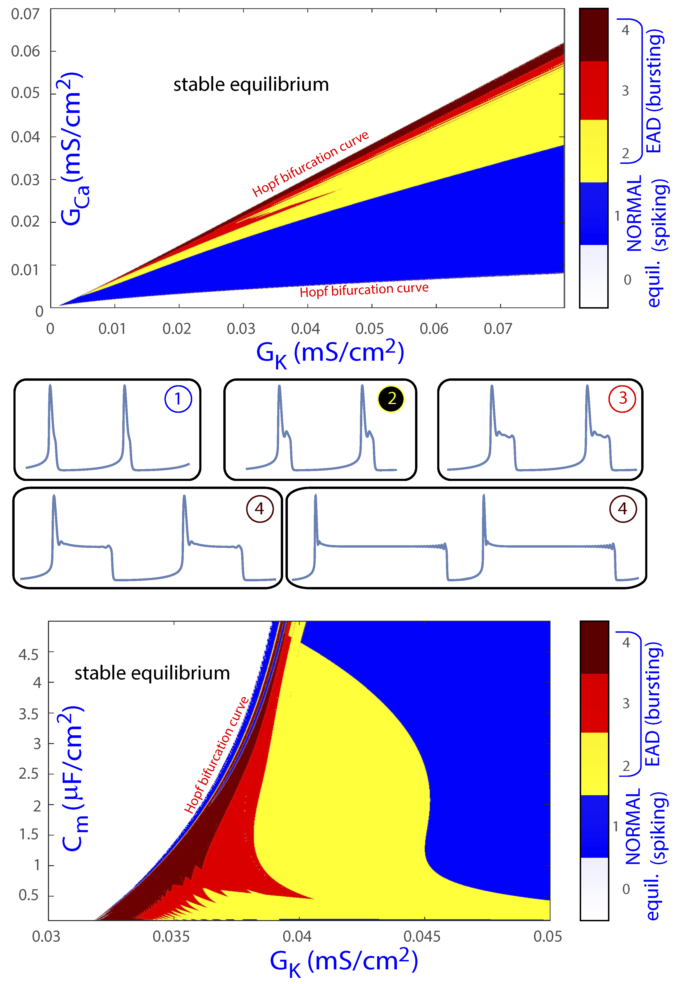
As a summary, based on the dynamics on the critical manifold and near the unstable equilibrium point, several regions in the (, ) and (, ) parametric planes associated with different dynamical behaviors can be identified. Specifically, regarding EADs, the first region corresponds to cases where the orbit has an EAD due to a maximal canard orbit. As more canards take part in the process, more EADs are generated. When the orbit approaches the equilibrium, this gives rise to additional oscillations. When the equilibrium point is of saddle-focus type, the orbit gets closer and closer to the equilibrium and spirals following its unstable manifold. These mechanisms create EADs corresponding to small oscillations of voltage during the course of the AP, commonly in association with AP prolongation. Figure 9 recapitulates our classification of the dynamical behaviors of the orbits in the (, ) and (, ) parametric planes: white is associated with no activity, that is, the equilibria is an attractor; blue corresponds to normal beats; yellow denotes EADs created by the maximal canards; red corresponds to the attracting behavior of the equilibria on the stable manifold direction with AP prolongation; and maroon is for very elongated APs remaining close to the saddle-focus equilibria. Color regions, associated with active cell status, are delimited by two Hopf bifurcations that make the equilibrium point unstable in the middle parametric interval. As can be noted from the two panels in Figure 9, results for both (, ) and (, ) parametric planes render bands that allow making a parametric description of the areas in the parameter space that lead to EAD generation. This sets the basis to investigate actions able to move the system, i.e., the mammalian ventricular cell, to parameter regions far from areas prone to arrhythmogenic EADs. Part of our future research in this line focuses on studying the effects of including an external stimulus in this model and the dynamics of other, more complex and realistic cardiomyocyte models. This would allow more meaningful interpretations regarding the parameters involved in the occurrence of EAD.
Author Contributions
Conceptualization, R.B.; software, R.B. and L.P.; formal analysis, R.B., M.A.M., L.P., and E.P.; writing—original draft preparation, R.B. and M.A.M.; and writing—review and editing, R.B., M.A.M., L.P., and E.P. All authors have read and agreed to the published version of the manuscript.
Funding
R.B. and M.A.M. have been supported by the European Social Fund (EU), Aragón Government (Grant LMP124-18 and Group E24-17R), and the University of Zaragoza-CUD (grant UZCUD2019-CIE-04). R.B. has been supported by the Spanish Ministry of Economy and Competitiveness (grant PGC2018-096026-B-I00). M.A.M. has been supported by the Spanish Ministry of Economy and Competitiveness (grant DPI2016-75458-R). L.P. has been supported by the Spanish Ministry of Economy and Competitiveness (grant MTM2017-87697-P) and by Programa de Ayudas “Severo Ochoa” of Principado de Asturias (Grant PA-18-PF-BP17-072). E.P. has been supported by the European Research Council (Grant ERC-638284), Spanish Ministry of Economy and Competitiveness (grant DPI2016-75458-R), European Social Fund (EU), and Aragón Government (grant LMP124-18 and Group T39-17).
Conflicts of Interest
The authors declare no conflict of interest.
Abbreviations
The following abbreviations are used in this manuscript:
| EADs | Early AfterDepolatizations |
| LR91 | Luo–Rudy model (1991) |
| AP | Action Potential |
References
- January, C.T.; Riddle, J.M. Early afterdepolarizations: Mechanism of induction and block. A role for L-type Ca2+ current. Circ. Res. 1989, 64, 977–990. [Google Scholar] [CrossRef] [PubMed] [Green Version]
- Song, Y.; Shryock, J.; Belardinelli, L. An increase of late sodium current induces delayed afterdepolarizations and sustained triggered activity in atrial myocytes. Am. J. Physiol. Heart and Circ. Physiol. 2008, 294, 2031–2039. [Google Scholar] [CrossRef] [PubMed] [Green Version]
- Xie, L.; Chen, F.; Karagueuzian, H.; Weiss, J. Oxidative-stress-induced afterdepolarizations and calmodulin kinase II signaling. Circ. Res. 2008, 104, 79–86. [Google Scholar] [CrossRef]
- Antzelevitch, C.; Sicouri, S. Clinical Relevance of Cardiac Arrhythmias Generated by Afterdepolarizations. Role of M Cells in the Generation of U Waves, Triggered Activity and Torsade De Pointes. J. Am. Coll. Cardiol. 1994, 23, 259–277. [Google Scholar] [CrossRef] [Green Version]
- Huffaker, R.B.; Weiss, J.N.; Kogan, B. Effects of early afterdepolarizations on reentry in cardiac tissue: A simulation study. Am. J. Physiol. Heart Circ. Physiol. 2006, 292, 3089–3102. [Google Scholar] [CrossRef]
- Sato, D.; Xie, L.H.; Sovari, A.A.; Tran, D.X.; Morita, N.; Xie, F.; Karagueuzian, H.; Garfinkel, A.; Weiss, J.N.; Qu, Z. Synchronization of chaotic early afterdepolarizations in the genesis of cardiac arrhythmias. Proc. Natl. Acad. Sci. USA 2009, 106, 2983–2988. [Google Scholar] [CrossRef] [Green Version]
- Luo, C.; Rudy, Y. A model of the ventricular cardiac action potential. Depolarization, repolarization, and their interaction. Circ. Res. 1991, 68, 1501–1526. [Google Scholar] [CrossRef] [Green Version]
- Tran, D.X.; Sato, D.; Yochelis, A.; Weiss, J.N.; Garfinkel, A.; Qu, Z. Bifurcation and Chaos in a Model of Cardiac Early Afterdepolarizations. Phys. Rev. Lett. 2009, 102, 258103. [Google Scholar] [CrossRef] [Green Version]
- Rinzel, J. A Formal Classification of Bursting Mechanisms in Excitable Systems. In Mathematical Topics in Population Biology, Morphogenesis and Neurosciences, Proceedings of the International Symposium, Kyoto, Japan, 10–15 November 1985; Teramoto, E., Yumaguti, M., Eds.; Springer: Berlin/Heidelberg, Germany, 1987; pp. 267–281. [Google Scholar]
- Ermentrout, G.B.; Terman, D.H. Mathematical Foundations of Neuroscience; Springer: New York, NY, USA, 2010; Volume 35. [Google Scholar]
- Barrio, R.; Martínez, M.A.; Serrano, S.; Shilnikov, A. Macro- and micro-chaotic structures in the Hindmarsh–Rose model of bursting neurons. Chaos 2014, 24, 023128. [Google Scholar] [CrossRef] [Green Version]
- Kügler, P.; Erhardt, A.H.; Bulelzai, M.A. Early afterdepolarizations in cardiac action potentials as mixed mode oscillations due to a folded node singularity. PLoS ONE 2018, 13, e0209498. [Google Scholar] [CrossRef]
- Vo, T.; Bertram, R. Why pacing frequency affects the production of early afterdepolarizations in cardiomyocytes: An explanation revealed by slow-fast analysis of a minimal model. Phys. Rev. E 2019, 99, 052205. [Google Scholar] [CrossRef] [PubMed] [Green Version]
- Hodgkin, A.L.; Huxley, A.F. A quantitative description of membrane current and its application to conduction and excitation in nerve. J. Physiol. 1952, 117, 500–544. [Google Scholar] [CrossRef]
- Kügler, P. Early Afterdepolarizations with Growing Amplitudes via Delayed Subcritical Hopf Bifurcations and Unstable Manifolds of Saddle Foci in Cardiac Action Potential Dynamics. PLoS ONE 2016, 11, e0151178. [Google Scholar] [CrossRef] [PubMed] [Green Version]
- Barrio, R.; Blesa, F.; Lara, M. VSVO formulation of the Taylor method for the numerical solution of ODEs. Comput. Math. Appl. 2005, 50, 93–111. [Google Scholar] [CrossRef] [Green Version]
- Abad, A.; Barrio, R.; Blesa, F.; Rodriguez, M. TIDES: A Taylor series integrator for differential equations. ACM Trans. Math. Softw. (TOMS) 2012, 39, 5. [Google Scholar] [CrossRef]
- Barrio, R.; Shilnikov, A. Parameter-sweeping techniques for temporal dynamics of neuronal systems: Case study of Hindmarsh-Rose model. J. Math. Neurosci. 2011, 1, 6. [Google Scholar] [CrossRef] [Green Version]
- Desroches, M.; Guckenheimer, J.; Krauskopf, B.; Kuehn, C.; Osinga, H.M.; Wechselberger, M. Mixed-Mode Oscillations with Multiple Time Scales. SIAM Rev. 2012, 54, 211–288. [Google Scholar] [CrossRef]
- Vo, T.; Bertram, R.; Wechselberger, M. Multiple Geometric Viewpoints of Mixed Mode Dynamics Associated with Pseudo-plateau Bursting. SIAM J. Appl. Dyn. Syst. 2013, 12, 789–830. [Google Scholar] [CrossRef] [Green Version]
- Vo, T.; Bertram, R.; Wechselberger, M. Bifurcations of canard-induced mixed mode oscillations in a pituitary Lactotroph model. Discret. Contin. Dyn. Syst. A 2012, 32, 2879. [Google Scholar] [CrossRef]
- Fenichel, N. Geometric singular perturbation theory for ordinary differential equations. J. Differ. Equ. 1979, 31, 53–98. [Google Scholar] [CrossRef] [Green Version]
- Szmolyan, P.; Wechselberger, M. Canards in ℝ3. J. Differ. Equ. 2001, 177, 419–453. [Google Scholar] [CrossRef] [Green Version]
- Desroches, M.; Kaper, T.J.; Krupa, M. Mixed-mode bursting oscillations: Dynamics created by a slow passage through spike-adding canard explosion in a square-wave burster. Chaos 2013, 23, 046106. [Google Scholar] [CrossRef] [PubMed] [Green Version]
- Barrio, R.; Ibáñez, S.; Pérez, L.; Serrano, S. Spike-adding structure in fold/hom bursters. Commun. Nonlinear Sci. Numer. Simul. 2020, 83, 105100. [Google Scholar] [CrossRef]
- Wechselberger, M. À propos de canards (Apropos canards). Trans. Amer. Math. Soc. 2012, 364, 3289–3309. [Google Scholar] [CrossRef]
- Guckenheimer, J. Singular Hopf Bifurcation in Systems with Two Slow Variables. SIAM J. Appl. Dyn. Syst. 2008, 7, 1355–1377. [Google Scholar] [CrossRef]
- Guckenheimer, J.; Meerkamp, P. Unfoldings of Singular Hopf Bifurcation. SIAM J. Appl. Dyn. Syst. 2012, 11, 1325–1359. [Google Scholar] [CrossRef]
- Mujica, J.; Krauskopf, B.; Osinga, H.M. Tangencies Between Global Invariant Manifolds and Slow Manifolds Near a Singular Hopf Bifurcation. SIAM J. Appl. Dyn. Syst. 2018, 17, 1395–1431. [Google Scholar] [CrossRef] [Green Version]
- Doedel, E.J. AUTO: A program for the automatic bifurcation analysis of autonomous systems. Congr. Numer. 1981, 30, 265–284. [Google Scholar]
- Doedel, E.J.; Paffenroth, R.; Champneys, A.R.; Fairgrieve, T.F.; Kuznetsov, Y.A.; Oldeman, B.E.; Sandstede, B.; Wang, X.J. AUTO2000. Available online: http://cmvl.cs.concordia.ca/auto (accessed on 1 December 2019).
Figure 1.
Normal beat and beats with one or more EADs.

Figure 2.
Regions of the spike-counting analysis for the biparametric plane (, ). In the upper left inset, a magnification of a specific region is shown. Different colors mark different numbers of spikes in the attracting orbit. A triangular shape region delimits the regions of beats with and without EADs. Point I corresponds to a normal beat without EADs (illustrated in Figure 3b). In the region of Point II, the periodic orbit shows one EAD (illustrated in Figure 3d). More EADs are present when the parameters move to the lightest blue and red regions (illustrated in Figure 3f for Point III and in Figure 4c,f for Points IV and V, respectively). The horizontal red dashed line corresponds to the default value .

Figure 3.
Analysis of cases I, II, and III on the line . Plots (a,c,e): the critical manifold (orange) is shown with the attracting and repelling sheets separated by the fold lines, and (red). The periodic orbit is shown in blue. As the bifurcation parameter is varied, the periodic orbit and the number of EADs change depending on the position of the equilibrium point (black), the folded-node point (magenta), and the stable manifold of the equilibrium (green). Plots (b,d,f): the temporal evolution in milliseconds of the variable V of the periodic orbit is shown.

Figure 4.
Analysis of cases IV and V on the line . Plots (a,b,d,e): the critical manifold (orange) is shown with the attracting and repelling sheets separated by the fold lines, and (red). The periodic orbit is shown in blue. As the bifurcation parameter is varied, the periodic orbit and the number of EADs change depending on the position of the equilibrium point (black), the folded-node point (magenta) and the stable manifold of the equilibrium (green). The local two-dimensional unstable manifold and the unstable subspace of the equilibrium point are plotted. Plots (c,f): the temporal evolution in milliseconds of the variable V of the periodic orbit is shown. In this case the periodic orbit shows a longer activation time because of AP plateau prolongation and there is a remarkable increment in the number of EADs per beat.

Figure 5.
Regions of the spike-counting analysis for the biparametric plane (, ). Different colors mark different numbers of spikes in the attracting orbit. A similar structure to that shown in Figure 2 can be observed. The red dashed line represents the value of , studied below in detail.
Figure 5.
Regions of the spike-counting analysis for the biparametric plane (, ). Different colors mark different numbers of spikes in the attracting orbit. A similar structure to that shown in Figure 2 can be observed. The red dashed line represents the value of , studied below in detail.

Figure 6.
(a) Magnification of the spike-adding plot of Figure 2 using a different color scale; and (b) some selected beats illustrating how the number of counted spikes can decrease due to the threshold on voltage set in the spike-counting algorithm, even if the number of oscillations is not decreased.

Figure 7.
Bifurcation diagram using as the continuation parameter for a large interval of values to show the Hopf bifurcations. Black thick lines correspond to equilibria, while color lines correspond to limit cycles. Continuous lines represent stable invariants, while discontinuous lines represent unstable invariants.

Figure 8.
(b) Magnification of the bifurcation diagram of Figure 7 using as the continuation parameter on the subinterval with isolas. (a) Two orbits on two consecutive isolas (orange and yellow ones) for the same value of the parameter . (c) A zoom of the component of two isolas. Black thick lines correspond to equilibria, while color lines correspond to limit cycles. Continuous lines represent stable invariants, while discontinuous lines represent unstable invariants. Several bifurcations are pointed (fold and period-doubling bifurcations of limit cycles).

Figure 9.
Classification of the different dynamical behaviors of the orbits on the parametric planes (, ) and (, ).
Figure 9.
Classification of the different dynamical behaviors of the orbits on the parametric planes (, ) and (, ).

© 2020 by the authors. Licensee MDPI, Basel, Switzerland. This article is an open access article distributed under the terms and conditions of the Creative Commons Attribution (CC BY) license (http://creativecommons.org/licenses/by/4.0/).
Share and Cite
MDPI and ACS Style
Barrio, R.; Martínez, M.A.; Pérez, L.; Pueyo, E. Bifurcations and Slow-Fast Analysis in a Cardiac Cell Model for Investigation of Early Afterdepolarizations. Mathematics 2020, 8, 880. https://doi.org/10.3390/math8060880
AMA Style
Barrio R, Martínez MA, Pérez L, Pueyo E. Bifurcations and Slow-Fast Analysis in a Cardiac Cell Model for Investigation of Early Afterdepolarizations. Mathematics. 2020; 8(6):880. https://doi.org/10.3390/math8060880
Chicago/Turabian StyleBarrio, Roberto, M. Angeles Martínez, Lucía Pérez, and Esther Pueyo. 2020. "Bifurcations and Slow-Fast Analysis in a Cardiac Cell Model for Investigation of Early Afterdepolarizations" Mathematics 8, no. 6: 880. https://doi.org/10.3390/math8060880
Note that from the first issue of 2016, this journal uses article numbers instead of page numbers. See further details here.