Model Details, Parametrization, and Accuracy in Daily Scale Green Roof Hydrological Conceptual Simulation


Department of Civil Engineering, University of Salerno, 84084 Salerno, Italy
*
Author to whom correspondence should be addressed.
Atmosphere 2020, 11(6), 575; https://doi.org/10.3390/atmos11060575
Submission received: 22 April 2020
/
Revised: 27 May 2020
/
Accepted: 28 May 2020
/
Published: 1 June 2020
(This article belongs to the Special Issue New Approaches in Design Rainfall Calculations in the Aspect of Storm Water Management and Urban Flood Risk Management)
Abstract
:In time, several models with different complexity have been proposed to predict the retention performances of a green roof. In the current study three conceptual models of increasing complexity in descriptive details, are calibrated and compared to experimental data. The proposed approaches consist of daily scale hydrological models, based on water balance equations, where the main processes and variables accounted for are the precipitation input, the evapotranspiration losses, and the maximum water storage capacity. Model detail increase is achieved moving from an approach using potential evapotranspiration and constant storage threshold to an approach using actual evapotranspiration and a variable storage threshold. The main findings confirm on one side the role played by evapotranspiration modeling and, on the other side, the good accuracy achieved, in a minimal calibration requirement approach, through the modeling of basic and elemental processes.
1. Introduction
In the relatively recent past, many scientific studies have demonstrated the potential of green roofs (GR) in pursuing the concept of sustainable stormwater management [1,2,3,4]. This technology induces important hydraulic benefits compared to a traditional roof, such as a decrease in runoff volume, peak discharge attenuation [5,6], and an increase in the peak delay [7,8]. With reference to the green roof retention properties, different authors have reported significantly different hydrological performances with a reduction of the total volume of precipitation ranging from 40% to 90% [9,10,11]. The retention capacity of a GR is a function of climate conditions but the system configuration also plays an important role [12]. Further complexity arises from the considered particular hydrological processes and especially from the modeled evapotranspiration loss, as discussed in many recent works, as it directly impacts the green roof retention performances [13,14,15,16]. Processes schematization into modeling frameworks also plays an important role and it is well known indeed how model complexity affects model performances. Relatively simpler approaches are frequently preferred to over complex ones as low calibration requirements are associated with a more robust parameters estimation [17,18,19]. In this study, three conceptual retention models, of increasing details complexity, are calibrated and compared, against experimental data. The proposed approaches consist of daily scale GR hydrological conceptual models, based on water balance equations, where the main processes and variables accounted for are the precipitation input, the evapotranspiration losses, and the maximum water storage capacity, herein named storage threshold [20]. The models predict precipitation storages until the maximum soil water holding capacity is reached, then runoff occurs. During the inter-storm period, the GR storage capacity is instead restored by evapotranspiration fluxes. As a common feature, the three approaches only require meteorological data for hydrological simulation. An increase in model details description is achieved moving from an approach based on the use of potential evapotranspiration process and a constant storage threshold to an approach with a constant storage threshold but where actual evapotranspiration is considered and then eventually to a modeling scheme where the actual evapotranspiration process and a variable storage threshold are accounted for. The results are threefold. On one side, the crucial role played by the schematization and by the model proposed for evapotranspiration losses formulation is confirmed, as it results in a strong impact on model performances. On the other side, an increase in the model details corresponds to an increase in model accuracy but does not correspond to an increase in model parametrization. Finally, it appears that if interested in long term simulation, as might be in the case of pre-development assessment, green roof model accuracy can be achieved, in a minimal calibration requirement approach, through the modeling of basic and elemental processes.
2. Experiments
2.1. The Study Site and Data
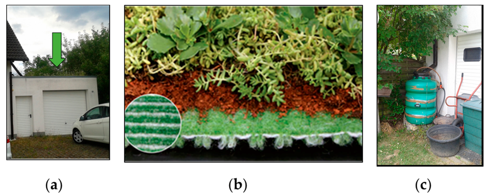
The case study is an extensive green roof with an area of 22 m2, a slope of about 5°, and a total depth of 20 cm. It is located on the garage of a one-family house in Bernkastel-Kues (49°55′11″ N, 7°4′33″ E, 145 m above sea level), Rhineland-Palatinate, the western part of Germany (Figure 1a). The roof is made up of three layers: the vegetation layer (spontaneous vegetation), the growing medium (mineral substrate), and a water storage/protective layer (retention Hydrotex membrane) (Figure 1b). The Hydrotex membrane has a thickness of 1 cm, a weight of 850 g/m2, and a horizontal permeability higher than 2.3 L/m∙s.
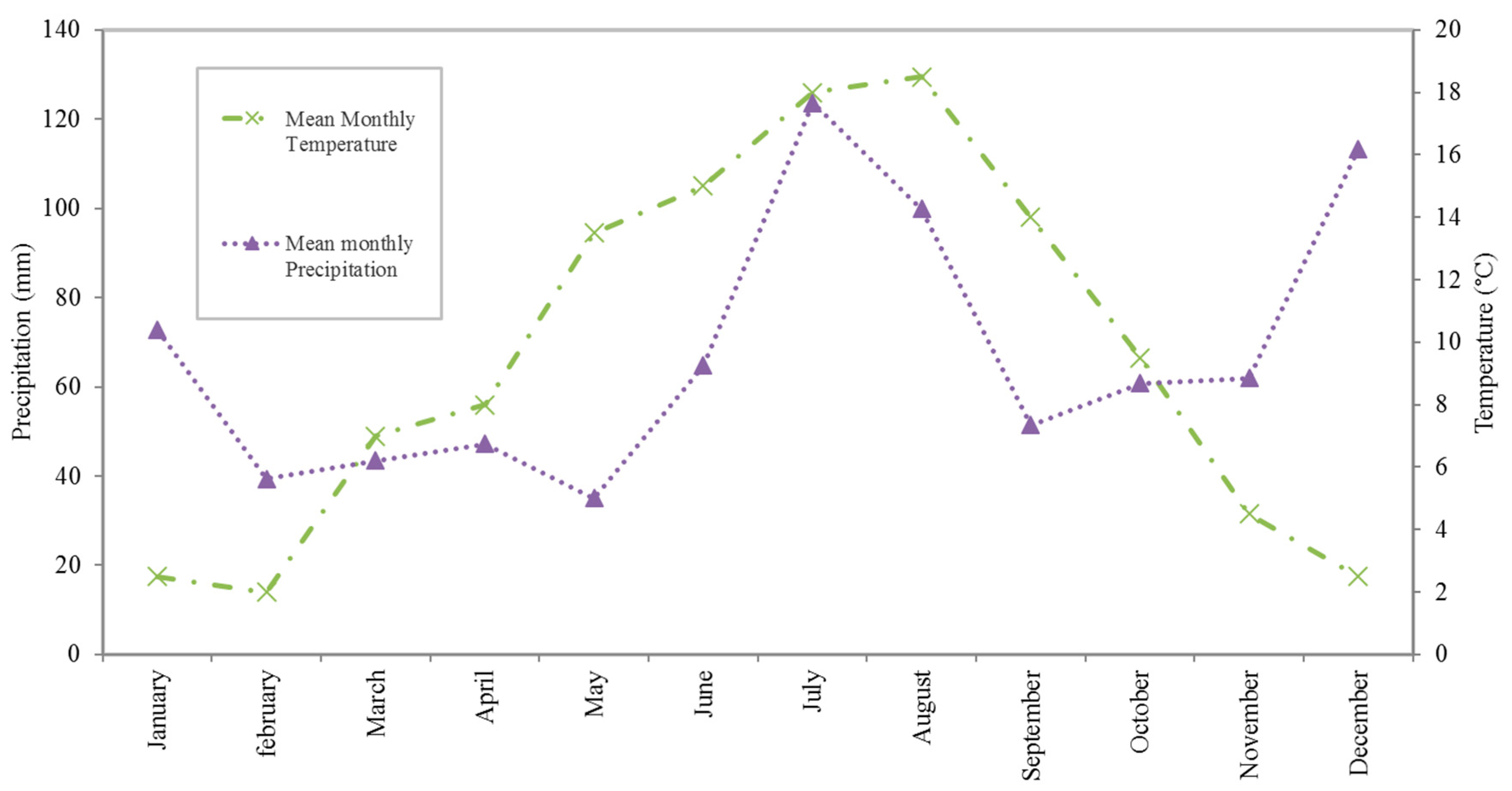
The runoff from the roof is channeled into a 500 L tank (Figure 1c) where the flow measurement has been performed by reading the actual water level in the reservoir daily. The climate regime is typically oceanic. The average precipitation is about 700–800 mm/year and it is approximately uniformly distributed during the year. Temperature exhibits instead a typical seasonal pattern, with the highest monthly mean values during the summer season of about 18 °C and annual average temperature of 9.4° (Figure 2). The meteorological data used in this work are precipitation recorded at the experimental site and wind speed, air temperature, relative humidity, global radiation collected at the nearest available meteorological station, Bernkastel (AgrarMeteorologie, Rheinland-Pfalz, www.am.rlp.de).
Runoff measurements have been recorded, with a daily time step, from March 2004 to May 2007, but some missing data appear during the monitoring period, preventing the total period of observation to be used for modeling purposes. Generally, no significant runoff has occurred, due to freezing of the water, between late December and late March. For this reason, the winter period has not been considered in the simulation approach.
2.2. Methodology
The aim of the reported research is an analysis of the impact of the complexity in the description of variables and processes of a green roof hydrological model on the relative parametrization and accuracy, with a focus on the retention capacity of the green infrastructure. To this purpose, a daily scale conceptual hydrological model is applied, based on water balance equations whose main input variables are the precipitation, the evapotranspiration loss, and the maximum water storage capacity, here called the storage threshold [20]. The model is used with three different settings (mod A, mod B, and mod C), characterized by increasing complexity in the description of the involved variables and processes (Table 1).
The three settings correspond to a basic approach based on the use of potential evapotranspiration and a constant storage threshold (mod A); an intermediate approach where actual evapotranspiration and a constant storage threshold are accounted (mod B); a detailed approach where actual evapotranspiration and a variable maximum water holding depth are used (mod C). The three conceptual retention models, of different complexity, are calibrated using the values of runoff recorded at the presented experimental site.
2.2.1. The Governing Equations
The water balance equations used to simulate the runoff production “R”, common to all of the three model settings, are [20]
where “t” is the daily time index, “V” the green roof water depth, “P” the observed precipitation, “ET” the modeled evapotranspiration loss, “Wmax” the maximum water-holding depth or storage threshold.
In the basic approach, ET loss is assumed to be set on the potential evapotranspiration (PET) and a constant storage threshold is also considered. The governing equations become
where the term “” is replaced by “”. As PET is rapidly computed form meteorological observation, Wmax represents the only model parameter to be calibrated.
Potential evapotranspiration represents an ideal process but for a better model performance, the actual evapotranspiration process should be modeled. Actual evapotranspiration AET modeling generally requires soil moisture, and soil and vegetation properties data. In the following, to keep to a minimum the number of needed information, an approach simply based on meteorological variables is used. The proposed model is based on the concept of the non-potential Priestley–Taylor model [21]. In the intermediate approach, ET loss is then assumed to be set on the non-potential Priestley–Taylor evapotranspiration (AET) and a constant storage threshold is accounted for. The governing equations are represented by Equation (3) where the term “” is replaced by “”:
As in the case of the basic model, in mod B of Table 1 Wmax represents the only parameter to be calibrated for hydrological simulation. Considered as the amount of water stored between the permanent wilting point and the field capacity, the maximum water holding capacity Wmax depends on substrate layer material properties and represents a constant physical threshold. The constant physical limit could be however called into the discussion, if it is considered that due soil heterogeneity runoff can occur even before the actual capacity is reached and that vegetation provides some additional moisture storage capacity to be accounted for [13]. Wmax is more likely to represent a process rather than a physical property and, as exhaustively discussed in [20], a strong correlation is found between the water holding capacity Wmax and the stored depth V, in that it can be assumed that
According to such discussion, in the mod C of Table 1, ET loss is assumed to be set on the actual evapotranspiration (AET) and a variable storage threshold is accounted for “” and “,” respectively, replace “” and “” in Equation (1) and the water balance equations are
where the second equation, according to Equation (4), can be rewritten as
Model details are more complex, as more processes are schematized, but contrary to what was expected, model parametrization is lessened, as no parameter has to be calibrated for simulation purposes.
2.2.2. Models Selection for Potential and Actual Evapotranspiration Assessment
Within the study area, there are no instruments to directly measure ET fluxes such as eddy covariance stations, chambers, sap flow systems, and weighing lysimeters. Due to the lack of observational flux data, a weighted and careful selection of the most accurate methods for the indirect ET modeling has not been possible and Penman formulation [22] has been considered for PET modeling while the API model [23] has been used to reproduce AET. According to the literature, the Penman model is one of the most commonly used methods for the assessment of PET in in-the-field research [24] so it has been chosen as it represents a well-consolidated approach. With regards to the API approach, even if less recent, this model has proven to perform well in similar studies where it has been compared with other ET methods including the AA (advection aridity) model [20,25].
The Penman Equation [22] can be expressed as
where λ (MJ kg−1) is the latent heat of vaporization:
T is the air temperature (°C), Rn (MJ m−2 day−1) is the net radiation, Gsoil (MJ m−2 day−1) is the soil heat flux considered to be negligible on a daily time scale [26], Δ (kPa °C−1) is the slope of the saturation vapor pressure-temperature relationship:
es is the saturation vapor pressure:
γ is the psychrometric constant (kPa °C−1), and EA is the drying power of the air expressed as
u is the wind speed (ms−1), ea is the vapor pressure (kPa).
Indirect estimation for actual evapotranspiration modeling is here proposed through the case of empirical relation that, opposite to more physically based methods, are simply based on routinely measured meteorological variables. Among these, methods with a firm physical analysis have been applied, in the past, based on the non-potential evapotranspiration concept by Priestley and Taylor [21,27,28]. The API (Antecedent Precipitation Index) approach models actual evapotranspiration modifying the potential evapotranspiration suggested by Priestley–Taylor with a coefficient α depending on the API [23] and representing the soil moisture content:
where α (-) is:
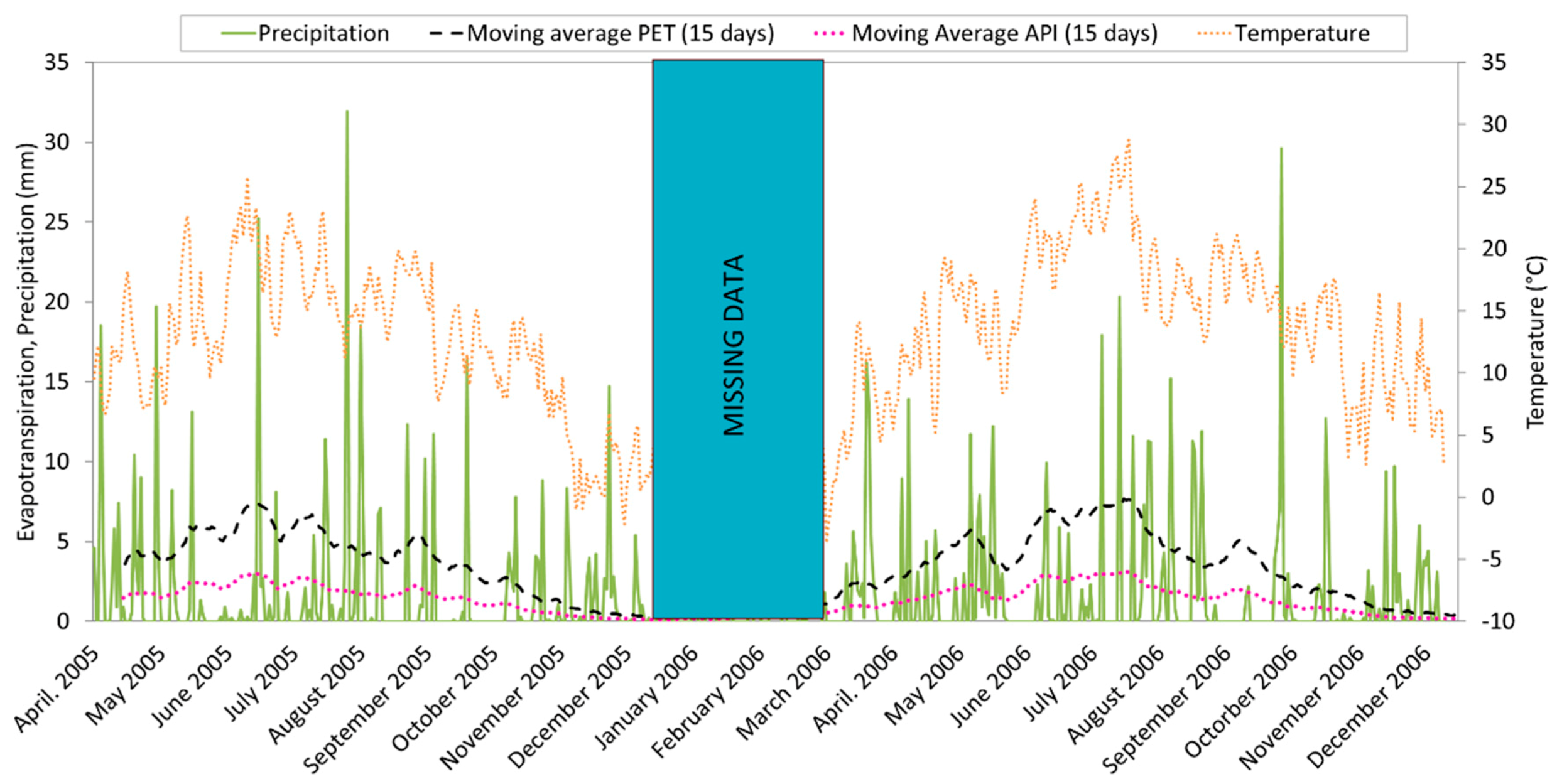
In Figure 3, the monthly patterns of potential, actual evapotranspiration, temperature and precipitation from April 2005 to December 2006 are shown. Potential fluxes approach actual during the cold and wet period from November to December.
3. Results
In the case of mod A and mod B settings, evapotranspiration losses, respectively potential and actual fluxes, represent functions of meteorological variables. They can be assessed a priori and used as a climate forcing for the GR model, not dependent on the stored water depth V. Mod A and mod B hydrological simulations rely thus only on Wmax calibration. In the case of mod C, as previously discussed Wmax is assumed to change during the simulation. This circumstance, as discussed, causes a simplification of the water balance equation, and the hydrological simulation does not require a calibration phase, with runoff production modeled as in Equation (6).
3.1. Models Evaluation
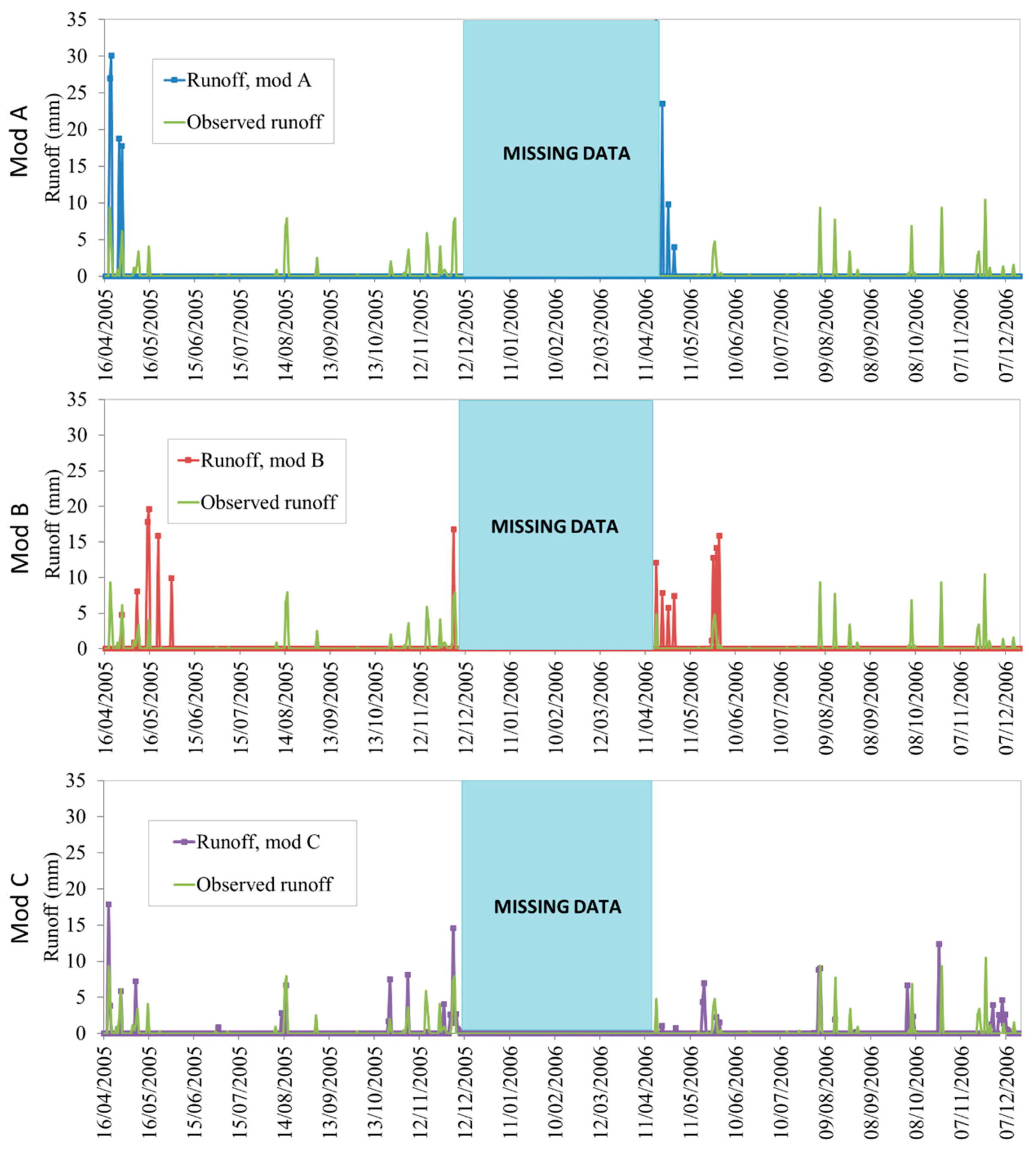
In the case of mod A and mod B, Wmax calibration is achieved assuming that total modeled runoff equals total observed runoff, for each period of simulation. This assumption, even though it appears simplified, allows us to streamline the calibration process and to reduce the computational efforts required by the models. In addition, because of missing observational data due to the temporary failure of the monitoring system, the event scale calibration is difficult to achieve. Such a calibration of the models allows one to obtain an accurate assessment of the long-term hydrological performances of the green roof at the cost of a less effective prediction of the runoff at finer scales. Results are illustrated in Figure 4 and Figure 5. At first visual inspection, in the case of mod A and mod B, several runoff events are not modeled and in most cases, an overestimation occurs. Mod C appears the best performing among the three different considered model settings. To quantitatively judge the ability of the approaches to reproduce the observed runoff, two fit indices, an average of absolute percentage errors (AAPE), root-mean-square errors (RMSE), and the percentage RMSE have been calculated:
with “n” the number of points of discontinuity of the cumulated runoff distribution (e.g., runoff events occurrences in Figure 5) where the fit is evaluated, Rmod is the modeled runoff, Robs the observed runoff, and the total average observed runoff. The results are illustrated in Table 2.
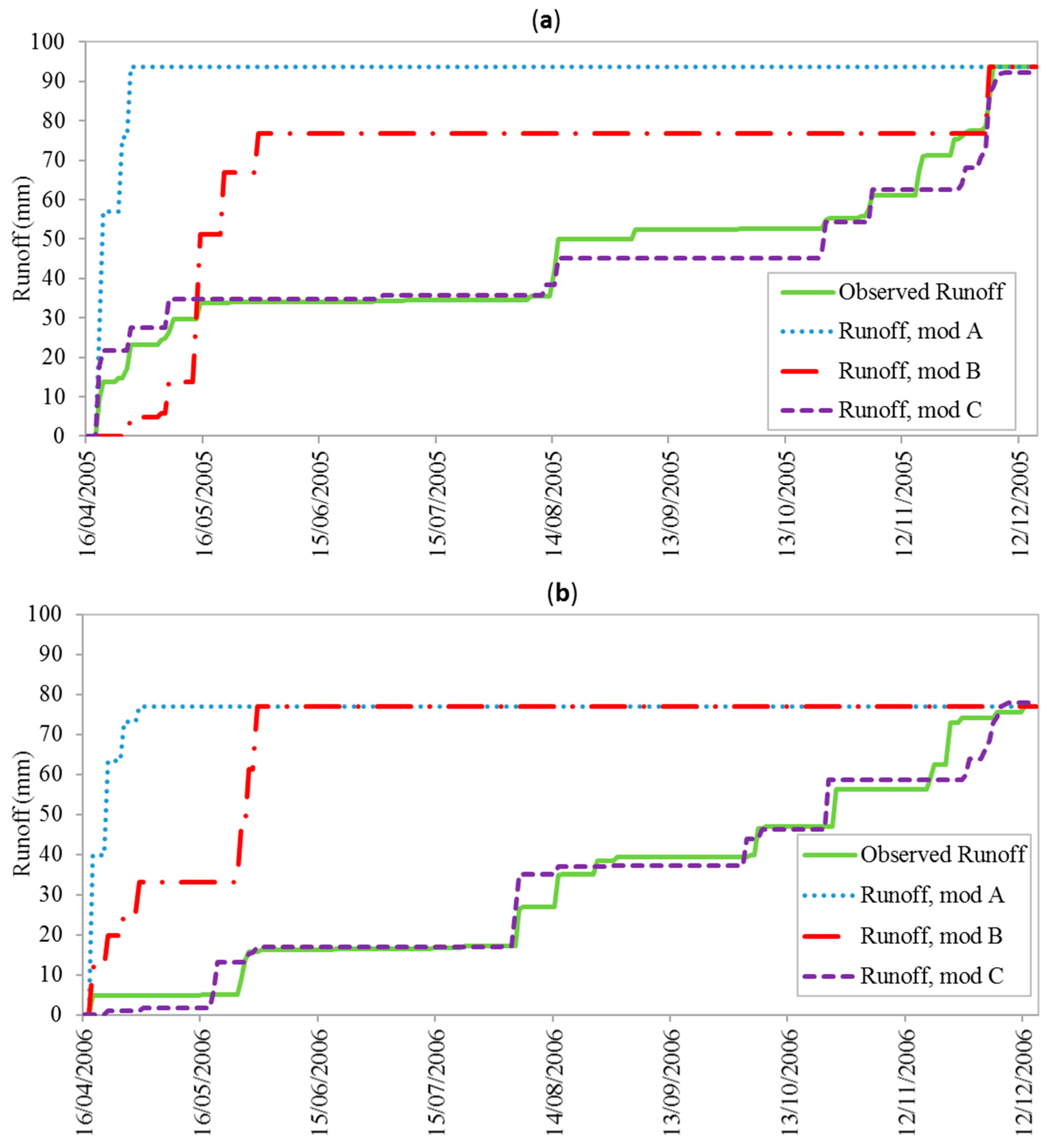
Although a calibration process has been performed and cumulative simulated runoff equals the observed one, mod A, regardless for the modeled period, is characterized by the largest errors, with RMSE (%) above 14% (in 2005), of average observed runoff, and AAPE approaching 126% (in 2005). Cumulative modeled runoff pattern significantly differs from the observed one and it is practically not at all affected from rainfall occurrences, as the cumulative runoff, for the total period of observation, is approached in the earlier period of the simulation (Figure 5). Moving from potential to actual evapotranspiration losses increases model accuracy. RMSE (%) and AAPE values for mod B are indeed lower than in the case of mod A, respectively equal to about 11% and 89% (in 2006), but cumulative simulated runoff pattern is still significantly different from the observed one. A larger sensitivity to rainfall occurrences is detected however compared to mod A (Figure 5). Despite the lack of a calibration process, mod C appears to be the best performing method also from a quantitative point of view. RMSE (%) and AAPE indices approach the lowest values of about 2% and 15% (for both years) respectively. Furthermore, a cumulated modeled pattern is very close to the observed one and total cumulated runoff only differs from about 1% from observed one (Figure 5). Calibrated values for the maximum water holding capacities for mod A and mod B are illustrated in Table 3 as a percentage of total soil depth.
The values assumed by the calibrated Wmax for both models and years can be discussed with reference to the cumulative evapotranspiration losses for each model and for each year. According to Equation (1), Wmax, which in the presented study does not represent a physical property, is called to balance the evapotranspiration losses in the hydrological model. Provided an observed amount of precipitation P and provided the calibration rule that is the cumulate observed runoff equal to the cumulated modeled runoff, larger ET losses are to be balanced by lower Wmax values. Comparing the Wmax values (for both years) for mod A and mod B, it can be observed that they are larger in the case of mod B, being the ET losses in the mod B schematized as the AET, lower than the PET accounted in mod A. The same justification can be provided for the difference in the Wmax values that for both models can be observed between the year 2005 and 2006. In the year 2006, the PET losses have been only 1% larger than PET losses in 2005. The difference in AET between the two years has been instead of about 6%. Wmax are then lower in 2006 compared to 2005 values to balance the larger ET losses in 2006 compared with the 2005 ET losses. Differences between 2005 and 2006 Wmax are negligible in the case of mod A (about 8%) which considers PET and very moderate in the case of mod B (about 15%) which considers the AET.
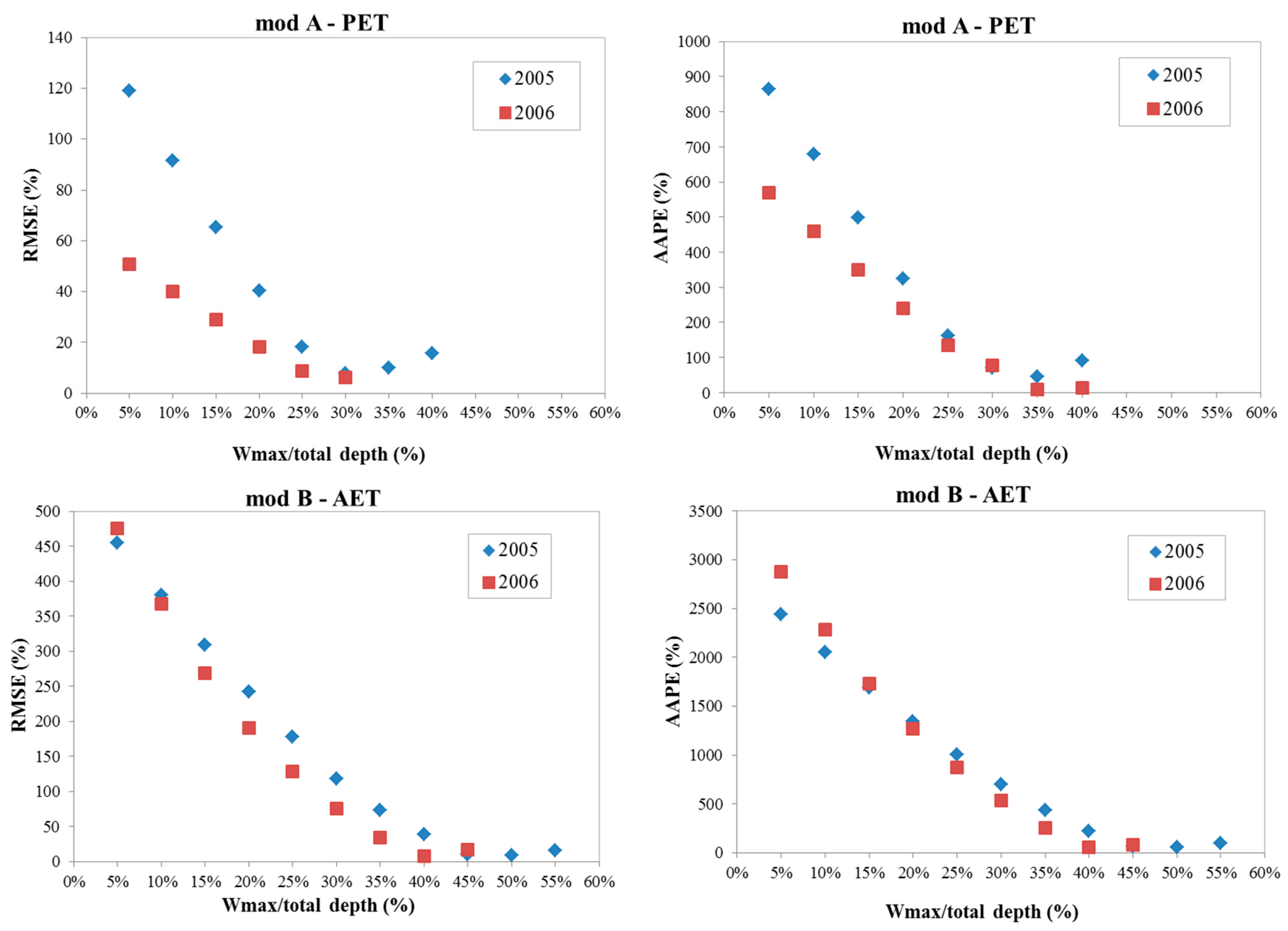
3.2. Impact of Maximum Water Holding Capacity Threshold
In the case of mod A and mod B the hydrological simulations require calibration for the water holding capacity threshold Wmax. For such approaches it would be important, especially in the context where experimental data are not available for calibration, to study the impact of the choice for a particular value of Wmax on model accuracy. To this purpose, a sensitivity analysis has been performed, in the case of mod A and mod B, to measure model performances through RMSE and AAPE statistical indices. The results are illustrated in Figure 6. For both cases, RMSE and AAPE illustrate how, as a result of the calibration, errors monotonically increase for Wmax values lower than the calibrated threshold. In the case of mod A, for a given Wmax value, errors occurring in 2005 and 2006 are different probably because the different cumulated runoff rates (Table 2) for the two periods are not balanced by instead very similar potential evapotranspiration cumulate loss for the same time intervals. The largest errors are indeed predicted for the 2005 period, characterized by the largest potential evapotranspiration loss. On the contrary, in the case of mod B, errors occurring in 2005 and 2006 are almost similar, probably because the different cumulated runoff rates (Table 2) for the two periods are balanced by a different actual evapotranspiration cumulate loss for the same time intervals. Model errors associated with mod B are compared to mod A, larger, for Wmax different from the calibrated threshold. Such circumstance indicates a larger sensitivity of mod B to uncalibrated Wmax compared to what occurs for mod A. Lower evapotranspiration losses (by an actual process as formulated in mod B) correspond to lower rainwater storage availability and thus, for a given Wmax, to larger runoff rates and larger overestimation (Figure 4).
4. Discussion and Conclusions
The present paper has presented a comparison of model performances, accuracies, and parametrization for three different hydrological green roof conceptual models aimed at the assessment of the green roof retention capacity. As a common feature, only meteorological data are needed for hydrological simulation for all of the proposed approaches. The three proposed models differ for the complexity of details in the formulation and schematization of the considered hydrological processes, from a basic (mod A) to an intermediate (mod B) to a more detailed approach (mod C). Mod A needs a little computational effort and technical expertise. It implements the potential evapotranspiration concept and it requires only basic meteorological input data which can be readily derived by publicly available databases. In mod A, a calibration process is performed through the comparison between the total modeled and measured runoff during the period of observation. Similar to the previous model, mod B carries out a calibration procedure of the storage threshold which is assumed constant but, on the other side, it requires the calculation of the actual evapotranspiration rates. Mod C sets ET on AET and considers a variable threshold as it represents a process rather than a physical property. So, this model embeds more detailed processes into hydrological modeling. Mod A is a basic approach and consequently, it is not able to predict the runoff production at event scale but is sufficient if the model user is interested in long term analysis of green roof potential runoff reduction and it can predict the total amount of runoff, in the long term, with a good degree of accuracy and with a relatively important sensitivity to model parameter calibration. The transition from mod A to mod B implies the increase in the prediction accuracy, but despite this, the model is mainly recommended for long term analysis of GR response. If interested in reproducing the behavior of the green system at a finer scale, model C can be used. Indeed, a more detailed model description has the benefit of improved model accuracy, as shown by the comparison of the computed statistical indices. This latter model can effectively simulate both the long-term green roof behavior and the daily scale GR performance. The correct assessment of both long term and single event GR hydrological response is crucial to identify the benefits of this green infrastructure in urban areas. Knowing the hydrological behavior at a finer scale allows one to quantify the rainfall attenuation during individual storms to face flooding events occurring in urban areas and to achieve sustainable urban drainage management. However, the long-term assessment of green roof hydrological performances is likewise essential. It provides an effective tool for practitioners, regulators, and engineers to make more informed decisions about GR implementation within urban areas. The economic benefits, at the hydrological level, of installing green roofs cannot be detectable immediately but in the long term indeed. A cost-benefit analysis, which is fundamental to justify the economic costs associated with green roofs, including the cost of installation and maintenance over time, would undoubtedly benefit from additionally account for the environmental benefits.
The findings of the present work are supported by several studies present in the scientific literature. Indeed, over time, many authors [19,29] compared hydrological models with different complexity to identify the best performing one for the assessment of GR hydrological performances. In [19], the accuracy of Storm Water management model (SWMM), Hydrus and Nash models in predicting the response of green roof to rainfall events have been compared. In terms of required input parameters and hydrological processes simulated in the model, the Nash approach results in the less complex method followed by Hydrus and SWMM. The RMSE decreases when switching from the less detailed model to the most detailed one. In particular, the Nash model is featured by an RMSE of 0.36 mm, Hydrus presents an error value of about 0.29 mm and SWMM returns an RMSE of about 0.28 mm. Similar results come out from [29], where a comparative study which refers to rainfall-runoff modeling, between SWMM and Fuzzy Logic Approach has been proposed. The fuzzy logic model outperforms the SWMM returning lower errors. In detail, RMSE is 3.31 mm for SWMM and 2.44 mm for the Fuzzy Logic Model. In [30] a comparison, in terms of Nash–Sutcliffe efficiency index (NSE), between a linear reservoir model and Hydrus has been set up with the result that the mechanistic model, which uses more details in the description of hydrological processes, returns higher performances than the conceptual approach. The average NSE is 0.87 for Hydrus and 0.70 for the reservoir model. Other authors [31] compared complex approaches able to model Low Impact Development (LID) practices incorporated within the drainage network with the finite element model with the results that generally the first outperforms the second ones. In this case, the first kind of model exhibits a value of NSE of 0.88 against 0.79 of the finite element model for events with rainfall intensity of 1.5 mm/min and 0.81 mm against 0.76 for storms with the intensity of 2 mm/min. These researches confirm what demonstrated in the current work namely that, the model accuracy increases with the details in model description, indeed, moving from the mod A to mod B to mod C, the errors assume the values of 13.15, 5.83, and 1.75 mm for 2005 and 146.30, 89.87, and 15.64 mm for 2006.
Author Contributions
Conceptualization, A.L.; Methodology, A.L.; Validation, M.M.; Formal analysis, M.M.; investigation, A.L. and M.M.; Data curation, M.M.; Writing—original draft preparation, A.L. and M.M.; Writing—review and editing, A.L. and M.M.; Supervision, A.L. All authors have read and agreed to the published version of the manuscript.
Funding
This research received no external funding.
Acknowledgments
Authors express their sincere gratitude to Joachim Sartor (Trier University of Applied Sciences) for providing runoff data from the experimental green roof and for his helpful suggestions and guidance during the research.
Conflicts of Interest
The authors declare no conflict of interest.
References
- Cettner, A.; Ashley, R.; Hedström, A.; Viklander, M. Sustainable development and urban stormwater practice. Urban Water J. 2013, 11, 185–197. [Google Scholar] [CrossRef]
- Shaharuddin, A.; Noorazuan, M.H.; Yaakob, M.J. Green roofs as best management practices for heat reduction and stormwater flow mitigation. World Appl. Sci. J. 2011, 13, 58–62. [Google Scholar]
- Sartor, J.; Mobilia, M.; Longobardi, A. Results and findings from 15 years of sustainable urban storm water management. Int. J. Saf. Secur. Eng. 2018, 8, 505–514. [Google Scholar] [CrossRef]
- Mobilia, M.; Longobardi, A. Smart stormwater management in urban areas by roofs greening. Lect. Notes Comput. Sci. 2017, 10406, 455–463. [Google Scholar] [CrossRef]
- Versini, P.-A.; Jouve, P.; Ramier, D.; Berthier, E.; De Gouvello, B. Use of green roofs to solve storm water issues at the basin scale—Study in the Hauts-de-Seine County (France). Urban Water J. 2015, 13, 372–381. [Google Scholar] [CrossRef] [Green Version]
- Krasnogorskaya, N.; Longobardi, A.; Mobilia, M.; Khasanova, L.F.; Shchelchkova, A.I. Hydrological modeling of green roofs runoff by Nash cascade model. Open Civ. Eng. J. 2019, 13, 163–171. [Google Scholar] [CrossRef]
- Gibler, M.R. Comprehensive benefits of green roofs. In Proceedings of the World Environmental and Water Resources Congress 2015: Floods, Droughts, and Ecosystems, Austin, TX, USA, 17–21 May 2015; pp. 2244–2251. [Google Scholar]
- Stovin, V.; Vesuviano, G.; De-Ville, S. Defining green roof detention performance. Urban Water J. 2015, 14, 1–15. [Google Scholar] [CrossRef] [Green Version]
- Mentens, J.; Raes, D.; Hermy, M. Green roofs as a tool for solving the rainwater runoff problem in the urbanized 21st century? Landsc. Urban Plan. 2006, 77, 217–226. [Google Scholar] [CrossRef]
- Teemusk, A.; Mander, Ü. Rainwater runoff quantity and quality performance from a greenroof: The effects of short-term events. Ecol. Eng. 2007, 30, 271–277. [Google Scholar] [CrossRef]
- Longobardi, A.; D’Ambrosio, R.; Mobilia, M. Predicting stormwater retention capacity of green roofs: An experimental study of the roles of climate, substrate soil moisture, and drainage layer properties. Sustainability 2019, 11, 6956. [Google Scholar] [CrossRef] [Green Version]
- Stovin, V.; Vesuviano, G.; Kasmin, H. The hydrological performance of a green roof test bed under UK climatic conditions. J. Hydrol. 2012, 414, 148–161. [Google Scholar] [CrossRef]
- Poë, S.; Stovin, V.; Berretta, C. Parameters influencing the regeneration of a green roof’s retention capacity via evapotranspiration. J. Hydrol. 2015, 523, 356–367. [Google Scholar] [CrossRef]
- Starry, O.; Lea-Cox, J.; Ristvey, A.; Cohan, S. Parameterizing a water-balance model for predicting stormwater runoff from green roofs. J. Hydrol. Eng. 2016, 21, 04016046. [Google Scholar] [CrossRef] [Green Version]
- Feitosa, R.C.; Wilkinson, S.J. Modelling green roof stormwater response for different soil depths. Landsc. Urban Plan. 2016, 153, 170–179. [Google Scholar] [CrossRef]
- Voyde, E.; Fassman, E.; Simcock, R.; Wells, J.; Fassman-Beck, E. Quantifying evapotranspiration rates for new zealand green roofs. J. Hydrol. Eng. 2010, 15, 395–403. [Google Scholar] [CrossRef]
- Burszta-Adamiak, E.; Mrowiec, M. Modelling of green roofs’ hydrologic performance using EPA’s SWMM. Water Sci. Technol. 2013, 68, 36–42. [Google Scholar] [CrossRef]
- Carson, T.; Keeley, M.; Marasco, D.E.; McGillis, W.; Culligan, P. Assessing methods for predicting green roof rainfall capture: A comparison between full-scale observations and four hydrologic models. Urban Water J. 2015, 14, 589–603. [Google Scholar] [CrossRef]
- Mobilia, M.; Longobardi, A. Impact of rainfall properties on the performance of hydrological models for green roofs simulation. Water Sci. Technol. 2020. [Google Scholar] [CrossRef]
- Mobilia, M.; Longobardi, A.; Sartor, J.F. Including a-priori assessment of actual evapotranspiration for green roof daily scale hydrological modelling. Water 2017, 9, 72. [Google Scholar] [CrossRef] [Green Version]
- Mawdsley, J.A.; Ali, M.F. Estimating nonpotential evapotranspiration by means of the equilibrium evaporation concept. Water Resour. Res. 1985, 21, 383–391. [Google Scholar] [CrossRef]
- Penman, H.L. Natural evaporation from open water, bare soil and grass, proceedings of the royal society of London. Ser. Math. Phys. Eng. Sci. 1948, 193, 120–145. [Google Scholar]
- Linsley, R.K.; Kohler, M.A. Variations in storm rainfall over small areas. Trans. Am. Geophys. Union 1951, 32, 245. [Google Scholar] [CrossRef]
- Bogawski, P.; Bednorz, E. Comparison and validation of selected evapotranspiration models for conditions in Poland (Central Europe). Water Resour. Manag. 2014, 28, 5021–5038. [Google Scholar] [CrossRef] [Green Version]
- Marasco, D.E.; Culligan, P.J.; McGillis, W.R. Evaluation of common evapotranspiration models based on measurements from two extensive green roofs in New York City. Ecol. Eng. 2015, 84, 451–462. [Google Scholar] [CrossRef] [Green Version]
- Purdy, A.J.; Fisher, J.B.; Goulden, M.L.; Famiglietti, J. Ground heat flux: An analytical review of 6 models evaluated at 88 sites and globally. J. Geophys. Res. Biogeosci. 2016, 121, 3045–3059. [Google Scholar] [CrossRef]
- Priestley, C.H.B.; Taylor, R.J. On the assessment of surface heat flux and evaporation using large-scale parameters. Mon. Weather Rev. 1972, 100, 81–92. [Google Scholar] [CrossRef]
- Davies, J.A.; Allen, C.D. Equilibrium, potential and actual evaporation from cropped surfaces in Southern Ontario. J. Appl. Meteorol. 1973, 12, 649–657. [Google Scholar] [CrossRef] [Green Version]
- Wang, K.-H.; Altunkaynak, A. Comparative case study of rainfall-runoff modeling between SWMM and fuzzy logic approach. J. Hydrol. Eng. 2012, 17, 283–291. [Google Scholar] [CrossRef]
- Palla, A.; Gnecco, I.; Lanza, L.G. Compared performance of a conceptual and a mechanistic hydrologic models of a green roof. Hydrol. Process. 2011, 26, 73–84. [Google Scholar] [CrossRef]
- Haowen, X.; Yawen, W.; Luping, W.; Weilin, L.; Wenqi, Z.; Hong, Z.; Yichen, Y.; Jun, L. Comparing simulations of green roof hydrological processes by SWMM and HYDRUS-1D. Water Supply 2019, 20, 130–139. [Google Scholar] [CrossRef]
Figure 1.
(a) Green roof location; (b) cross-section of the green roof; (c): Runoff collection tank.
Figure 1.
(a) Green roof location; (b) cross-section of the green roof; (c): Runoff collection tank.

Figure 2.
Patterns of long-term mean monthly rain and temperature for the study site.

Figure 3.
Daily patterns of potential evapotranspiration (PET), actual evapotranspiration (AET), temperature and precipitation during the period of observation.
Figure 3.
Daily patterns of potential evapotranspiration (PET), actual evapotranspiration (AET), temperature and precipitation during the period of observation.

Figure 4.
Comparison between modeled and observed runoff time series for the different approaches.

Figure 5.
Comparison between cumulated observed runoff from the studied green roof and cumulated runoff modeled using the three approaches with increasing level of complexity. (a) simulated period: 2005. (b) simulated period: 2006.
Figure 5.
Comparison between cumulated observed runoff from the studied green roof and cumulated runoff modeled using the three approaches with increasing level of complexity. (a) simulated period: 2005. (b) simulated period: 2006.

Figure 6.
Impact of water holding capacity (as a percentage of soil total depth) for mod A (upper panel) and mod B (lower panel) on RMSE and AAPE values.
Figure 6.
Impact of water holding capacity (as a percentage of soil total depth) for mod A (upper panel) and mod B (lower panel) on RMSE and AAPE values.


Table 1.
Models settings for different model complexity level. Mod A represents the basic approach. Mod B represents the intermediate approach. Mod C represents the detailed approach. (ET: Evapotranspiration, PET: Potential Evapotranspiration, AET: Actual evapotranspiration, Wmax: Maximum water holding capacity)
| Method | ET | Wmax |
|---|---|---|
| mod A | PET | Constant |
| mod B | AET | Constant |
| mod C | AET | Variable |
Table 2.
Values of the root-mean-square errors (RMSE) and absolute percentage errors (AAPE) for the different approaches.
Table 2.
Values of the root-mean-square errors (RMSE) and absolute percentage errors (AAPE) for the different approaches.
| Year | Method | Rmod (mm) | RMSE (mm) | AAPE (%) |
|---|---|---|---|---|
| 2005 Robs(mm) = 93.6 | mod A | 93.64 | 13.15 | 126.40 |
| mod B | 93.64 | 5.83 | 48.17 | |
| mod C | 92.34 | 1.75 | 13.08 | |
| 2006 Robs(mm) = 77.0 | mod A | 77.05 | 146.50 | 9.79 |
| mod B | 77.05 | 89.87 | 8.71 | |
| mod C | 77.91 | 15.64 | 1.53 |
Table 3.
Calibrated (mod A and mod B) maximum water holding capacities as a percentage of total soil depth.
Table 3.
Calibrated (mod A and mod B) maximum water holding capacities as a percentage of total soil depth.
| Year | Mod A (%) | Mod B (%) |
|---|---|---|
| 2005 | 26.6 | 46.1 |
| 2006 | 24.3 | 38.9 |
© 2020 by the authors. Licensee MDPI, Basel, Switzerland. This article is an open access article distributed under the terms and conditions of the Creative Commons Attribution (CC BY) license (http://creativecommons.org/licenses/by/4.0/).
Share and Cite
MDPI and ACS Style
Mobilia, M.; Longobardi, A. Model Details, Parametrization, and Accuracy in Daily Scale Green Roof Hydrological Conceptual Simulation. Atmosphere 2020, 11, 575. https://doi.org/10.3390/atmos11060575
AMA Style
Mobilia M, Longobardi A. Model Details, Parametrization, and Accuracy in Daily Scale Green Roof Hydrological Conceptual Simulation. Atmosphere. 2020; 11(6):575. https://doi.org/10.3390/atmos11060575
Chicago/Turabian StyleMobilia, Mirka, and Antonia Longobardi. 2020. "Model Details, Parametrization, and Accuracy in Daily Scale Green Roof Hydrological Conceptual Simulation" Atmosphere 11, no. 6: 575. https://doi.org/10.3390/atmos11060575
Note that from the first issue of 2016, this journal uses article numbers instead of page numbers. See further details here.