Article

Improved Simulation of the Antarctic Stratospheric Final Warming by Modifying the Orographic Gravity Wave Parameterization in the Beijing Climate Center Atmospheric General Circulation Model

1
Beijing Climate Center, China Meteorological Administration, Beijing 100081, China
2
Key Laboratory of Mesoscale Severe Weather/Ministry of Education, School of Atmospheric Sciences, Nanjing University, Nanjing 210023, China
*
Author to whom correspondence should be addressed.
Atmosphere 2020, 11(6), 576; https://doi.org/10.3390/atmos11060576
Submission received: 27 April 2020 / Revised: 20 May 2020 / Accepted: 29 May 2020 / Published: 1 June 2020
(This article belongs to the Special Issue Gravity Waves in the Atmosphere)

Abstract

:
The Antarctic stratospheric final warming (SFW) is usually simulated with a substantial delay in climate models, and the corresponding temperatures in austral spring are lower than observations, implying insufficient stratospheric wave drag. To investigate the role of orographic gravity wave drag (GWD) in modeling the Antarctic SFW, in this study the orographic GWD parameterization scheme is modified in the middle-atmosphere version of the Beijing Climate Center Atmospheric General Circulation Model. A pair of simulations are conducted to compare two orographic GWD schemes in simulating the breakdown of the stratospheric polar vortex over Antarctica. The control simulation with the default orographic GWD scheme exhibits delayed vortex breakdown and the cold-pole bias seen in most climate models. In the simulation with modified orographic GWD scheme, the simulated vortex breaks down earlier by 8 days, and the associated cold-pole bias is reduced by more than 2 K. The modified scheme provides stronger orographic GWD in the lower stratosphere, which drives an accelerated polar downwelling branch of the Brewer–Dobson circulation and, in turn, produces adiabatic warming. Our study suggests that modifying orographic GWD parameterizations in climate models would be a valid way of improving the SFW simulation over Antarctica.

Graphical Abstract

1. Introduction

Climate models have evolved into the stage of “Earth System Models” (ESMs), in which various components of physics, chemistry, and biology are fully coupled to serve multiple purposes, including the simulation of air quality, stratospheric ozone, tropospheric chemistry, and global climate. As a major model hierarchy of ESMs, chemistry-climate models (CCMs) combine physical climate models with an explicit representation of atmospheric chemistry and have been used in investigating the Antarctic ozone depletion problem [1,2]. Despite significant improvements in modelling, the simulated Antarctic stratospheric vortex breaking down too late in the year is a common bias to in almost all CCMs. The breakdown of the Southern Hemisphere polar vortex, hereafter referred to as Antarctic stratospheric final warming (SFW), marks the transition of middle-atmospheric circulation from winter to summer. However, the Antarctic SFW simulated by a number of climate models is 1–2 weeks later than observations at 50 hPa [3,4,5]. As a result, the polar temperatures in climate models are often considerably colder than observed during austral winter and spring. This systematic cold-pole bias is a long existing problem, and it continues to remain a severe impediment to progress [6]. These temperature and wind biases have significant implications for the simulation of Antarctic ozone. They can result in a late seasonal ozone recovery and lead to simulated ozone trends in the Antarctic stratosphere, which are offset by several weeks against observations [7,8,9]. Furthermore, simulations that incorporate a chemistry scheme sensitive to temperature tend to produce unrealistically large ozone loss over Antarctica [10].
The root cause of the cold-pole bias is the deficiency of model dynamics [11,12]. The downwelling branch of the wave-driven Brewer–Dobson circulation (BDC), which produces adiabatic warming, largely determines the temperature in the polar stratosphere. The extratropical BDC is driven by both large-scale planetary waves and small-scale gravity waves (GWs). Both types of waves drive the BDC in different ways. The planetary waves primarily affect the BDC through Rossby-wave pumping, while GWs affect the BDC by modulating the adiabatic upwelling into the mesosphere [13,14,15]. The cold-pole bias in Antarctic winter and spring points to missing wave forcing of the BDC, which could be attributed to resolved planetary waves, GWs, or a combination of the two. In global climate models with moderate spatio-temporal resolution (~1°–2°), the drag exerted on the atmosphere by GWs is commonly parameterized as it is a subgrid-scale process. The fact that almost all CCMs suffer from a delayed breakdown of the stratospheric polar vortex in Antarctic spring implies that GWs are responsible for the insufficient drag, which is closely related to how GW parameterizations are constructed [16].
Parameterization schemes for GWs generated by flow over orography are often blamed for the polar stratospheric temperature and zonal wind biases in CCMs, which could be related to a deficit of orographic gravity wave drag (GWD) near 60° S. Numerical studies have indicated that the cold-pole bias is considerably reduced and the polar vortex breaks down earlier when an additional source of orographic GWs centered on 60° S is prescribed [11]. One possible source of missing orographic GWD is from small isolated mountainous islands in the Southern Ocean near 60° S, which can produce large momentum fluxes but are not properly resolved in the models because of their poor resolutions [17,18]. Another possible contributor to the absent orographic GWD around 60° S is the simplified assumption that the waves propagate straight up, which is adopted in nearly all current orographic GWs parameterizations. However, simulation results from high-resolution models indicate that resolved small-scale GWs can horizontally propagate into the Southern Ocean from the Antarctic Peninsula and southern Andes [19,20]. Based on global positioning system data, observational studies also reveal that GW activity near 60° S laterally propagates from lower latitudes over the southern Andes [21]. The abovementioned cases of GW absence from both small islands and horizontal propagation, leading to an unphysical gap in the parameterized orographic GWD near 60° S, are common to all CCMs and thus potentially responsible for the delayed SFW over Antarctica.
Except for the missing orographic GWD near 60° S, the existing orographic GWD parameterization schemes currently used in climate models are constructed at different levels of complexity. The goal of the present study is to compare two orographic GWD schemes in modeling the Antarctic SFW in a middle-atmosphere version of the Beijing Climate Center Atmospheric Circulation Model (BCC-AGCM). The middle-atmosphere version of the BCC-AGCM includes traditional parameterizations of orographic GWs [22], as well as state-of-the-art parameterizations of nonorographic GWs tied to their tropospheric sources [23,24]. Given the planned development of the BCC-AGCM to a CCM, alleviating the stratospheric cold-pole bias which impacts the amount of Antarctic ozone depletion is essential. Both orographic and nonorographic GWD can play an important role in mitigating the cold-pole bias. Focusing on the Antarctic SFW, the purpose of this study is to demonstrate the influence of orographic GWD parameterizations on simulating the dynamics and temperature of the middle atmosphere. The remainder of this paper is organized as follows. Section 2 describes the middle-atmosphere version of BCC-AGCM and outlines the two orographic GW schemes. The experimental design and analysis methods are also presented in Section 2. In Section 3, the improved Antarctic SFW simulation and the changes in wave forcing resulting from modifying the orographic GWs schemes are illustrated. Section 4 summarizes our findings and discusses the uncertainties associated with modifying GW parameterizations to improve the dynamical performance of climate models.

2. Model, Experiments, and Analysis Methods

2.1. General Description of the Middle-Atmosphere Version of BCC-AGCM

In this study, the numerical simulations were carried out with the middle-atmosphere configuration of the medium-resolution Beijing Climate Center Atmospheric General Circulation Model version 3 (BCC-AGCM3-MR) [25]. The original BCC-AGCM3-MR, which participates in the Coupled Model Intercomparison Project Phase 6 (CMIP6), has a spectral truncation at wavenumber 106 with an associated Gaussian grid of 1.125° resolution. The CMIP6 configuration of the BCC-AGCM3-MR contains 46 hybrid vertical levels with approximately 800-m vertical spacing throughout the midtroposphere and lower stratosphere. The model top is at about 1.98 hPa and the vertical spacing of the top model layer is about 3.8 km. The CMIP6 version of the BCC-AGCM3-MR uses two distinct GWD parameterizations, which represent GWs generated by subgrid-scale orography [22], and by convection [23], respectively. The convective GW parameterization depends on the deep convective heating properties and the background wind, and benefits a spontaneous stratospheric quasi-biennial oscillation [26]. In the present study, the number of model layers has been increased to 95, with an elevated model top up to 0.01 hPa or approximately 80 km. The typical vertical resolution of the 95-layer grid is 700 m from the midtroposphere to the lower stratosphere and better than 1 km up to the stratopause. In addition to the processes represented in the original BCC-AGCM3-MR, the middle-atmosphere version also includes a GW parameterization for the momentum flux deposition from fronts and jet imbalances [24]. Both of the convective and front-jet GW parameterizations used in this high-top model are source-related and supposed to cover all the GWs of nonorographic origins. Furthermore, the middle-atmosphere configuration employs a parameterization to estimate the turbulent mountain stress caused by unresolved orography, which has been proved to be important in simulating the sudden stratospheric warming events in boreal winter by influencing the propagation of planetary waves into the polar vortex [27]. The upward extension of BCC-AGCM3-MR into the middle atmosphere documented here is in the absence of chemistry, and acts as a base model for future chemistry climate modeling efforts. The primary purpose of this middle-atmosphere model is to gain a climatology of winds and temperatures that is suitable for investigating climate issues related to ozone. One prominent problem is the breakdown timing of the Southern Hemisphere stratospheric polar vortex.

2.2. Parameterization of Orographic GWs

In the default BCC-AGCM3-MR and its middle-atmosphere configuration, the drag from dissipating GWs forced by flow over orography is parameterized as in McFarlane (1987) [22]. The McFarlane (1987) scheme is a conventional orographic GWD scheme, in which the wave amplitude is represented in terms of the standard deviation of the subgrid-scale orographic heights (σ). Waves are launched at the lowest model level and propagate vertically according to Lindzen’s wave saturation theory [28], which defines the saturation momentum flux as
τ * = ρ ¯ 0 k | U | 3 2 N
where ρ ¯ 0 , k, U, and N are the atmospheric density, the horizontal wave number, the background zonal wind, and the buoyancy frequency, respectively. When a wave becomes saturated and begins to break, the drag within a saturated region is determined from
U t = α 1 ρ ¯ 0 τ * z
where α is an efficiency factor which is tunable and is set to 0.125 in this study.
To investigate the impact of different orographic GW parameterizations on the simulated Antarctic SFWs, the orographic GWD scheme of Kim and Doyle (2005) [29] is implemented in the middle-atmosphere model used in this study. Compared with the McFarlane (1987) scheme, the Kim and Doyle (2005) scheme incorporates the effects of orographic asymmetry, convexity, and anisotropy, which are linked to the characteristics of the corresponding GWs. The orographic GWs in the Kim and Doyle (2005) scheme are emitted from the reference level, which is defined as the larger of the two values of 2σ and the boundary layer height. A model layer is considered unstable if the minimum Richardson number defined by
R i m = R i ( 1 F r d ) ( 1 + R i F r d ) 2
becomes less than its critical value Ric, where Ri is the Richardson number and F r d h d N / U . Here, hd is the vertical displacement height. Ric is a tunable parameter and is set to 0.25 in this study. Rim determines the onset of wave breaking. Wave breaking occurs when Rim < Ric (=0.25). It should be noted that the flow-blocking drag parameterization in the Kim and Doyle (2005) scheme is given by a separate formulation and not activated in this study, and is also absent in the McFarlane (1987) scheme.

2.3. Experimental Design

As shown in Table 1, two sets of 35-year Atmospheric Model Intercomparison Project (AMIP)-type simulations were conducted with the same prescribed sea surface boundary conditions using the Hadley Centre sea surface temperatures and sea ice concentrations from 1978 to 2012. The simulation using the default McFarlane (1987) [22] scheme is referred to as M87, and the other employing the Kim and Doyle (2005) [29] scheme is referred to as KD05. For each integration, the first year is treated as the spinup, and the last 34 years are used for analysis. Both runs start from identical initial conditions. Historical forcing data are based on observations and mainly include the monthly updated greenhouse gas concentrations with zonal mean values, the stratospheric aerosols from volcanoes, the time-varying gridded ozone concentrations, the anthropogenic aerosol optical properties, the solar forcing, and the yearly global gridded land use. It should be noted that only one 35-year run for each experiment is performed, which is not enough to take into account the internal atmospheric variability adequately as in the ensemble simulations. In order to evaluate the simulated Antarctic SFWs, wind velocities and temperatures from the Japanese Meteorological Agency 55-year Reanalysis (JRA-55) spanning from 1979 to 2012 are used as observational references [30].

2.4. The Transformed Eulerian-Mean (TEM) Framework

In this study, we examine the simulated BDC and forcing from resolved planetary waves in the framework of the TEM equations [31], which can be expressed as
u ¯ t = ( 1 a cos φ ( u ¯ cos φ ) φ f ) v ¯ * u ¯ z w ¯ * + 1 ρ 0 a cos φ F + X ¯
where u ¯ is the zonal mean zonal wind, φ is latitude, a is the radius of the earth, z is log-pressure height, f is the Coriolis parameter, ρ 0 is the density, the overbar represents zonal average, and subscripts represent the derivatives with respect to the given variable. The first and second terms on the right-hand side of Equation (4) denote acceleration associated with the residual mean meridional circulation ( v ¯ * , w ¯ * ) , i.e., the BDC:
v ¯ * = v ¯ 1 ρ 0 ( ρ 0 v θ ¯ θ ¯ z ) z
w ¯ * = w ¯ + 1 a cos φ ( cos φ v θ ¯ θ ¯ z ) φ
where v ¯ and w ¯ are the Eulerian mean meridional circulation, θ is potential temperature, and prime represents the departure from zonal mean. The third term on the right-hand side of Equation (4) is the divergence of the Eliassen–Palm (E-P) flux
F = 1 a cos φ ( F ( φ ) cos φ ) φ + F z ( z )
where
F ( φ ) = ρ 0 a cos φ ( v θ ¯ θ ¯ z u ¯ z v u ¯ )
F ( z ) = ρ 0 a cos φ [ ( f 1 a cos φ ( u ¯ cos φ ) φ ) v θ ¯ θ ¯ z w u ¯ ]
and F = ( F ( φ ) , F ( z ) ) is the E-P flux vector. The E-P flux divergence F measures the forcing from resolved waves. The forcing from other processes including GWD is represented by the X ¯ term.

3. Results

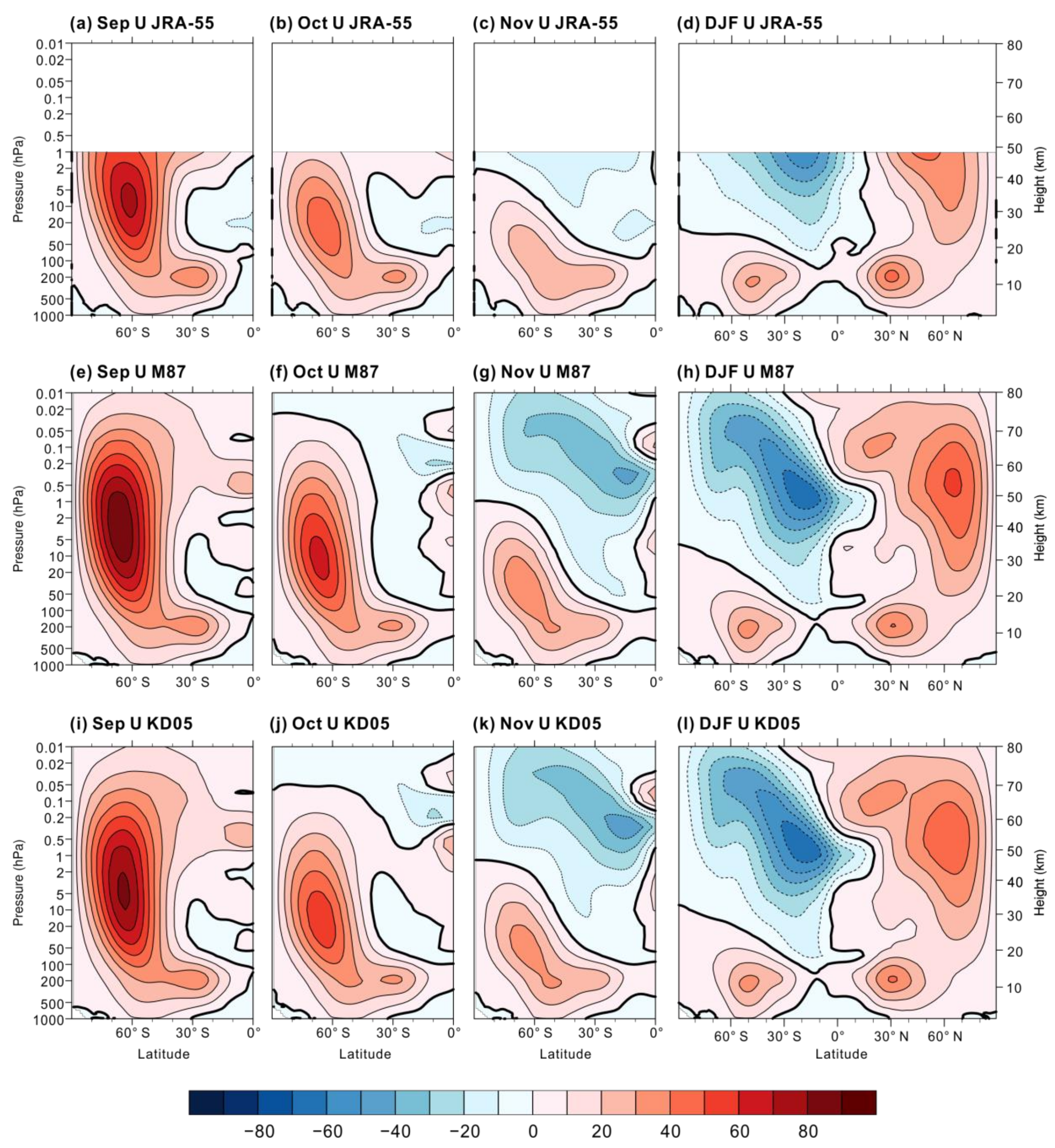
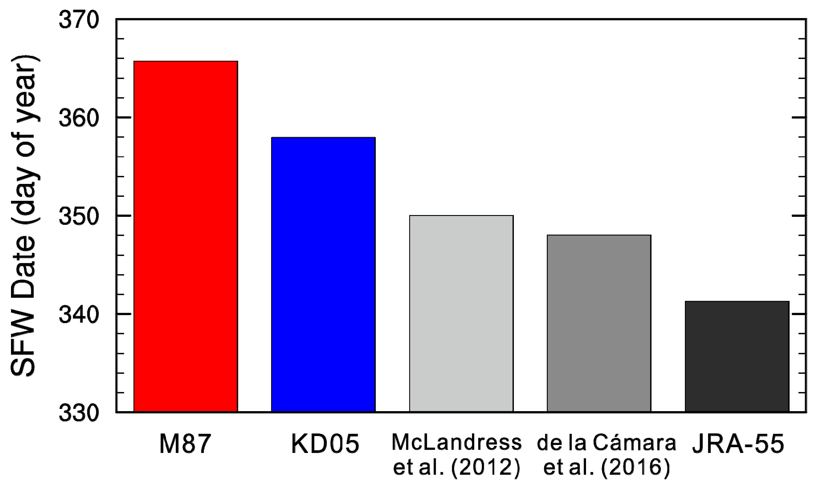
3.1. The Austral SFW in the BCC-AGCM
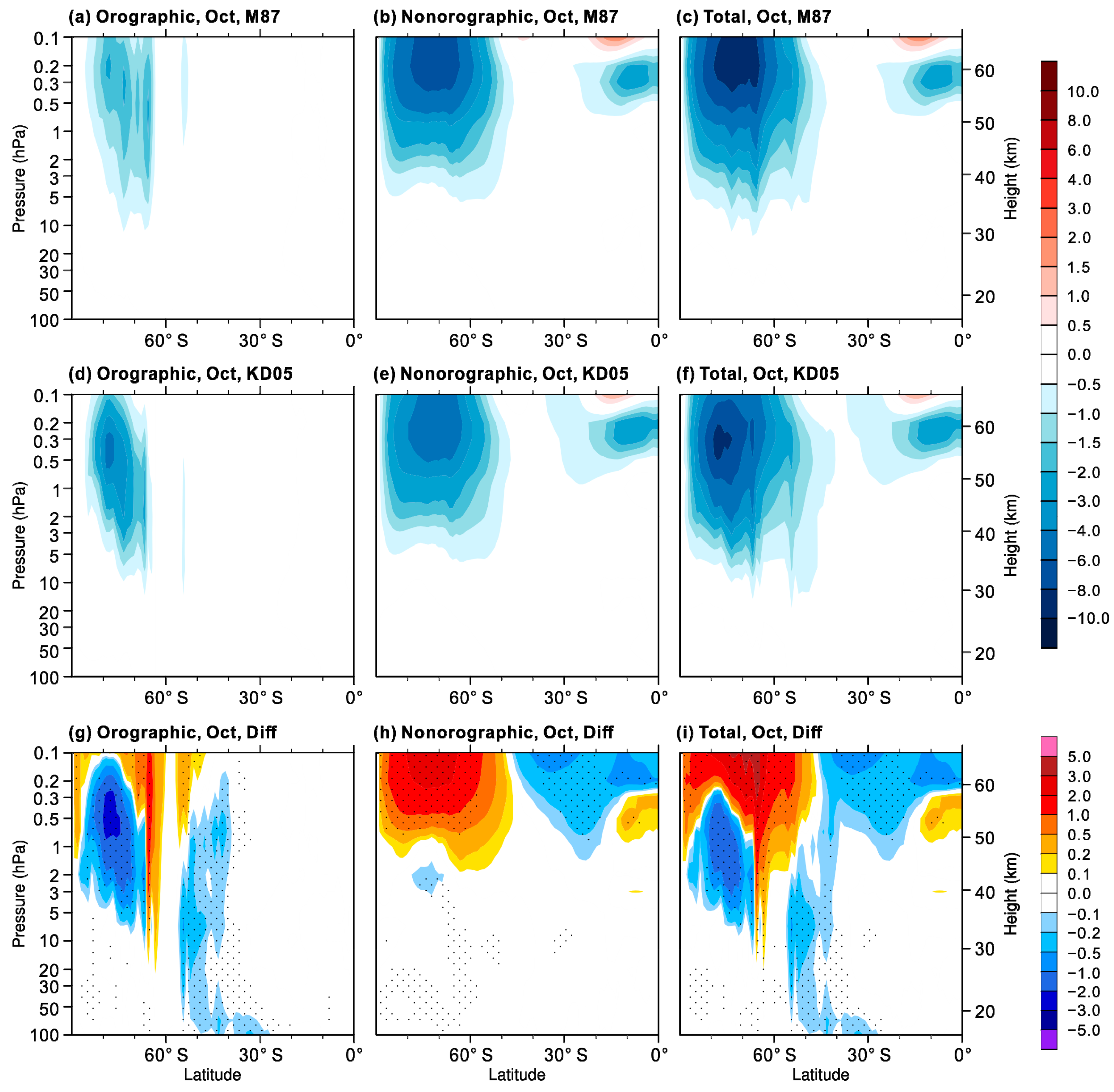
The cold-pole bias in the M87 simulation is significant. Figure 1 presents a comparison of Antarctic temperature averaged over the polar cap (60°–90° S) between the M87 simulation and JRA-55 reanalysis data. Figure 1a shows the JRA-55 daily climatology in the period of 1979–2012, and Figure 1b shows the difference between M87 and JRA-55. Stippled areas in this and similar comparisons denote differences that are statistically significant at the 95% confidence level, computed using a Student’s t test. The cold bias, which descends from the upper to the lower stratosphere in Antarctic late winter to spring (August–November), ranges from about −2 K to −8 K being significant at the 95% level, associated with the delayed breakdown of the stratospheric polar vortex in the M87 simulation. Results from KD05 present a roughly similar bias (Figure 1c). In detail, the modification of the orographic gravity wave parameterization has a remarkable influence on the temperature climatology in the Southern Hemisphere. Figure 1d shows the difference in the seasonal cycle of polar cap temperature between KD05 and M87. From August through November, much of the systematic cold bias has been reduced in KD05 by more than 2 K compared to M87. These differences between KD05 and M87 are significant at the 95% level. The remaining cold bias indicates that, despite the remarkable improvement of the temperature climatology, the breakdown of the southern polar vortex in the stratosphere still lags the observed behavior. Note that the comparisons shown in Figure 1b, 1c, and 1d are based on daily climatological averages for the period 1979–2012, and present sub-month perturbations which are closely associated with planetary wave modulation.
Some recent studies have reported the alleviation of the cold-pole bias [10,11]. For example, McLandress et al. (2012) [11] showed that the Southern Hemisphere cold-pole bias was reduced substantially by introducing an ad hoc source of additional orographic GWs centered on 60° S in the Canadian Middle Atmosphere Model. However, in the present study we have merely replaced the existing McFarlane (1987) [22] orographic GWD scheme by the Kim and Doyle (2005) [29] scheme in the BCC-AGCM, without attempting to address specifically the missing orographic GWD near 60° S where both schemes present the forcing gap as shown below.
Figure 2 compares the seasonal cycle of the zonal mean zonal wind at subpolar latitudes (55°–65° S) from the JRA-55 reanalysis data and simulations of M87 and KD05. The high wind bias in M87 is statistically significant. Above about 30 km, the zonal mean zonal wind is stronger in midwinter (June–July) by as much as 35 m s−1 in M87 compared to JRA-55 (Figure 2b). In spring and early summer (September–December), the zonal wind in M87 is stronger than JRA-55 by more than 20 m s-1, corresponding to the low temperature bias in this period, as shown in Figure 1b. Note also that the reversal of the zonal wind at 20 hPa, from westerly to easterly, occurs in JRA-55 in late November (Figure 2a) but is delayed in M87 until mid-December (Figure 2c). The zero-wind line just reaches the 30-hPa level in M87, whereas it is far below the 30-hPa level in the JRA-55 reanalysis data. Figure 2d shows the difference in the seasonal cycle of subpolar zonal wind between KD05 and JRA-55. While significant differences remain, much of the systematic high wind bias has been removed. During the transition from austral winter to summer in KD05, the high wind bias is reduced by more than 4 m s−1 compared to the M87 simulation, with these differences being significant at the 95% confidence level (Figure 2f). It can be expected that the date of the transition to easterlies is improved, indicated by the weaker winds in November in KD05.
Figure 3 presents a complementary view of the zonal wind evolution in the austral spring, exhibiting the monthly zonal mean zonal wind for September, October, and November in JRA-55, M87, and KD05. Significant differences can be seen between M87 and JRA-55, such as a stratospheric jet that is up to 20 m s−1 stronger in M87 than in JRA-55 between 100 and 1 hPa in September and October. The right column of Figure 3 shows the December–February seasonal average of the zonal-mean zonal wind. Apart from the weaker subtropical jet in the Northern Hemisphere, M87 performs reasonably well in the austral summer. Also note that the stratospheric polar-night jet simulated in M87 is stronger and more upright than that in JRA-55, leading to a shift in the position of the simulated polar vortex in boreal winter. Inclusion of the modified orographic GW parameterization results in better agreement between KD05 and JRA-55. The austral spring stratospheric jet is much weaker in KD05, especially in September and October, when the differences between the simulated and observed winds are reduced to about 10 m s−1. In the austral summer (December–February, Figure 3l), it is interesting to note that the Southern Hemisphere winds in KD05 are very similar to those in M87, while the Northern Hemisphere winds are improved, as shown by a stronger subtropical jet which is closer to the reanalysis data.
The improved simulation of the breakdown of the Southern Hemisphere stratospheric polar vortex is better illustrated in Figure 4, which shows the mean final warming dates at 50 hPa. Following Black and McDaniel (2007) [32], 5-day running means of daily data are used to calculate the final warming date as the final time that the zonal mean zonal wind at 60° S and 50 hPa drops below 10 m s−1 and remains below that value through the following summer. The mean final warming date for the M87 simulation is about 24 days later than that for JRA-55, which is consistent with the results shown in Figure 3. The final warming dates in the KD05 experiment are about 8 days earlier than in the M87 experiment and are now in closer agreement with JRA-55. Results from McLandress et al. (2012) [11] and de la Cámara et al. (2016) [12] are also included in Figure 4 for reference. Both works achieved bigger improvements in the delayed final warming dates, while large discrepancies between KD05 and JRA-55 exist. The most likely cause for this difference is that the middle-atmosphere configuration of BCC-AGCM with the Kim and Doyle (2005) scheme still underestimates the GW forcing in the southern stratosphere, particularly around 60° S.

3.2. Changes in GWD

Figure 5 shows the latitude-height cross sections of orographic, nonorographic, and total GWD in the M87 and KD05 experiments for October, focusing on stratospheric levels from 100 to 0.1 hPa in the Southern Hemisphere. Overall, the distributions of the parameterized GWD in the two experiments are similar. The orographic GWD parameterized using the schemes of McFarlane (1987) [22] and Kim and Doyle (2005) [29], respectively, mainly occurs above 10 hPa in high latitudes. The gap in orographic GWD near 60° S is present in both experiments, consistent with the absence of topography in that latitude band. Compared with M87, significant orographic GWD enhancement in KD05 is found in the upper stratosphere over the Antarctic continent, along with moderate orographic GWD increase in the middle and lower stratosphere between 30° and 60° S where large mountains exist. On the other hand, the nonorographic GWD spreads out over a wider latitudinal region and generally increases with increasing height above 5 hPa in the mid to high latitudes with a latitudinal maximum around 70° S in the M87 and KD05 experiments. In contrast to the orographic GWs, the parameterized nonorographic GWs exert a strong drag on the zonal winds near 60° S. Although the nonorographic GWD in the two experiments is obtained from the same parameterization schemes, it weakens in the higher latitudes and strengthens in the lower latitudes above 1 hPa in KD05, probably because of the changes in the zonal-mean zonal winds induced by the enhanced orographic GWD. As a result, the changes in total GWD, i.e., the sum of orographic and nonorographic GWD, are dominated by orographic drag below about 1 hPa and nonorographic drag above 1 hPa.
It should be noted that the parameterized nonorographic GWD largely contributes to the total GWD in the stratosphere during the austral spring, both in the M87 and KD05 experiments. This differs from most climate models, in which the orographic GWD is much stronger than the nonorographic GWD. For example, McLandress (2012) found that the orographic GWD far outweighs the nonorographic GWD in the Canadian Middle Atmosphere Model and the Southern Hemisphere cold-pole bias was reduced when including an extra drag at 60° S in the orographic GWD scheme [11]. Uncertainties in the relative contribution of the nonorographic and orographic GWD to the total GWD come mainly from diverse constructions of nonorographic GWD parameterization in climate models. While the parameterization of GWs due to orography is relatively well understood, the GWs emitted by convection, fronts, and jets are often represented using uniform sources [33,34,35]. Source-related nonorographic GWD parameterizations may be more valid in modeling studies of the relative contribution of each GW during the southern SFW.

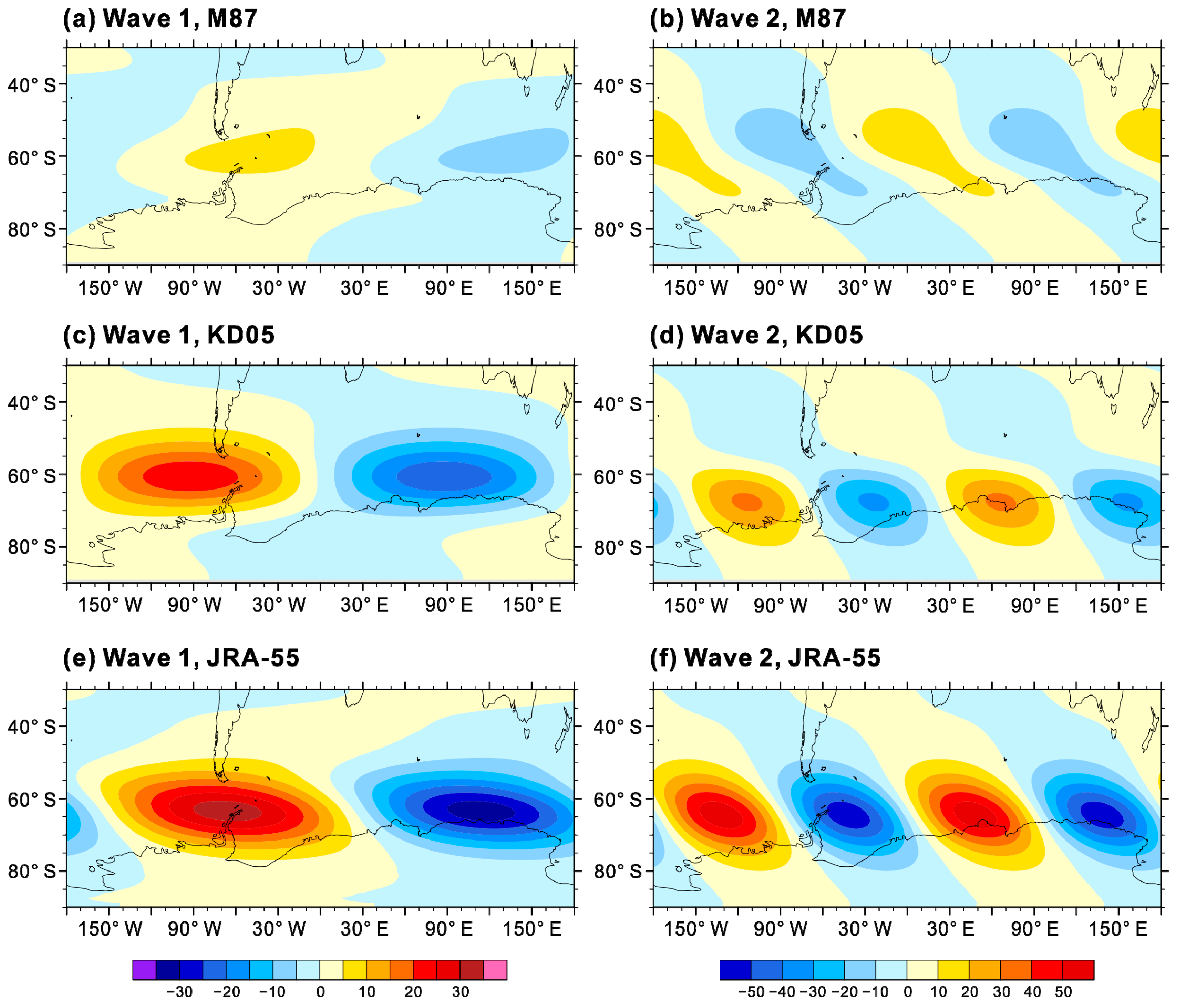
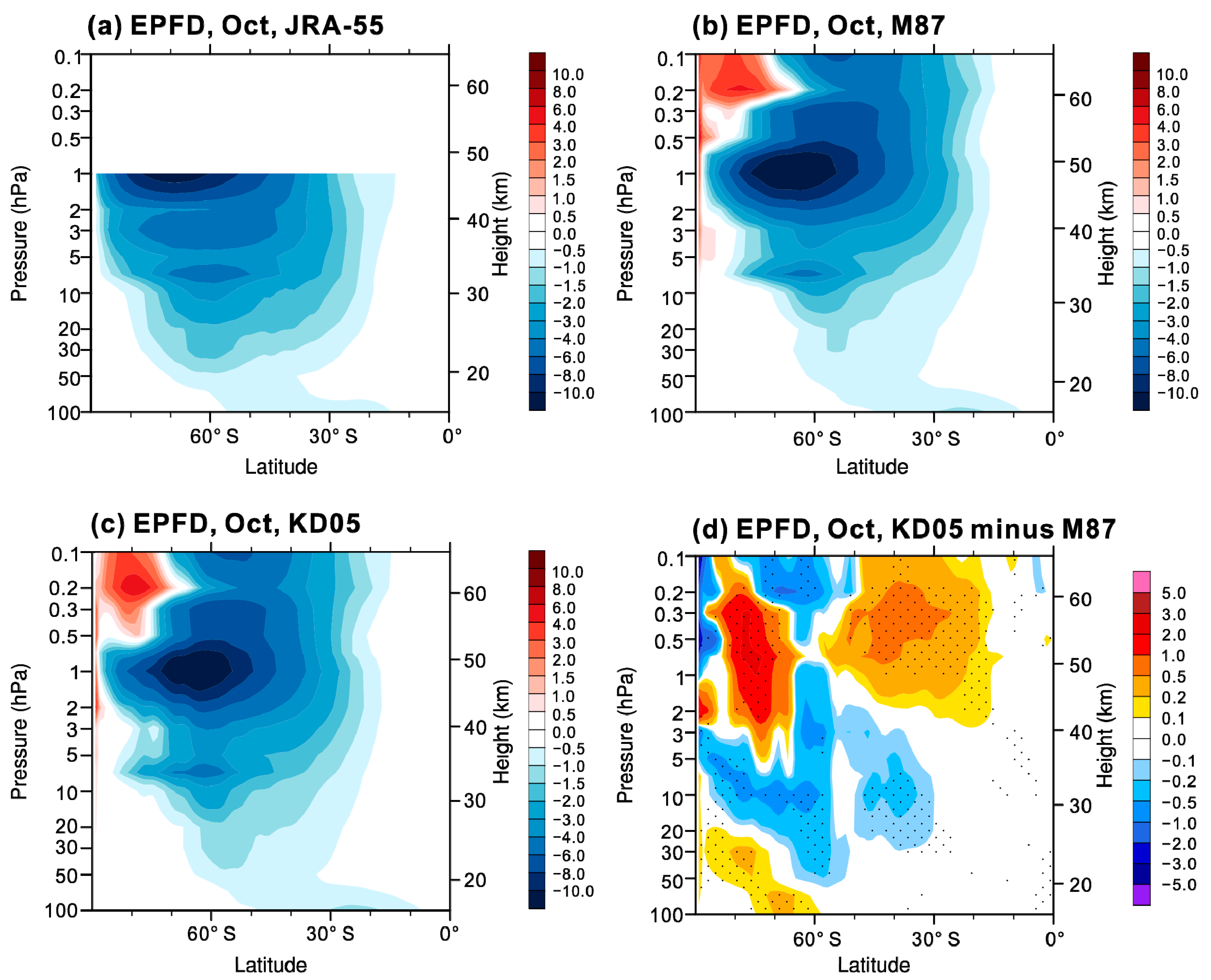
3.3. Resolved Wave Forcing Responses

The resolved wave flux from the troposphere was first examined, as shown by the 100-hPa meridional heat flux at Southern Hemisphere high latitudes for October (Figure 6). It is clear that both waves 1 and 2 are improved significantly in KD05, indicating tropospheric wave forcing of the stratosphere is in closer agreement with JRA-55. Figure 7 shows latitude-height cross sections of monthly mean resolved wave forcing, i.e., divergence of the E-P flux, in M87 and KD05 for October throughout the southern stratosphere. As shown in JRA-55, the resolved wave drag is spread out over a wide latitudinal range, with a maximum around 1 hPa in the high latitudes (Figure 7a). Overall, the latitude-height distribution of the resolved wave forcing is reasonably reproduced in M87 (Figure 7b). The magnitude and the extent of the negative wave forcing in KD05 resembles that in M87 (Figure 7b,c). However, changes in the resolved wave drag in the stratosphere do occur due to changes in the parameterized GWD. Compared with M87, E-P flux divergence in KD05 becomes more negative in the lower stratosphere and more positive in the upper stratosphere. Furthermore, a notable feature in the difference of E-P flux divergence is that there is a tongue of stronger wave forcing at 60° S in KD05 (Figure 7d). These differences are generally significant at the 95% confidence level.

3.4. Total Wave Forcing

Figure 8 shows the change in total wave forcing (GWD plus E-P flux divergence). Consistent with previous studies [36], changes in GWD are accompanied by changes in the E-P flux divergence of resolved waves such that partial compensation occurs between the two. One piece of evidence is that the negative changes in resolved wave drag above 1 hPa around 60° S (Figure 7d) coincide with the positive changes in GWD in this region (Figure 5i). The compensation between different sources of mechanical forcing results in a much smoother latitudinal distribution of changes in total wave forcing than in GWD or E-P flux divergence individually. Figure 8 suggests that the reduced wave forcing in the upper stratosphere comes mainly from nonorographic GWD and resolved wave drag, whereas the enhanced wave forcing comes primarily from orographic GWD and resolved wave drag. A sharp decrease in total wave forcing is present around 66° S. This corresponds to the abrupt decrease in the orographic GWD within grid cells of sharp topographic features surrounded by oceans, as seen in Figure 5g. The monthly mean annual cycle of the differences in the total wave forcing between the two experiments is presented in Figure 9. From August through November, the negative total wave forcing is strengthened in KD05, corresponding to the reduced cold bias as shown in Figure 1c.

3.5. Polar Downwelling in the Southern Hemisphere

We consider next how the changes in wave forcing documented above affect downwelling (and hence temperature) at high latitudes of the Southern Hemisphere. Figure 10 shows the vertical component of the residual mean meridional circulation averaged over the Southern Hemisphere polar cap for M87 and KD05 simulations, and their difference. Compared to M87, the warming in early spring and the cooling in late spring (Figure 1c) are a consequence of enhanced and reduced downwelling in KD05, respectively (Figure 10d). The anomalous downwelling and upwelling are driven by the enhanced and reduced wave forcing, as seen in Figure 9. Note that anomalous upwelling locates at ~0.5–3 hPa around June–August, which may be associated with reduced nonorographic GWD or resolved wave drag in the upper southern stratosphere.

4. Summary and Conclusions

It is shown in this study that modifying the orographic GW parameterization results in an improved simulation of the SFW over Antarctica. A pair of experiments were conducted to compare two orographic GW schemes, namely, the McFarlane (1987) [22] scheme and the Kim and Doyle (2005) [29] scheme, in modeling the breakdown of the stratospheric polar vortex over Antarctica. The cold-pole bias is reduced by more than 2 K and the associated high wind bias is reduced by more than 4 m s−1 when the McFarlane (1987) [22] scheme is replaced by the Kim and Doyle (2005) [29] scheme. Correspondingly, the delayed SFW can be alleviated by 8 days. Further investigations on the wave forcing show that the improvements come from the accelerated downwelling branch of the BDC in the lower stratosphere, which in turn is mainly driven by the enhanced orographic GWD. This study suggests that modifying existing orographic GWD parameterizations would be a valid way of improving the SFW simulation over Antarctica.
Current representation of orographic GWD in climate models has been developed to a relatively complex level but still has uncertain formulation details. This study demonstrates that a more recent orographic GWD parameterization can go a long way in improving the cold-pole bias to a certain extent. However, comparing with statistics from the previous studies reveals that simply changing the parameterization schemes results in limited improvements compared to those that would be attained by adding a missing drag around 60° S. The absent orographic GWD near 60° S may be due to the simplified assumption that mountain waves only propagate vertically within the model grid column where they are triggered. The horizontal propagate of mountain waves is not taken into account in any traditional orographic GWD scheme. Recently, new orographic GW parameterizations considering horizontal wave propagation have been proposed and present significant impacts on the orographic GWD distribution [37,38]. Including the horizontal propagation effects of orographic GWs may lead to a much-improved cold-bias in climate models.
The general consensus to explain the delayed SFW over Antarctica is that climate models underestimate the GW forcing in the southern stratosphere, but the orographic or nonorographic origin of the insufficient GW drag is still controversial. Similar to orographic GWs, nonorographic GWs also act to drive the downwelling branch of the BDC. Observational studies have found that GWs over the ocean surrounding Antarctica are highly related to nonorographic sources [39,40,41,42]. Furthermore, the role of nonorographic GWs has been examined in modeling studies and it was found that parameterized GWs emitted by fronts and jets contribute significantly to the simulated Antarctic stratospheric vortex [10,12]. The effect of improving the representation of nonorographic GWs on the simulated southern SFW in climate models is beyond the scope of this paper and will be explored in future work.

Author Contributions

Conceptualization, Y.L. and T.W.; methodology, Y.L. and X.X.; software, Y.L., T.W. and X.X.; validation, Y.L. and X.X.; formal analysis, Y.L.; investigation, Y.L.; data curation, Y.L.; writing—original draft preparation, Y.L.; writing—review and editing, L.Z. and M.C.; visualization, Y.L.; supervision, Y.L.; project administration, T.W. All authors have read and agreed to the published version of the manuscript.

Funding

This work was supported by the National Key Research and Development Program of China (2016YFA0602100). Xin Xu was supported by the Numerical Model Development Project of China Meteorological Administration (QHMS2019006). Min Chu was supported by the National Key Research and Development Program of China (2018YFC1407104).

Acknowledgments

We gratefully acknowledge the group of the JRA-55 reanalysis (https://jra.kishou.go.jp/JRA-55) for providing public access. All the graphics in this paper were created by the NCAR Command Language (NCL; doi:10.5065/D6WD3XH5). The authors are grateful to the editor and the three anonymous reviewers for their careful work and valuable comments that helped to improve the manuscript.

Conflicts of Interest

The authors declare no conflict of interest.

References

  1. Morgenstern, O.; Hegglin, M.I.; Rozanov, E.; O’Connor, F.M.; Abraham, N.L.; Akiyoshi, H.; Archibald, A.T.; Bekki, S.; Butchart, N.; Chipperfield, N.P.; et al. Review of the global models used within phase 1 of the Chemistry-Climate Model Initiative (CCMI). Geosci. Model Dev. 2017, 10, 639–671. [Google Scholar] [CrossRef] [Green Version]
  2. Morgenstern, O.; Giorgetta, M.A.; Shibata, K.; Eyring, V.; Waugh, D.W.; Shepherd, T.G.; Akiyoshi, H.; Austin, J.; Baumgaertner, A.J.G.; Bekki, S.; et al. Review of the formulation of present-generation chemistry-climate models and associated forcings. J. Geophys. Res. 2010, 115, D00M02. [Google Scholar] [CrossRef] [Green Version]
  3. Eyring, V.; Butchart, N.; Waugh, D.W.; Akiyoshi, H.; Austin, J.; Bekki, S.; Bodeker, G.E.; Boville, B.A.; Brühl, C.; Chipperfield, M.P.; et al. Assessment of temperature, trace species and ozone in chemistry-climate model simulations of the recent past. J. Geophys. Res. 2006, 111, D22308. [Google Scholar] [CrossRef]
  4. Eyring, V.; Shepherd, T.G.; Waugh, D.W. SPARC report on the evaluation of chemistry-climate models. SPARC Tech. Rep. 2010, 5, 425. [Google Scholar]
  5. Wilcox, L.J.; Charlton-Perez, A.J. Final warming of the Southern Hemisphere polar vortex in high- and low-top CMIP5 models. J. Geophys. Res. Atmos. 2013, 118, 2535–2546. [Google Scholar] [CrossRef] [Green Version]
  6. Butchart, N.; Charlton-Perez, A.J.; Cionni, I.; Hardiman, S.C.; Haynes, P.H.; Krüger, K.; Kushner, P.J.; Newman, P.A.; Osprey, S.M.; Perlwitz, J.; et al. Multimodel climate and variability of the stratosphere. J. Geophys. Res. 2011, 116, D05102. [Google Scholar] [CrossRef] [Green Version]
  7. Stolarski, R.S.; Douglass, A.R.; Gupta, M.; Newman, P.A.; Pawson, S.; Schoeberl, M.R.; Nielsen, J.E. An ozone increase in the Antarctic summer stratosphere: A dynamical response to the ozone hole. Geophys. Res. Lett. 2006, 33, L21805. [Google Scholar] [CrossRef]
  8. Sun, L.; Chen, G.; Robinson, W.A. The role of stratospheric polar vortex breakdown in Southern Hemisphere climate trends. J. Atmos. Sci. 2014, 71, 2335–2353. [Google Scholar] [CrossRef]
  9. Barnes, E.A.; Barnes, N.W.; Polvani, L.M. Delayed Southern Hemisphere climate change induced by stratospheric ozone recovery, as projected by the CMIP5 models. J. Clim. 2014, 27, 852–867. [Google Scholar] [CrossRef] [Green Version]
  10. Garcia, R.R.; Smith, A.K.; Kinnison, D.E.; de la Cámara, A.; Murphy, D.J. Modification of the gravity wave parameterization in the Whole Atmosphere Community Climate Model: Motivation and results. J. Atmos. Sci. 2017, 74, 275–291. [Google Scholar] [CrossRef]
  11. McLandress, C.; Shepherd, T.G.; Polavarapu, S.; Beagley, S.R. Is missing orographic gravity wave drag near 60 °S the cause of the stratospheric zonal wind biases in chemistry-climate models? J. Atmos. Sci. 2012, 69, 802–818. [Google Scholar] [CrossRef] [Green Version]
  12. De la Cámara, A.; Lott, F.; Jewtoukoff, V.; Plougonven, R.; Hertzog, A. On the gravity wave forcing during the southern stratospheric final warming in LMDZ. J. Atmos. Sci. 2016, 73, 3213–3226. [Google Scholar] [CrossRef]
  13. Sato, K.; Yasui, R.; Miyoshi, Y. The momentum budget in the stratosphere, mesosphere, and lower thermosphere. Part I: Contribution of different wave types and in situ generation of Rossby waves. J. Atmos. Sci. 2018, 75, 3613–3633. [Google Scholar] [CrossRef]
  14. Yasui, R.; Sato, K.; Miyoshi, Y. The momentum budget in the stratosphere, mesosphere, and lower thermosphere. Part II: The in situ generation of gravity waves. J. Atmos. Sci. 2018, 75, 3635–3651. [Google Scholar] [CrossRef]
  15. Sato, K.; Hirano, S. The climatology of the Brewer-Dobson circulation and the contribution of gravity waves. Atmos. Chem. Phys. 2019, 19, 4517–4539. [Google Scholar] [CrossRef] [Green Version]
  16. Scheffler, G.; Pulido, M. Estimation of gravity-wave parameters to alleviate the delay in the Antarctic vortex breakup in general circulation models. Q. J. R. Meteorol. Soc. 2017, 143, 2157–2167. [Google Scholar] [CrossRef] [Green Version]
  17. Alexander, M.J.; Eckermann, S.D.; Broutman, D.; Ma, J. Momentum flux estimates for South Georgia Island mountain waves in the stratosphere observed via satellite. Geophys. Res. Lett. 2009, 36, L12816. [Google Scholar] [CrossRef] [Green Version]
  18. Alexander, M.J.; Grimsdell, A.W. Seasonal cycle of orographic gravity wave occurrence above small islands in the Southern Hemisphere: Implications for effects on the general circulation. J. Geophys. Res. Atmos. 2013, 118, 11589–11599. [Google Scholar] [CrossRef]
  19. Sato, K.; Watanabe, S.; Kawatani, Y.; Tomikawa, Y.; Miyazaki, K.; Takahashi, M. On the origins of mesospheric gravity waves. Geophys. Res. Lett. 2009, 36, L19801. [Google Scholar] [CrossRef] [Green Version]
  20. Sato, K.; Tateno, S.; Watanabe, S.; Kawatani, Y. Gravity wave characteristics in the Southern Hemisphere revealed by a high resolution middle-atmosphere general circulation model. J. Atmos. Sci. 2012, 69, 1378–1396. [Google Scholar] [CrossRef]
  21. Hindley, N.P.; Wright, C.J.; Smith, N.D.; Mitchell, N.J. The southern stratospheric gravity wave hot spot: Individual waves and their momentum fluxes measured by COSMIC GPS-RO. Atmos. Chem. Phys. 2015, 15, 7797–7818. [Google Scholar] [CrossRef] [Green Version]
  22. McFarlane, N.A. The effect of orographically excited wave drag on the general circulation of the lower stratosphere and troposphere. J. Atmos. Sci. 1987, 44, 1775–1800. [Google Scholar] [CrossRef] [Green Version]
  23. Beres, J.H.; Alexander, M.J.; Holton, J.R. A method of specifying the gravity wave spectrum above convection based on latent heating properties and background wind. J. Atmos. Sci. 2004, 61, 324–337. [Google Scholar] [CrossRef] [Green Version]
  24. De la Cámara, A.; Lott, F. A stochastic parameterization of the gravity waves emitted by fronts and jets. Geophys. Res. Lett. 2015, 42, 2071–2078. [Google Scholar] [CrossRef]
  25. Wu, T.; Lu, Y.; Fang, Y.; Xin, X.; Li, L.; Li, W.; Jie, W.; Zhang, J.; Liu, Y.; Zhang, L.; et al. The Beijing Climate Center Climate System Model (BCC-CSM): The main progress from CMIP5 to CMIP6. Geosci. Model Dev. 2019, 12, 1573–1600. [Google Scholar] [CrossRef] [Green Version]
  26. Lu, Y.; Wu, T.; Jie, W.; Scaife, A.A.; Andrews, M.B.; Richter, J.H. Variability of the stratospheric quasi-biennial oscillation and its wave forcing simulated in the Beijing Climate Center Atmospheric General Circulation Model. J. Atmos. Sci. 2020, 77, 149–165. [Google Scholar] [CrossRef]
  27. Richter, J.H.; Sassi, F.; Garcia, R.R. Toward a physically based gravity wave source parameterization in a general circulation model. J. Atmos. Sci. 2010, 67, 136–156. [Google Scholar] [CrossRef]
  28. Lindzen, R.S. Turbulence and stress owing to gravity wave and tidal breakdown. J. Geophys. Res. 1981, 86, 9707–9714. [Google Scholar] [CrossRef] [Green Version]
  29. Kim, Y.-J.; Doyle, J.D. Extension of an orographic drag parametrization scheme to incorporate orographic anisotropy and flow blocking. Q. J. R. Meteorol. Soc. 2005, 131, 1893–1921. [Google Scholar] [CrossRef] [Green Version]
  30. Kobayashi, S.; Ota, Y.; Harada, Y.; Ebita, A.; Moriya, M.; Onoda, H.; Onogi, K.; Kamahori, H.; Kobayashi, C.; Endo, H.; et al. The JRA-55 reanalysis: General specifications and basic characteristics. J. Meteorol. Soc. Jpn. 2015, 93, 5–48. [Google Scholar] [CrossRef] [Green Version]
  31. Andrews, D.G.; Holton, J.R.; Leovy, C.B. Middle Atmosphere Dynamics; Academic Press: Cambridge, MA, USA, 1987; p. 489. [Google Scholar]
  32. Black, R.W.; McDaniel, B.A. Interannual variability in the Southern Hemisphere circulation organized by stratospheric final warming events. J. Atmos. Sci. 2007, 64, 2968–2974. [Google Scholar] [CrossRef]
  33. Warner, C.D.; McIntyre, M.E. On the propagation and dissipation of gravity wave spectra through a realistic middle atmosphere. J. Atmos. Sci. 1996, 53, 3213–3235. [Google Scholar] [CrossRef] [Green Version]
  34. Hines, C.O. Doppler-spread parameterization of gravity-wave momentum deposition in the middle atmosphere. Part I: Basic formulation. J. Atmos. Sol.-Terr. Phys. 1997, 59, 371–386. [Google Scholar] [CrossRef]
  35. Scinocca, J.F. An accurate spectral non-orographic gravity wave parameterization for general circulation models. J. Atmos. Sci. 2003, 60, 667–682. [Google Scholar] [CrossRef]
  36. Scheffler, G.; Pulido, M. Compensation between resolved and unresolved wave drag in the stratospheric final warmings of the Southern Hemisphere. J. Atmos. Sci. 2015, 72, 4393–4411. [Google Scholar] [CrossRef]
  37. Xu, X.; Song, J.J.; Wang, Y.; Xue, M. Quantifying the effect of horizontal propagation of three-dimensional mountain waves on the wave momentum flux using Gaussian beam approximation. J. Atmos. Sci. 2017, 74, 1783–1798. [Google Scholar] [CrossRef]
  38. Xu, X.; Wang, Y.; Xue, M.; Zhu, K. Impacts of horizontal propagation of orographic gravity waves on the wave drag in the stratosphere and lower mesosphere. J. Geophys. Res. Atmos. 2017, 122, 11301–11312. [Google Scholar] [CrossRef]
  39. Plougonven, R.; Hertzog, A.; Guez, L. Gravity waves over Antarctica and the Southern Ocean: Consistent momentum fluxes in mesoscale simulations and stratospheric balloon observations. Quart. J. Roy. Meteor. Soc. 2013, 139, 101–118. [Google Scholar] [CrossRef]
  40. Hendricks, E.A.; Doyle, J.D.; Eckermann, S.D.; Jiang, Q.; Reinecke, P.A. What is the source of the stratospheric gravity wave belt in austral winter? J. Atmos. Sci. 2014, 71, 1583–1592. [Google Scholar] [CrossRef]
  41. Jewtoukoff, V.; Hertzog, A.; Plougonven, R.; de la Cámara, A.; Lott, F. Gravity waves in the Southern Hemisphere derived from balloon observations and the ECMWF analyses. J. Atmos. Sci. 2015, 72, 3449–3468. [Google Scholar] [CrossRef]
  42. Shibuya, R.; Sato, K.; Tomikawa, Y.; Tsutsumi, M.; Sato, T. A study of multiple tropopause structures caused by inertia-gravity waves in the Antarctic. J. Atmos. Sci. 2015, 72, 2109–2130. [Google Scholar] [CrossRef]
Figure 1. (a) Climatological seasonal cycle of Antarctic polar cap (60°–90° S) temperature (K) from JRA-55 daily data; (b) difference between M87 and JRA-55; (c) difference between KD05 and JRA-55; and (d) difference between KD05 and M87. Stippling denotes differences are statistically significant at the 95% confidence level.
Atmosphere 11 00576 g001
Figure 2. Seasonal cycle of daily zonal-mean zonal wind averaged over southern subpolar latitudes (55° S–65° S) in (a) the JRA-55 reanalysis, (c) the M87 simulation and (e) the M87 simulation. (b) Difference between M87 and JRA-55. (d) Difference between KD05 and JRA-55. (f) Difference between KD05 and M87. The thick dashed line denotes the zero-wind contour. Stippling denotes differences are statistically significant at the 95% confidence level.
Atmosphere 11 00576 g002
Figure 3. Latitude-height cross sections of zonal-mean zonal wind (m s−1) in (ad) JRA-55, (eh) M87, and (il) KD05 for (a,e,i) September, (b,f,j) October, (c,g,k) November, and (d,h,l) December–February. Contour interval is 10 m s−1. Zero winds are denoted by the black thick lines.
Atmosphere 11 00576 g003
Figure 4. Mean final warming dates at 50 hPa for the M87 experiment (red), KD05 experiment (blue), and JRA-55 reanalysis (black) for 1979–2012. The final warming date is here defined by when the zonal mean zonal wind at 60° S and 50 hPa drops below 10 m s−1 and remains so for the duration of the summer. Results from McLandress et al. (2012) [11] and de la Cámara et al. (2016) [12] are included for reference.
Atmosphere 11 00576 g004
Figure 5. Latitude-height cross sections in the stratosphere of (a,d) orographic, (b,e) nonorographic, and (c,f) total GWD (m s−1 day−1) in the M87 and KD05 experiments for October. Differences (KD05 minus M87) in gravity wave drag are shown in (gi). Total GWD is the sum of the orographic and nonorographic GWD. Stippling denotes differences are statistically significant at the 95% confidence level.
Atmosphere 11 00576 g005
Figure 6. Distribution of the 100-hPa meridional heat flux (K m s−1) by the zonal wave number 1 (a,c,e) and zonal wave number 2 (b,d,f) at Southern Hemisphere high latitudes for October.
Atmosphere 11 00576 g006
Figure 7. Resolved wave forcing (m s−1 day−1) in (a) JRA-55, (b) M87, (c) KD05, and (d) the differences between KD05 and M87 for October. Resolved wave forcing is expressed by the Eliassen–Palm flux divergence (EPFD). Stippling denotes differences are statistically significant at the 95% confidence level.
Atmosphere 11 00576 g007
Figure 8. Difference (KD05 minus M87) in total wave forcing (m s−1 day−1) for October. Total wave drag is the sum of the resolved wave drag and total GWD. Stippling denotes differences are statistically significant at the 95% confidence level.
Atmosphere 11 00576 g008
Figure 9. Climatological seasonal cycle (1979−2012) of monthly difference (KD05 minus M87) in total wave forcing (m s−1 day−1) averaged over the southern midlatitudes (40°–80° S). Stippling denotes differences are statistically significant at the 95% confidence level.
Atmosphere 11 00576 g009
Figure 10. Climatological seasonal cycle (1979–2012) of monthly residual vertical velocity (mm s−1) averaged over the southern polar cap (60°–90° S) in (a) JRA-55, (b) M87, (c) KD05, and (d) difference between KD05 and M87. Stippling denotes differences are statistically significant at the 95% confidence level.
Atmosphere 11 00576 g010
Table 1. Summary of experimental setups.
Run NameOrographic GWsNonorographic GWs
M87McFarlane (1987)Beres et al. (2004) [23]; de la Cámara and Lott (2015) [24]
KD05Kim and Doyle (2005)Beres et al. (2004) [23]; de la Cámara and Lott (2015) [24]

