Structure of Approximate Roots Based on Symmetric Properties of (p, q)-Cosine and (p, q)-Sine Bernoulli Polynomials

Abstract

This paper constructs and introduces $(p,q)$-cosine and $(p,q)$-sine Bernoulli polynomials using $(p,q)$-analogues of ${(x+a)}^n$. Based on these polynomials, we discover basic properties and identities. Moreover, we determine special properties using $(p,q)$-trigonometric functions and verify various symmetric properties. Finally, we check the symmetric structure of the approximate roots based on symmetric polynomials.

1. Introduction

In 1991, $(p,q)$-calculus including $(p,q)$-number with two independent variables p and q, was first independently considered [1,2]. Throughout this paper, the sets of natural numbers, integers, real numbers and complex numbers are denoted by $\mathbb{N},\mathbb{Z},\mathbb{R}$ and $\mathbb{C}$, respectively.

For any $n\in \mathbb{N}$, the $(p,q)$-number is defined by the following:

$${\left[n\right]}_{p,q}=\frac{p^n-q^n}{p-q},\mathrm{where}|p/q|<1,$$

(1)

which is a natural generalization of the q-number. From Equation (1), we note that ${\left[n\right]}_{p,q}={\left[n\right]}_{q,p}$.

Many physical and mathematical problems have led to the necessity of studying $(p,q)$-calculus. Since 1991, many mathematicians and physicists have developed $(p,q)$-calculus in several different research areas. For example, in 1994, [3] introduced $(p,q)$-hypergeometric functions. Three years later, [3,4] derived related preliminary results by considering a more general $(p,q)$-hypergeometric series and Burban’s $(p,q)$-hypergeometric series, respectively. In 2005, based on the $(p,q)$-numbers, [5] studied about $(p,q)$-hypergeometric series and discovered results corresponding to the $(p,q)$-extensions of known q-identities. Moreover, [6] established properties similar to the ordinary and q-binomial coefficients after developing the $(p,q)$-hypergeometric series in 2008. About seven years later, [7] introduced $(p,q)$-gamma and $(p,q)$-beta functions, which are generalizations of the gamma and beta functions.

The different variations of Bernoulli polynomials, q-Bernoulli polynomials and $(p,q)$-Bernoulli polynomials are illustrated in the diagram below. Kim, Ryoo and many mathematicians have studied the first and second rows of the polynomials in the diagram (see [8,9,10,11,12]). These studies began producing valuable results in areas related to number theory and combinatorics.

The main idea is to use property of $(p,q)$-numbers and combine $(p,q)$-trigonometric functions. From this idea, we construct $(p,q)$-cosine and $(p,q)$-sine Bernoulli polynomials. Investigating the various explicit identities for $(p,q)$-cosine and $(p,q)$-sine Bernoulli polynomials in the diagram’s third row is the main goal of this paper.

Due to their importance, the classical Bernoulli, Euler, and Genocchi polynomials have been studied extensively and are well-known. Mathematicians have studied these polynomials through various mathematical applications including finite difference calculus, p-adic analytic number theory, combinatorial analysis and number theory. Many mathematicians are familiar with the theorems and definitions of classical Bernoulli, Euler, and Genocchi polynomials. Based on the theorems and definitions, it is significant to study these properties in various ways by the combining with Bernoulli, Euler, and Genocchi polynomials. Mathematicians are studying the extended versions of these polynomials and are researching new polynomials by combining mathematics with other fields, such as physics or engineering (see [9,10,11,12,13,14]). The definition of Bernoulli polynomials combined with $(p,q)$-numbers follows:

Definition 1.

The $(p,q)$-Bernoulli numbers, $B_{n,p,q}$, and polynomials, $B_{n,p,q}\left(z\right)$, can be expressed as follows (see [8])

$$\sum _{n=0}^{\infty }{B}_{n,p,q}\frac{t^n}{{\left[n\right]}_{p,q}!}=\frac{t}{e_{p,q}\left(t\right)-1},\sum _{n=0}^{\infty }{B}_{n,p,q}\left(z\right)\frac{t^n}{{\left[n\right]}_{p,q}!}=\frac{t}{e_{p,q}\left(t\right)-1}{e}_{p,q}\left(tz\right).$$

(2)

In [11], we confirmed the properties of q-cosine and q-sine Bernoulli polynomials. Their definitions and representative properties are as follows.

Definition 2.

The q-cosine Bernoulli polynomials ${}_C{B}_{n,q}(x,y)$ and q-sine Bernoulli polynomials ${}_S{B}_{n,q}(x,y)$ are defined by the following:

$$\sum _{n=0}^{\infty }{}_C{B}_{n,q}(x,y)\frac{t^n}{n!}=\frac{t}{e_q\left(t\right)-1}{e}_q\left(tx\right){\mathit{COS}}_q\left(ty\right),\sum _{n=0}^{\infty }{}_S{B}_n(x,y)\frac{t^n}{n!}=\frac{t}{e_q\left(t\right)-1}{e}_q\left(tx\right){\mathit{SIN}}_q\left(ty\right).$$

(3)

Theorem 1.

For $x,y\in \mathbb{R}$, we have the following:

$$\begin{array}{cc}\left(i\right)\hfill & \{\begin{array}{c}{}_C{B}_{n,q}({(x\oplus r)}_q,y)+{}_S{B}_{n,q}({(x\ominus r)}_q,y)\hfill \\ ={\sum }_{k=0}^n{\left[\begin{array}{c}n\\ k\end{array}\right]}_q{q}^{\left(\genfrac{}{}{0pt}{}{n-k}{2}\right)}{r}^{n-k}({}_C{B}_{k,q}(x,y)+{(-1)}^{n-k}{}_S{B}_{k,q}(x,y))\hfill \\ {}_S{B}_{n,q}({(x\oplus r)}_q,y)+{}_C{B}_{n,q}({(x\ominus r)}_q,y)\hfill \\ ={\sum }_{k=0}^n{\left[\begin{array}{c}n\\ k\end{array}\right]}_q{q}^{\left(\genfrac{}{}{0pt}{}{n-k}{2}\right)}{r}^{n-k}({}_S{B}_{k,q}(x,y)+{(-1)}^{n-k}{}_C{B}_{k,q}(x,y))\hfill \end{array}\hfill \\ \left(ii\right)\hfill & \{\begin{array}{c}\frac{\partial }{\partial x}{}_C{B}_{n,q}(x,y)={\left[n\right]}_q{}_C{B}_{n-1,q}(x,y),\frac{\partial }{\partial y}{}_C{B}_{n,q}(x,y)=-{\left[n\right]}_q{}_S{B}_{n-1,q}(x,qy)\hfill \\ \frac{\partial }{\partial x}{}_S{B}_{n,q}(x,y)={\left[n\right]}_q{}_S{B}_{n-1,q}(x,y),\frac{\partial }{\partial y}{}_S{B}_{n,q}(x,y)={\left[n\right]}_q{}_C{B}_{n-1,q}(x,qy)\hfill \end{array}\hfill \end{array}$$

(4)

The main goal of this paper is to identify the properties of $(p,q)$-cosine and $(p,q)$-sine Bernoulli polynomials. In Section 2, we review some definitions and theorem of $(p,q)$-calculus. In Section 3, we introduce $(p,q)$-cosine and $(p,q)$-sine Bernoulli polynomials. Using the properties of exponential functions and trigonometric functions associated with $(p,q)$-numbers, we determine the various properties and identities of the polynomials. Section 4 presents the investigation of the symmetric properties of $(p,q)$-cosine and $(p,q)$-sine Bernoulli polynomials in different forms and based on the symmetric polynomials, we check the symmetric structure of the approximate roots.

2. Preliminaries

In this section, we introduce definitions and preliminary facts that are used throughout this paper (see [6,12,13,14,15,16,17,18,19,20]).

Definition 3.

For $n\ge k$, the Gaussian binomial coefficients are defined by the following:

$${\left[\begin{array}{c}m\\ r\end{array}\right]}_{p,q}=\frac{{\left[n\right]}_{p,q}!}{{[n-k]}_{p,q}!{\left[k\right]}_{p,q}!},$$

(5)

where m and r are non-negative integers.

We note that ${\left[n\right]}_{p,q}!={\left[n\right]}_{p,q}{[n-1]}_{p,q}\cdots {\left[2\right]}_{p,q}{\left[1\right]}_{p,q}$, where $n\in \mathbb{N}$. For $r=0$, the value of the equation is 1, because both the numerator and denominator are empty products. Moreover, $(p,q)$-analogues of the binomial formula exist, and this definition has numerous properties.

Definition 4.

The $(p,q)$-analogues of ${(x-a)}^n$ and ${(x+a)}^n$ are defined by the following:

$$\begin{array}{cc}\left(i\right){(x\ominus a)}_{p,q}^n& =\{\begin{array}{cc}1,& ifn=0\hfill \\ (x-a)(px-qa)\cdots (p^{n-1}x-q^{n-1}a),& ifn\ge 1\hfill \end{array}\hfill \\ \left(ii\right){(x\oplus a)}_{p,q}^n& =\{\begin{array}{cc}1,& ifn=0\hfill \\ (x+a)(px+qa)\cdots (p^{n-2}x+q^{n-2}a)(p^{n-1}x+q^{n-1}a),& ifn\ge 1\hfill \end{array}\hfill \\ & ={\displaystyle \sum _{k=0}^n}{\left[\begin{array}{c}n\\ k\end{array}\right]}_{p,q}{p}^{\left(\genfrac{}{}{0pt}{}{k}{2}\right)}{q}^{\left(\genfrac{}{}{0pt}{}{n-k}{2}\right)}{x}^k{a}^{n-k}.\hfill \end{array}$$

(6)

Definition 5.

We express the two forms of $(p,q)$-exponential functions as follows:

$$e_{p,q}\left(x\right)=\sum _{n=0}^{\infty }{p}^{\left(\genfrac{}{}{0pt}{}{n}{2}\right)}\frac{x^n}{{\left[n\right]}_{p,q}!},E_{p,q}\left(x\right)=\sum _{n=0}^{\infty }{q}^{\left(\genfrac{}{}{0pt}{}{n}{2}\right)}\frac{t^n}{{\left[n\right]}_{p,q}!}.$$

(7)

From Equation (7), we determine an important property, $e_{p,q}\left(x\right)E_{p,q}(-x)=1$. Moreover, Duran, Acikgos, and Araci defined ${\tilde{e}}_{p,q}\left(x\right)$ in [17] as follows:

$${\tilde{e}}_{p,q}\left(x\right)=\sum _{n=0}^{\infty }\frac{x^n}{{\left[n\right]}_{p,q}!}.$$

(8)

From Equations (6) and (8), we remark $e_{p,q}\left(x\right)E_{p,q}\left(y\right)={\tilde{e}}_{p,q}{(x\oplus y)}_{p,q}$.

Definition 6.

For $x\ne 0$, the $(p,q)$-derivative of a function f with respect to x is defined by the following:

$$D_{p,q}f\left(x\right)=\frac{f\left(px\right)-f\left(qx\right)}{(p-q)x},$$

(9)

where $\left(D_{p,q}f\right)\left(0\right)=f^{\prime }\left(0\right)$, which prove that f is differentiable at 0. Moreover, it is evident that $D_{p,q}{x}^n={\left[n\right]}_{p,q}{x}^{n-1}$.

Definition 7.

Let $i=\sqrt{-1}\in \mathbb{C}$. Then the $(p,q)$-trigonometric functions are defined by the following:

$$\begin{array}{c}{\mathit{sin}}_{p,q}\left(x\right)=\frac{e_{p,q}\left(ix\right)-e_{p,q}(-ix)}{2i},{\mathit{SIN}}_{p,q}\left(x\right)=\frac{E_{p,q}\left(ix\right)-E_{p,q}(-ix)}{2i}\\ {\mathit{cos}}_{p,q}\left(x\right)=\frac{e_{p,q}\left(ix\right)+e_{p,q}(-ix)}{2},{\mathit{COS}}_{p,q}\left(x\right)=\frac{E_{p,q}\left(ix\right)+E_{p,q}(-ix)}{2},\end{array}$$

(10)

where, ${\mathit{SIN}}_{p,q}\left(x\right)={\mathit{sin}}_{p^{-1},q^{-1}}\left(x\right)$ and ${\mathit{COS}}_{p,q}\left(x\right)={\mathit{cos}}_{p^{-1},q^{-1}}\left(x\right)$.

In the same way as well-known Euler expressions using exponential functions, we define the $(p,q)$-analogues of hyperbolic functions and find several formulae (see [3,5,17]).

Theorem 2.

The following relationships hold:

$$\begin{array}{c}\left(i\right){\mathit{sin}}_{p,q}\left(x\right){\mathit{COS}}_{p,q}\left(x\right)={\mathit{cos}}_{p,q}\left(x\right){\mathit{SIN}}_{p,q}\left(x\right)\hfill \\ \left(ii\right)e_{p,q}\left(x\right)={\mathit{cosh}}_{p,q}\left(x\right){\mathit{sinh}}_{p,q}\left(x\right)\hfill \\ \left(iii\right)E_{p,q}\left(x\right)={\mathit{COSH}}_{p,q}\left(x\right){\mathit{SINH}}_{p,q}\left(x\right).\hfill \end{array}$$

(11)

From Definition 7 and Theorem 2, we note that ${\cos \mathrm{h}}_{p,q}\left(x\right){\mathrm{COS}\mathrm{H}}_{p,q}\left(x\right)-{\sin \mathrm{h}}_{p,q}\left(x\right){\mathrm{SIN}\mathrm{H}}_{p,q}\left(x\right)=1$.

3. Several Basic Properties of (p, q)-Cosine and (p, q)-Sine Bernoulli Polynomials

We look for Lemma 1 and Theorem 3 in order to introduce $(p,q)$-cosine and $(p,q)$-sine Bernoulli polynomials. From the definitions of the $(p,q)$-cosine and $(p,q)$-sine Bernoulli polynomials, we search for a variety of properties. We also find relationships with other polynomials using properties of $(p,q)$-trigonometric functions or other methods.

Lemma 1.

For $y\in \mathbb{R}$ and $i=\sqrt{-1}$, we have the following:

$$\begin{array}{c}\left(i\right)E_{p,q}\left(ity\right)=CO{S}_{p,q}\left(ty\right)+iSI{N}_{p,q}\left(ty\right),\hfill \\ \left(ii\right)E_{p,q}(-ity)=CO{S}_{p,q}\left(ty\right)-iSI{N}_{p,q}\left(ty\right).\hfill \end{array}$$

(12)

Proof. 

(i)

$E_{p,q}\left(ity\right)$ can be expressed using the $(p,q)$-cosine and $(p,q)$-sine functions as

$$\begin{array}{cc}{E}_{p,q}\left(ity\right)\hfill & =\frac{E_{p,q}\left(ity\right)+E_{p,q}(-ity)}{2}+\frac{E_{p,q}\left(ity\right)-E_{p,q}(-ity)}{2}\hfill \\ \hfill & =CO{S}_{p,q}\left(ty\right)+iSI{N}_{p,q}\left(ty\right).\hfill \end{array}$$

(13)

(ii)

By substituting $-ity$ instead of $\left(i\right)$, we obtain the following:

$$\begin{array}{cc}{E}_{p,q}(-ity)\hfill & =\frac{E_{p,q}(-ity)+E_{p,q}(-ity)}{2}-\frac{E_{p,q}(-ity)-E_{p,q}(-ity)}{2}\hfill \\ \hfill & =CO{S}_{p,q}\left(ty\right)-iSI{N}_{p,q}\left(ty\right).\hfill \end{array}$$

(14)

Therefore, we complete the proof of Lemma 1. ☐

We note the following relations between $e_{p,q}$, $E_{p,q}$ and ${\tilde{e}}_{p,q}$.

$$\begin{array}{c}\left(i\right)e_{p,q}\left(x\right)E_{p,q}\left(y\right)={\displaystyle \sum _{n=0}^{\infty }}\frac{{(x\oplus y)}_{p,q}^n}{{\left[n\right]}_{p,q}!}={\tilde{e}}_{p,q}{(x\oplus y)}_{p,q},\hfill \\ \left(ii\right)e_{p,q}\left(x\right)E_{p,q}(-y)={\displaystyle \sum _{n=0}^{\infty }}\frac{{(x\ominus y)}_{p,q}^n}{{\left[n\right]}_{p,q}!}={\tilde{e}}_{p,q}{(x\ominus y)}_{p,q}.\hfill \end{array}$$

(15)

Theorem 3.

Let $x,y\in \mathbb{R}$, $i=\sqrt{-1}$, and $|q/p|<1$. Then, we have

$$\begin{array}{c}\left(i\right){\displaystyle \sum _{n=0}^{\infty }}{\displaystyle \sum _{k=0}^n}{\left[\begin{array}{c}n\\ k\end{array}\right]}_{p,q}\left(\frac{{(x\oplus iy)}_{p,q}^k+{(x\ominus iy)}_{p,q}^k}{2}\right)B_{n-k,p,q}\frac{t^n}{{\left[n\right]}_{p,q}!}\hfill \\ =\frac{t}{e_{p,q}\left(t\right)-1}{e}_{p,q}\left(tx\right)CO{S}_{p,q}\left(ty\right),\hfill \\ \left(ii\right){\displaystyle \sum _{n=0}^{\infty }}{\displaystyle \sum _{k=0}^n}{\left[\begin{array}{c}n\\ k\end{array}\right]}_{p,q}\left(\frac{{(x\oplus iy)}_{p,q}^k-{(x\ominus iy)}_{p,q}^k}{2i}\right)B_{n-k,p,q}\frac{t^n}{{\left[n\right]}_{p,q}!}\hfill \\ =\frac{t}{e_{p,q}\left(t\right)-1}{e}_{p,q}\left(tx\right)SI{N}_{p,q}\left(ty\right).\hfill \end{array}$$

(16)

Proof. 

(i)

We note that

$$\sum _{n=0}^{\infty }{B}_{n,p,q}\frac{t^n}{{\left[n\right]}_{p,q}!}=\frac{t}{e_{p,q}\left(t\right)-1}.$$

(17)

We find the following by multiplying ${\tilde{e}}_{p,q}(t{(x\oplus y)}_{p,q})$ in both sides of Equation (17).

$$\sum _{n=0}^{\infty }{B}_{n,p,q}\frac{t^n}{{\left[n\right]}_{p,q}!}{\tilde{e}}_{p,q}\left(t{(x\oplus y)}_{p,q}\right)=\frac{t}{e_{p,q}\left(t\right)-1}{\tilde{e}}_{p,q}\left(t{(x\oplus y)}_{p,q}\right).$$

(18)

The left-hand side of Equation (18) can be changed into

$$\begin{array}{cc}{\displaystyle \sum _{n=0}^{\infty }}{B}_{n,p,q}\frac{t^n}{{\left[n\right]}_{p,q}!}{\tilde{e}}_{p,q}\left(t{(x\oplus y)}_{p,q}\right)& ={\displaystyle \sum _{n=0}^{\infty }}{B}_{n,p,q}\frac{t^n}{{\left[n\right]}_{p,q}!}{\displaystyle \sum _{n=0}^{\infty }}{(x\oplus y)}_{p,q}^n\frac{t^n}{{\left[n\right]}_{p,q}!}\hfill \\ & ={\displaystyle \sum _{n=0}^{\infty }}\left({\displaystyle \sum _{k=0}^n}{\left[\begin{array}{c}n\\ k\end{array}\right]}_{p,q}{(x\oplus y)}_{p,q}^k{B}_{n-k,p,q}\right)\frac{t^n}{{\left[n\right]}_{p,q}!},\hfill \end{array}$$

(19)

and by using Lemma 1 $\left(i\right)$ on the right-hand side of Equation (18), we yield

$$\begin{array}{cc}\frac{t}{e_{p,q}\left(t\right)-1}{\tilde{e}}_{p,q}\left(t{(x\oplus y)}_{p,q}\right)& =\frac{t}{e_{p,q}\left(t\right)-1}{e}_{p,q}\left(x\right)E_{p,q}\left(y\right)\hfill \\ & =\frac{t{e}_{p,q}\left(x\right)}{e_{p,q}\left(t\right)-1}(CO{S}_{p,q}\left(ty\right)+iSI{N}_{p,q}\left(ty\right)).\hfill \end{array}$$

(20)

From Equations (19) and (20), we derive the following:

$$\sum _{n=0}^{\infty }\left(\sum _{k=0}^n{\left[\begin{array}{c}n\\ k\end{array}\right]}_{p,q}{(x\oplus y)}_{p,q}^k{B}_{n-k,p,q}\right)\frac{t^n}{{\left[n\right]}_{p,q}!}=\frac{t{e}_{p,q}\left(x\right)}{e_{p,q}\left(t\right)-1}(CO{S}_{p,q}\left(ty\right)+iSI{N}_{p,q}\left(ty\right)).$$

(21)

We obtain the equation below for $(p,q)$-Bernoulli numbers using a similar method.

$$\sum _{n=0}^{\infty }\left(\sum _{k=0}^n{\left[\begin{array}{c}n\\ k\end{array}\right]}_{p,q}{(x\ominus iy)}_{p,q}^k{B}_{n-k,p,q}\right)\frac{t^n}{{\left[n\right]}_{p,q}!}=\frac{t{e}_{p,q}\left(tx\right)}{e_{p,q}\left(t\right)-1}(CO{S}_{p,q}\left(ty\right)-iSI{N}_{p,q}\left(ty\right)).$$

(22)

By using Equations (21) and (22), we have

$$\sum _{n=0}^{\infty }\sum _{k=0}^n{\left[\begin{array}{c}n\\ k\end{array}\right]}_{p,q}\left(\frac{{(x\oplus iy)}_{p,q}^k+{(x\ominus iy)}_{p,q}^k}{2}\right)B_{n-k,p,q}\frac{t^n}{{\left[n\right]}_{p,q}!}=\frac{t}{e_{p,q}\left(t\right)-1}{e}_{p,q}\left(tx\right)CO{S}_{p,q}\left(ty\right)$$

(23)

and

$$\sum _{n=0}^{\infty }\sum _{k=0}^n{\left[\begin{array}{c}n\\ k\end{array}\right]}_{p,q}\left(\frac{{(x\oplus iy)}_{p,q}^k-{(x\ominus iy)}_{p,q}^k}{2i}\right)B_{n-k,p,q}\frac{t^n}{{\left[n\right]}_{p,q}!}=\frac{t}{e_{p,q}\left(t\right)-1}{e}_{p,q}\left(tx\right)SI{N}_{p,q}\left(ty\right).$$

(24)

Therefore, we can conclude the required results. ☐

Thus, we are ready to introduce $(p,q)$-cosine and $(p,q)$-sine Bernoulli polynomials using Lemma 1 and Theorem 3.

Definition 8.

Let $|p/q|<1$ and $x,y\in \mathbb{R}$. Then $(p,q)$-cosine and $(p,q)$-sine Bernoulli polynomials are respectively defined by the following:

$$\sum _{n=0}^{\infty }{}_C{B}_{n,p,q}(x,y)\frac{t^n}{{\left[n\right]}_{p,q}!}=\frac{t}{e_{p,q}\left(t\right)-1}{e}_{p,q}\left(tx\right)CO{S}_{p,q}\left(ty\right),$$

and

$$\sum _{n=0}^{\infty }{}_S{B}_{n,p,q}(x,y)\frac{t^n}{{\left[n\right]}_{p,q}!}=\frac{t}{e_{p,q}\left(t\right)-1}{e}_{p,q}\left(tx\right)SI{N}_{p,q}\left(ty\right).$$

(25)

From Definition 8, we determine q-cosine and q-sine Bernoulli polynomials when $\left|q\right|<1$ and $p=1$. In addition, we observe cosine Bernoulli polynomials and sine Bernoulli polynomials for $q\to 1$ and $p=1$.

Corollary 1.

From Theorem 3 and Definition 8, the following holds

$$\begin{array}{cc}\left(i\right)& {}_C{B}_{n,p,q}(x,y)={\displaystyle \sum _{k=0}^n}{\left[\begin{array}{c}n\\ k\end{array}\right]}_{p,q}\left(\frac{{(x\oplus iy)}_{p,q}^k+{(x\ominus iy)}_{p,q}^k}{2}\right)B_{n-k,p,q},\\ \left(ii\right)& {}_S{B}_{n,p,q}(x,y)={\displaystyle \sum _{k=0}^n}{\left[\begin{array}{c}n\\ k\end{array}\right]}_{p,q}\left(\frac{{(x\oplus iy)}_{p,q}^k-{(x\ominus iy)}_{p,q}^k}{2i}\right)B_{n-k,p,q},\end{array}$$

(26)

where $B_{n,p,q}$ denotes the $(p,q)$-Bernoulli numbers.

Example 1.

From Definition 8, a few examples of ${}_C{B}_{n,p,q}(x,y)$ and ${}_S{B}_{n,p,q}(x,y)$ are the follows:

$$\begin{array}{c}{}_C{B}_{0,p,q}(x,y)=0\hfill \\ {}_C{B}_{1,p,q}(x,y)=px\hfill \\ {}_C{B}_{2,p,q}(x,y)=p^2{x}^2-q{y}^2\hfill \\ {}_C{B}_{3,p,q}(x,y)=p^3{x}^3-pq(p^2+pq+q^2)x{y}^2\hfill \\ {}_C{B}_{4,p,q}(x,y)=p^4{x}^4-p^{2}q(p^2+q^2)(p^2+pq+q^2)x^2{y}^2+q^6{y}^4,\hfill \\ \cdots .\hfill \end{array}$$

(27)

and

$$\begin{array}{c}{}_S{B}_{0,p,q}(x,y)=0\hfill \\ {}_S{B}_{1,p,q}(x,y)=\frac{y}{p+q}\hfill \\ {}_S{B}_{2,p,q}(x,y)=\frac{pxy}{p^2+pq+q^2}\hfill \\ {}_S{B}_{3,p,q}(x,y)=\frac{y(\frac{p^2{x}^2}{p^2+q^2}-q^3{y}^2)}{p+q}\hfill \\ {}_S{B}_{4,p,q}(x,y)=p(p-q)xy(\frac{p^2{x}^2}{p^5-q^5}+\frac{q^3(p^2+q^2)y^2}{-p^3+q^3},)\hfill \\ \cdots .\hfill \end{array}$$

(28)

Definition 9.

Let $|p/q|<1$. Then, we define

$$\sum _{n=0}^{\infty }{C}_{n,p,q}(x,y)\frac{t^n}{{\left[n\right]}_{p,q}!}=e_{p,q}\left(tx\right)CO{S}_{p,q}\left(ty\right),\sum _{n=0}^{\infty }{S}_{n,p,q}(x,y)\frac{t^n}{{\left[n\right]}_{p,q}!}=e_{p,q}\left(tx\right)SI{N}_{p,q}\left(ty\right).$$

(29)

Theorem 4.

Let k be a nonnegative integer and $|p/q|<1$. Then, we have

$$\begin{array}{cc}\left(i\right)& {}_C{B}_{n,p,q}(x,y)={\displaystyle \sum _{k=0}^n}{\left[\begin{array}{c}n\\ k\end{array}\right]}_{p,q}{B}_{n-k,p,q}{C}_{k,p,q}(x,y),\\ \left(ii\right)& {}_S{B}_{n,p,q}(x,y)={\displaystyle \sum _{k=0}^n}{\left[\begin{array}{c}n\\ k\end{array}\right]}_{p,q}{B}_{n-k,p,q}{S}_{k,p,q}(x,y),\end{array}$$

(30)

where $B_{n,p,q}$ is the $(p,q)$-Bernoulli numbers.

Proof. 

(i)

Using the generating function of the $(p,q)$-cosine Bernoulli polynomials and Definition 9, we find

$$\begin{array}{cc}{\displaystyle \sum _{n=0}^{\infty }}{}_C{B}_{n,p,q}(x,y)\frac{t^n}{{\left[n\right]}_{p,q}!}\hfill & ={\displaystyle \sum _{n=0}^{\infty }}{B}_{n,p,q}\frac{t^n}{{\left[n\right]}_{p,q}!}{\displaystyle \sum _{n=0}^{\infty }}{C}_{n,p,q}(x,y)\frac{t^n}{{\left[n\right]}_{p,q}!}\hfill \\ \hfill & ={\displaystyle \sum _{n=0}^{\infty }}\left({\displaystyle \sum _{k=0}^n}{\left[\begin{array}{c}n\\ k\end{array}\right]}_{p,q}{B}_{n-k,p,q}{C}_{n,p,q}(x,y)\right)\frac{t^n}{{\left[n\right]}_{p,q}!}.\hfill \end{array}$$

(31)

Through comparison of the coefficients of both sides for Equation (31), we obtain the desired results immediately.

(ii)

By applying a method similar to $\left(i\right)$ in the generating function of the $(p,q)$-sine Bernoulli polynomials, we complete the proof of Theorem 4 $\left(ii\right)$.

 ☐

Theorem 5.

For a nonnegative integer n, we derive

$$\begin{array}{c}\left(i\right){\left[n\right]}_{p,q}{C}_{n-1,p,q}(x,y)={\displaystyle \sum _{k=0}^n}{\left[\begin{array}{c}n\\ k\end{array}\right]}_{p,q}{p}^{\left(\genfrac{}{}{0pt}{}{n-k}{2}\right)}{}_C{B}_{k,p,q}(x,y)-{}_C{B}_{n,p,q}(x,y),\\ \left(ii\right){\left[n\right]}_{p,q}{S}_{n-1,p,q}(x,y)={\displaystyle \sum _{k=0}^n}{\left[\begin{array}{c}n\\ k\end{array}\right]}_{p,q}{p}^{\left(\genfrac{}{}{0pt}{}{n-k}{2}\right)}{}_S{B}_{k,p,q}(x,y)-{}_S{B}_{n,p,q}(x,y).\end{array}$$

(32)

Proof. 

(i)

Suppose that $e_{p,q}\left(t\right)\ne 1$ in the generating function of the $(p,q)$-cosine Bernoulli polynomials. Then, we have

$$\sum _{n=0}^{\infty }{}_C{B}_{n,p,q}(x,y)\frac{t^n}{{\left[n\right]}_{p,q}!}(e_{p,q}\left(t\right)-1)=t{e}_{p,q}\left(tx\right)CO{S}_{p,q}\left(ty\right).$$

(33)

We write the left-hand side of Equation (33) as follows:

$$\begin{array}{c}{\displaystyle \sum _{n=0}^{\infty }}{}_C{B}_{n,p,q}(x,y)\frac{t^n}{{\left[n\right]}_{p,q}!}(e_{p,q}\left(t\right)-1)\hfill \\ ={\displaystyle \sum _{n=0}^{\infty }}{}_C{B}_{n,p,q}(x,y)\frac{t^n}{{\left[n\right]}_{p,q}!}({\displaystyle \sum _{n=0}^{\infty }}{p}^{\left(\genfrac{}{}{0pt}{}{n}{2}\right)}\frac{t^n}{{\left[n\right]}_{p,q}!}-1)\hfill \\ ={\displaystyle \sum _{n=0}^{\infty }}({\displaystyle \sum _{k=0}^n}{\left[\begin{array}{c}n\\ k\end{array}\right]}_{p,q}{p}^{\left(\genfrac{}{}{0pt}{}{n-k}{2}\right)}{}_C{B}_{k,p,q}(x,y)-{}_C{B}_{n,p,q}(x,y))\frac{t^n}{{\left[n\right]}_{p,q}!},\hfill \end{array}$$

(34)

and we transform the right-hand side into the following:

$$\begin{array}{cc}t{e}_{p,q}\left(tx\right)CO{S}_{p,q}\left(ty\right)\hfill & ={\displaystyle \sum _{n=0}^{\infty }}{C}_{n,p,q}(x,y)\frac{t^{n+1}}{{\left[n\right]}_{p,q}!}\hfill \\ \hfill & ={\displaystyle \sum _{n=0}^{\infty }}{\left[n\right]}_{p,q}{C}_{n-1,p,q}(x,y)\frac{t^n}{{\left[n\right]}_{p,q}!}.\hfill \end{array}$$

(35)

Therefore, we obtain the following:

$$\sum _{k=0}^n{\left[\begin{array}{c}n\\ k\end{array}\right]}_{p,q}{p}^{\left(\genfrac{}{}{0pt}{}{n-k}{2}\right)}{}_C{B}_{k,p,q}(x,y)-{}_C{B}_{n,p,q}(x,y)={\left[n\right]}_{p,q}{C}_{n-1,p,q}(x,y).$$

(36)

By calculating the left-hand side of Equation (36), we investigate the required result.

(ii)

We do not include the proof of Theorem 5 $\left(ii\right)$ because the proving process is similar to that of Theorem 5 $\left(i\right)$.

 ☐

Corollary 2.

Setting $p=1$ in Theorem 5, the following equations hold

$$\begin{array}{c}\left(i\right){\left[n\right]}_q{C}_{n-1,q}(x,y)={\displaystyle \sum _{k=0}^n}{\left[\begin{array}{c}n\\ k\end{array}\right]}_q{}_C{B}_{k,q}(x,y)-{}_C{B}_{n,q}(x,y)\\ \left(ii\right){\left[n\right]}_q{S}_{n-1,q}(x,y)={\displaystyle \sum _{k=0}^n}{\left[\begin{array}{c}n\\ k\end{array}\right]}_q{}_S{B}_{k,q}(x,y)-{}_S{B}_{n,q}(x,y),\end{array}$$

(37)

where ${}_C{B}_{n,q}(x,y)$ represents the q-cosine Bernoulli polynomials and ${}_S{B}_{n,q}(x,y)$ denotes the q-sine Bernoulli polynomials.

Corollary 3.

Assigning $p=1$ and $q\to 1$ in Theorem 5, the following holds:

$$\begin{array}{c}\left(i\right)n{C}_{n-1}(x,y)={\displaystyle \sum _{k=0}^{n-1}}\left(\begin{array}{c}n\\ k\end{array}\right){}_C{B}_n(x,y)\\ \left(ii\right)n{S}_{n-1}(x,y)={\displaystyle \sum _{k=0}^{n-1}}\left(\begin{array}{c}n\\ k\end{array}\right){}_S{B}_n(x,y),\end{array}$$

(38)

where ${}_C{B}_n(x,y)$ represents the cosine Bernoulli polynomials and ${}_S{B}_n(x,y)$ represents the sine Bernoulli polynomials.

Theorem 6.

Let $|p/q|<1$. Then, we have

$$\begin{array}{c}\left(i\right){}_C{B}_{n,p,q}(1,y)={\displaystyle \sum _{k=0}^n}{\left[\begin{array}{c}n\\ k\end{array}\right]}_{p,q}{(-1)}^{n-k}{q}^{\left(\genfrac{}{}{0pt}{}{n-k}{2}\right)}({\left[k\right]}_{p,q}{C}_{k-1,p,q}(x,y)+{}_C{B}_{k,p,q}(x,y))x^{n-k},\\ \left(ii\right){}_S{B}_{n,p,q}(1,y)={\displaystyle \sum _{k=0}^n}{\left[\begin{array}{c}n\\ k\end{array}\right]}_{p,q}{(-1)}^{n-k}{q}^{\left(\genfrac{}{}{0pt}{}{n-k}{2}\right)}({\left[k\right]}_{p,q}{S}_{k-1,p,q}(x,y)+{}_S{B}_{k,p,q}(x,y))x^{n-k}.\end{array}$$

(39)

Proof. 

(i)

If we put 1 instead of x in the generating function of the $(p,q)$-cosine Bernoulli polynomials, we find the following:

$$\begin{array}{cc}{\displaystyle \sum _{n=0}^{\infty }}{}_C{B}_{n,p,q}(1,y)\frac{t^n}{{\left[n\right]}_{p,q}!}& =\frac{t}{e_{p,q}\left(t\right)-1}(e_{p,q}\left(t\right)-1+1)CO{S}_{p,q}\left(ty\right)\\ & =tCO{S}_{p,q}\left(ty\right)+\frac{t}{e_{p,q}\left(t\right)-1}CO{S}_{p,q}\left(ty\right).\end{array}$$

(40)

Using a property of the $(p,q)$-exponential function, $e_{p,q}\left(x\right)E_{p,q}(-x)=1$, in Equation (40), we obtain the following:

$$\begin{array}{l}{\displaystyle \sum _{n=0}^{\infty }}{}_C{B}_{n,p,q}(1,y)\frac{t^n}{{\left[n\right]}_{p,q}!}\\ =(t{e}_{p,q}\left(tx\right)CO{S}_{p,q}\left(ty\right)+\frac{t}{e_{p,q}\left(t\right)-1}{e}_{p,q}\left(tx\right)CO{S}_{p,q}\left(ty\right))E_{p,q}(-tx)\\ ={\displaystyle \sum _{n=0}^{\infty }}({\left[n\right]}_{p,q}{C}_{n-1,p,q}(x,y)+{}_C{B}_{n,p,q}(x,y))\frac{t^n}{{\left[n\right]}_{p,q}!}{\displaystyle \sum _{n=0}^{\infty }}{q}^{\left(\genfrac{}{}{0pt}{}{n}{2}\right)}{(-x)}^n\frac{t^n}{{\left[n\right]}_{p,q}!}\\ ={\displaystyle \sum _{n=0}^{\infty }}\left({\displaystyle \sum _{k=0}^n}{\left[\begin{array}{c}n\\ k\end{array}\right]}_{p,q}{(-1)}^{n-k}{q}^{\left(\genfrac{}{}{0pt}{}{n-k}{2}\right)}({\left[k\right]}_{p,q}{C}_{k-1,p,q}(x,y)+{}_C{B}_{k,p,q}(x,y))x^{n-k}\right)\frac{t^n}{{\left[n\right]}_{p,q}!},\end{array}$$

(41)

and we immediately derive the results.

(ii)

By applying a similar process for proving $\left(i\right)$ to the $(p,q)$-sine Bernoulli polynomials, we find Theorem 6 $\left(ii\right)$.

 ☐

Corollary 4.

Setting $p=1$ in Theorem 6, the following holds:

$$\begin{array}{c}\left(i\right){}_C{B}_{n,q}(1,y)={\displaystyle \sum _{k=0}^n}{\left[\begin{array}{c}n\\ k\end{array}\right]}_q{(-1)}^{n-k}{q}^{\left(\genfrac{}{}{0pt}{}{n-k}{2}\right)}({\left[k\right]}_q{C}_{k-1,q}(x,y)+{}_C{B}_{k,q}(x,y))x^{n-k}\\ \left(ii\right){}_S{B}_{n,q}(1,y)={\displaystyle \sum _{k=0}^n}{\left[\begin{array}{c}n\\ k\end{array}\right]}_q{(-1)}^{n-k}{q}^{\left(\genfrac{}{}{0pt}{}{n-k}{2}\right)}({\left[k\right]}_q{S}_{k-1,q}(x,y)+{}_S{B}_{k,q}(x,y))x^{n-k},\end{array}$$

(42)

where ${}_C{B}_{n,q}(x,y)$ denotes the q-cosine Bernoulli polynomials and ${}_S{B}_{n,q}(x,y)$ denotes the q-sine Bernoulli polynomials.

Corollary 5.

Setting $p=1$ and $q\to 1$ in Theorem 6, the following holds:

$$\begin{array}{c}\left(i\right){}_C{B}_n(1,y)={\displaystyle \sum _{k=0}^n}\left(\begin{array}{c}n\\ k\end{array}\right){(-1)}^{n-k}(k{C}_{k-1}(x,y)+{}_C{B}_k(x,y))x^{n-k}\\ \left(ii\right){}_S{B}_n(1,y)={\displaystyle \sum _{k=0}^n}\left(\begin{array}{c}n\\ k\end{array}\right){(-1)}^{n-k}(k{S}_{k-1}(x,y)+{}_S{B}_k(x,y))x^{n-k},\end{array}$$

(43)

where ${}_C{B}_n(x,y)$ is the cosine Bernoulli polynomials and ${}_S{B}_n(x,y)$ is the sine Bernoulli polynomials.

Theorem 7.

For a nonnegative integer k and $|p/q|<1$, we investigate

$$\begin{array}{cc}{B}_{n,p,q}\left(x\right)\hfill & ={\displaystyle \sum _{k=0}^{\left[\frac{n}{2}\right]}}{\left[\begin{array}{c}n\\ 2k\end{array}\right]}_{p,q}{(-1)}^k{p}^{(2k-1)k}{y}^{2k}{}_C{B}_{n-k,p,q}(x,y)\hfill \\ \hfill & +{\displaystyle \sum _{k=0}^{\left[\frac{n-1}{2}\right]}}{\left[\begin{array}{c}n\\ 2k+1\end{array}\right]}_{p,q}{(-1)}^k{p}^{(2k+1)k}{y}^{2k+1}{}_S{B}_{n-(2k+1),p,q}(x,y),\hfill \end{array}$$

(44)

where $B_{n,p,q}\left(x\right)$ is the $(p,q)$-Bernoulli polynomials and $\left[x\right]$ is the greatest integer not exceeding x.

Proof. 

In [9], we observe the power series of $(p,q)$-cosine and $(p,q)$-sine functions as follows:

$$co{s}_{p,q}\left(x\right)={\displaystyle \sum _{n=0}^{\infty }}{(-1)}^n{p}^{(2n-1)n}\frac{x^{2n}}{{\left[2n\right]}_{p,q}!},si{n}_{p,q}\left(x\right)={\displaystyle \sum _{n=0}^{\infty }}{(-1)}^n{p}^{(2n+1)n}\frac{x^{2n+1}}{{[2n+1]}_{p,q}!}.$$

(45)

Let us consider $(p,q)$-cosine Bernoulli polynomials. If we multiply $(p,q)$-cosine Bernoulli polynomials and the $(p,q)$-cosine function to determine the relationship between $(p,q)$-Bernoulli polynomials and, combined $(p,q)$-cosine Bernoulli polynomials, and $(p,q)$-sine Bernoulli polynomials, we have

$${\displaystyle \sum _{n=0}^{\infty }}{}_C{B}_{n,p,q}(x,y)\frac{t^n}{{\left[n\right]}_{p,q}!}co{s}_{p,q}\left(ty\right)=\frac{t}{e_{p,q}\left(t\right)-1}{e}_{p,q}\left(tx\right)CO{S}_{p,q}\left(ty\right)co{s}_{p,q}\left(ty\right).$$

(46)

The left-hand side of Equation (46) is transformed as

$$\begin{array}{l}{\displaystyle \sum _{n=0}^{\infty }}{}_C{B}_{n,p,q}(x,y)\frac{t^n}{{\left[n\right]}_{p,q}!}co{s}_{p,q}\left(ty\right)\\ ={\displaystyle \sum _{n=0}^{\infty }}{}_C{B}_{n,p,q}(x,y)\frac{t^n}{{\left[n\right]}_{p,q}!}{\displaystyle \sum _{n=0}^{\infty }}{(-1)}^n{p}^{(2n-1)n}{y}^{2n}\frac{t^{2n}}{{\left[n\right]}_{p,q}!}\\ ={\displaystyle \sum _{n=0}^{\infty }}\left({\displaystyle \sum _{k=0}^n}{\left[\begin{array}{c}n+k\\ 2k\end{array}\right]}_{p,q}{(-1)}^k{p}^{(2k-1)k}{y}^{2k}{}_C{B}_{n-k,p,q}(x,y)\right)\frac{t^{n+k}}{{[n+k]}_{p,q}!}\\ ={\displaystyle \sum _{n=0}^{\infty }}\left({\displaystyle \sum _{k=0}^{\left[\frac{n}{2}\right]}}{\left[\begin{array}{c}n\\ 2k\end{array}\right]}_{p,q}{(-1)}^k{p}^{(2k-1)k}{y}^{2k}{}_C{B}_{n-k,p,q}(x,y)\right)\frac{t^n}{{\left[n\right]}_{p,q}!}.\end{array}$$

(47)

From Equations (46) and (47), we derive the following:

$$\begin{array}{c}{\displaystyle \sum _{n=0}^{\infty }}\left({\displaystyle \sum _{k=0}^{\left[\frac{n}{2}\right]}}{\left[\begin{array}{c}n\\ 2k\end{array}\right]}_{p,q}{(-1)}^k{p}^{(2k-1)k}{y}^{2k}{}_C{B}_{n-k,p,q}(x,y)\right)\frac{t^n}{{\left[n\right]}_{p,q}!}\hfill \\ =\frac{t}{e_{p,q}\left(t\right)-1}{e}_{p,q}\left(tx\right)CO{S}_{p,q}\left(ty\right)co{s}_{p,q}\left(ty\right),\hfill \end{array}$$

(48)

where $\left[x\right]$ is the greatest integer that does not exceed x.

From now on, let us consider the $(p,q)$-sine Bernoulli polynomials in a same manner of $(p,q)$-cosine Bernoulli polynomials. If we multiply ${}_S{B}_{n,p,q}(x,y)$ and $si{n}_{p,q}\left(ty\right)$, we obtain

$${\displaystyle \sum _{n=0}^{\infty }}{}_S{B}_{n,p,q}(x,y)\frac{t^n}{{\left[n\right]}_{p,q}!}si{n}_{p,q}\left(ty\right)=\frac{t}{e_{p,q}\left(t\right)-1}{e}_{p,q}\left(tx\right)SI{N}_{p,q}\left(ty\right)si{n}_{p,q}\left(ty\right).$$

(49)

The left-hand side of Equation (49) can be changed as the following.

$$\begin{array}{l}{\displaystyle \sum _{n=0}^{\infty }}{}_S{B}_{n,p,q}(x,y)\frac{t^n}{{\left[n\right]}_{p,q}!}si{n}_{p,q}\left(ty\right)\\ ={\displaystyle \sum _{n=0}^{\infty }}{}_S{B}_{n,p,q}(x,y)\frac{t^n}{{\left[n\right]}_{p,q}!}{\displaystyle \sum _{n=0}^{\infty }}{(-1)}^n{p}^{(2n+1)n}{y}^{2n+1}\frac{t^{2n+1}}{{\left[n\right]}_{p,q}!}\\ ={\displaystyle \sum _{n=0}^{\infty }}\left({\displaystyle \sum _{k=0}^{\left[\frac{n-1}{2}\right]}}{\left[\begin{array}{c}n\\ 2k+1\end{array}\right]}_{p,q}{(-1)}^k{p}^{(2k+1)k}{y}^{2k+1}{}_S{B}_{n-(2k+1),p,q}(x,y)\right)\frac{t^n}{{\left[n\right]}_{p,q}!}.\end{array}$$

(50)

From Equations (49) and (50), we have the following:

$$\begin{array}{l}{\displaystyle \sum _{n=0}^{\infty }}\left({\displaystyle \sum _{k=0}^{\left[\frac{n-1}{2}\right]}}{\left[\begin{array}{c}n\\ 2k+1\end{array}\right]}_{p,q}{(-1)}^k{p}^{(2k+1)k}{y}^{2k+1}{}_S{B}_{n-(2k+1),p,q}(x,y)\right)\frac{t^n}{{\left[n\right]}_{p,q}!}\\ =\frac{t}{e_{p,q}\left(t\right)-1}{e}_{p,q}\left(tx\right)SI{N}_{p,q}\left(ty\right)si{n}_{p,q}\left(ty\right),\end{array}$$

(51)

where $\left[x\right]$ is the greatest integer that does not exceed x.

Here, we recall that

$$(CO{S}_{p,q}\left(x\right)co{s}_{p,q}\left(x\right)+SI{N}_{p,q}\left(x\right)si{n}_{p,q}\left(x\right))=1.$$

(52)

Using Equations (48) and (51) and applying the property of $(p,q)$-trigonometric functions, we find $(p,q)$-Bernoulli polynomials as follows:

$$\begin{array}{l}{\displaystyle \sum _{n=0}^{\infty }}\left({\displaystyle \sum _{k=0}^{\left[\frac{n}{2}\right]}}{\left[\begin{array}{c}n\\ 2k\end{array}\right]}_{p,q}{(-1)}^k{p}^{(2k-1)k}{y}^{2k}{}_C{B}_{n-k,p,q}(x,y)\right)\frac{t^n}{{\left[n\right]}_{p,q}!}\\ +{\displaystyle \sum _{n=0}^{\infty }}\left({\displaystyle \sum _{k=0}^{\left[\frac{n-1}{2}\right]}}{\left[\begin{array}{c}n\\ 2k+1\end{array}\right]}_{p,q}{(-1)}^k{p}^{(2k+1)k}{y}^{2k+1}{}_S{B}_{n-(2k+1),p,q}(x,y)\right)\frac{t^n}{{\left[n\right]}_{p,q}!}\\ =\frac{t}{e_{p,q}\left(t\right)-1}{e}_{p,q}\left(tx\right)(CO{S}_{p,q}\left(ty\right)co{s}_{p,q}\left(ty\right)+SI{N}_{p,q}\left(ty\right)si{n}_{p,q}\left(ty\right))\\ ={\displaystyle \sum _{n=0}^{\infty }}{B}_{n,p,q}\left(x\right)\frac{t^n}{{\left[n\right]}_{p,q}!},\end{array}$$

(53)

where $B_{n,p,q}\left(x\right)$ is the $(p,q)$-Bernoulli polynomials.

By comparing the coefficients of both sides of $t^n$, we produce the desired result. ☐

Corollary 6.

Setting $p=1$ in Theorem 7, the following holds:

$$\begin{array}{ll}{B}_{n,q}\left(x\right)& ={\displaystyle \sum _{k=0}^{\left[\frac{n}{2}\right]}}{\left[\begin{array}{c}n\\ 2k\end{array}\right]}_q{(-1)}^k{y}^{2k}{}_C{B}_{n-k,q}(x,y)\\ & +{\displaystyle \sum _{k=0}^{\left[\frac{n-1}{2}\right]}}{\left[\begin{array}{c}n\\ 2k+1\end{array}\right]}_q{(-1)}^k{y}^{2k+1}{}_S{B}_{n-(2k+1),q}(x,y),\end{array}$$

(54)

where $B_{n,q}\left(x\right)$ is the q-Bernoulli polynomials, ${}_C{B}_{n,q}(x,y)$ denote the q-cosine Bernoulli polynomials, and ${}_S{B}_{n,q}\left(x\right)$ denote the q-sine Bernoulli polynomials.

Corollary 7.

Setting $y=1$ in Theorem 7, one holds:

$$\begin{array}{ll}{B}_{n,p,q}\left(x\right)& ={\displaystyle \sum _{k=0}^{\left[\frac{n}{2}\right]}}{\left[\begin{array}{c}n\\ 2k\end{array}\right]}_{p,q}{(-1)}^k{p}^{(2k-1)k}{}_C{B}_{n-k,p,q}(x,1)\\ & +{\displaystyle \sum _{k=0}^{\left[\frac{n-1}{2}\right]}}{\left[\begin{array}{c}n\\ 2k+1\end{array}\right]}_{p,q}{(-1)}^k{p}^{(2k+1)k}{}_S{B}_{n-(2k+1),p,q}(x,1),\end{array}$$

(55)

where $B_{n,p,q}\left(x\right)$ is the $(p,q)$-Bernoulli polynomials and $\left[x\right]$ is the greatest integers that does not exceed x.

Theorem 8.

For a nonnegative integer k and $|p/q|<1$, we derive

$$\begin{array}{c}{\displaystyle \sum _{k=0}^{\left[\frac{n-1}{2}\right]}}{\left[\begin{array}{c}n\\ 2k+1\end{array}\right]}_{p,q}{(-1)}^k{p}^{(2k+1)k}{y}^{2k+1}{}_C{B}_{n-(2k+1),p,q}(x,y)\hfill \\ ={\displaystyle \sum _{k=0}^{\left[\frac{n}{2}\right]}}{\left[\begin{array}{c}n\\ 2k\end{array}\right]}_{p,q}{(-1)}^k{p}^{(2k-1)k}{y}^{2k}{}_S{B}_{n-k,p,q}(x,y),\hfill \end{array}$$

(56)

where $\left[x\right]$ is the greatest integer not exceeding x.

Proof. 

If we multiply ${}_C{B}_{n,p,q}(x,y)$ and $si{n}_{p,q}\left(ty\right)$, then we find

$${\displaystyle \sum _{n=0}^{\infty }}{}_C{B}_{n,p,q}(x,y)\frac{t^n}{{\left[n\right]}_{p,q}!}si{n}_{p,q}\left(ty\right)=\frac{t}{e_{p,q}\left(t\right)-1}{e}_{p,q}\left(tx\right)CO{S}_{p,q}\left(ty\right)si{n}_{p,q}\left(ty\right),$$

(57)

and the left-hand side of Equation (57) can be transformed as

$$\begin{array}{c}{\displaystyle \sum _{n=0}^{\infty }}{}_C{B}_{n,p,q}(x,y)\frac{t^n}{{\left[n\right]}_{p,q}!}si{n}_{p,q}\left(ty\right)\hfill \\ ={\displaystyle \sum _{n=0}^{\infty }}{}_C{B}_{n,p,q}(x,y)\frac{t^n}{{\left[n\right]}_{p,q}!}{\displaystyle \sum _{n=0}^{\infty }}{(-1)}^n{p}^{(2n+1)n}{y}^{2n+1}\frac{t^{2n+1}}{{[2n+1]}_{p,q}!}\hfill \\ ={\displaystyle \sum _{n=0}^{\infty }}\left({\displaystyle \sum _{k=0}^{\left[\frac{n-1}{2}\right]}}{\left[\begin{array}{c}n\\ 2k+1\end{array}\right]}_{p,q}{(-1)}^k{p}^{(2k+1)k}{y}^{2k+1}{}_C{B}_{n-(2k+1),p,q}(x,y)\right)\frac{t^n}{{\left[n\right]}_{p,q}!}.\hfill \end{array}$$

(58)

Similarly, we multiply the $(p,q)$-sine Bernoulli polynomials and $(p,q)$-cosine function as the follows:

$${\displaystyle \sum _{n=0}^{\infty }}{}_S{B}_{n,p,q}(x,y)\frac{t^n}{{\left[n\right]}_{p,q}!}co{s}_{p,q}\left(ty\right)=\frac{t}{e_{p,q}\left(t\right)-1}{e}_{p,q}\left(tx\right)SI{N}_{p,q}\left(ty\right)co{s}_{p,q}\left(ty\right).$$

(59)

The left-hand side of Equation (59) can be changed as

$$\begin{array}{c}{\displaystyle \sum _{n=0}^{\infty }}{}_S{B}_{n,p,q}(x,y)\frac{t^n}{{\left[n\right]}_{p,q}!}co{s}_{p,q}\left(ty\right)\hfill \\ ={\displaystyle \sum _{n=0}^{\infty }}{}_S{B}_{n,p,q}(x,y)\frac{t^n}{{\left[n\right]}_{p,q}!}{\displaystyle \sum _{n=0}^{\infty }}{(-1)}^n{p}^{(2n-1)n}{y}^{2n}\frac{t^{2n}}{{\left[2n\right]}_{p,q}!}\hfill \\ ={\displaystyle \sum _{n=0}^{\infty }}\left({\displaystyle \sum _{k=0}^{\left[\frac{n-1}{2}\right]}}{\left[\begin{array}{c}n\\ 2k\end{array}\right]}_{p,q}{(-1)}^k{p}^{(2k-1)k}{y}^{2k}{}_S{B}_{n-k,p,q}(x,y)\right)\frac{t^n}{{\left[n\right]}_{p,q}!}.\hfill \end{array}$$

(60)

In here, we recall that $si{n}_{p,q}\left(x\right)CO{S}_{p,q}\left(x\right)=co{s}_{p,q}\left(x\right)SI{N}_{p,q}\left(x\right)$. From Equations (58) and (60), and the above property of $(p,q)$-trigonometric functions, we investigate

$$\begin{array}{l}{\displaystyle \sum _{n=0}^{\infty }}\left({\displaystyle \sum _{k=0}^{\left[\frac{n-1}{2}\right]}}{\left[\begin{array}{c}n\\ 2k+1\end{array}\right]}_{p,q}{(-1)}^k{p}^{(2k+1)k}{y}^{2k+1}{}_C{B}_{n-(2k+1),p,q}(x,y)\right)\frac{t^n}{{\left[n\right]}_{p,q}!}\\ -{\displaystyle \sum _{n=0}^{\infty }}\left({\displaystyle \sum _{k=0}^{\left[\frac{n}{2}\right]}}{\left[\begin{array}{c}n\\ 2k\end{array}\right]}_{p,q}{(-1)}^k{p}^{(2k-1)k}{y}^{2k}{}_S{B}_{n-k,p,q}(x,y)\right)\frac{t^n}{{\left[n\right]}_{p,q}!}\\ =\frac{t}{e_{p,q}\left(t\right)-1}{e}_{p,q}\left(tx\right)(CO{S}_{p,q}\left(ty\right)si{n}_{p,q}\left(ty\right)-SI{N}_{p,q}\left(ty\right)co{s}_{p,q}\left(ty\right))\end{array}$$

(61)

From Equation (61), we complete the proof of Theorem 8. ☐

Corollary 8.

Putting $y=1$ in Theorem 8, we have the following:

$$\begin{array}{l}{\displaystyle \sum _{k=0}^{\left[\frac{n-1}{2}\right]}}{\left[\begin{array}{c}n\\ 2k+1\end{array}\right]}_{p,q}{(-1)}^k{p}^{(2k+1)k}{}_C{B}_{n-(2k+1),p,q}(x,1)\\ ={\displaystyle \sum _{k=0}^{\left[\frac{n}{2}\right]}}{\left[\begin{array}{c}n\\ 2k\end{array}\right]}_{p,q}{(-1)}^k{p}^{(2k-1)k}{}_S{B}_{n-k,p,q}(x,1),\end{array}$$

(62)

where $\left[x\right]$ is the greatest integer not exceeding x.

Corollary 9.

Setting $p=1$ in Theorem 8, the following holds:

$${\displaystyle \sum _{k=0}^{\left[\frac{n-1}{2}\right]}}{\left[\begin{array}{c}n\\ 2k+1\end{array}\right]}_q{(-1)}^k{y}^{2k+1}{}_C{B}_{n-(2k+1),q}(x,y)={\displaystyle \sum _{k=0}^{\left[\frac{n}{2}\right]}}{\left[\begin{array}{c}n\\ 2k\end{array}\right]}_q{(-1)}^k{y}^{2k}{}_S{B}_{n-k,q}(x,y),$$

(63)

where ${}_C{B}_{n,q}(x,y)$ is the q-cosine Bernoulli polynomials and ${}_S{B}_{n,q}(x,y)$ is the q-sine Bernoulli polynomials.

Corollary 10.

Let $p=1$ and $q\to 1$ in Theorem 8. Then one holds

$${\displaystyle \sum _{k=0}^{\left[\frac{n-1}{2}\right]}}\left(\genfrac{}{}{0pt}{}{n}{2k+1}\right){(-1)}^k{y}^{2k+1}{}_C{B}_{n-(2k+1)}(x,y)={\displaystyle \sum _{k=0}^{\left[\frac{n}{2}\right]}}\left(\genfrac{}{}{0pt}{}{n}{2k}\right){(-1)}^k{y}^{2k}{}_S{B}_{n-k}(x,y),$$

(64)

where ${}_C{B}_n(x,y)$ is the cosine Bernoulli polynomials and ${}_S{B}_n(x,y)$ is the sine Bernoulli polynomials.

4. Several Symmetric Properties of the $(p,q)$-Cosine and $(p,q)$-Sine Bernoulli Polynomials

In this section, we point out several symmetric identities of the $(p,q)$-cosine and $(p,q)$-Bernoulli polynomials. Using various forms that are made by a and b, we obtain a few desired results regarding the $(p,q)$-cosine and $(p,q)$-sine Bernoulli polynomials. Moreover, we discover other relations of different Bernoulli polynomials by considering certain conditions in theorems. We also find the symmetric structure of the approximate roots based on the symmetric polynomials.

Theorem 9.

Let a and b be nonzero. Then, we obtain

$$\begin{array}{ll}\left(i\right)& {\displaystyle \sum _{k=0}^n}{\left[\begin{array}{c}n\\ k\end{array}\right]}_{p,q}{a}^{n-k-1}{b}^{k-1}{}_C{B}_{n-k,p,q}(\frac{x}{a},\frac{y}{a}){}_C{B}_{k,p,q}(\frac{X}{b},\frac{Y}{b})\\ & ={\displaystyle \sum _{k=0}^n}{\left[\begin{array}{c}n\\ k\end{array}\right]}_{p,q}{b}^{n-k-1}{a}^{k-1}{}_C{B}_{n-k,p,q}(\frac{x}{b},\frac{y}{b}){}_C{B}_{k,p,q}(\frac{X}{a},\frac{Y}{a}),\\ \left(ii\right)& {\displaystyle \sum _{k=0}^n}{\left[\begin{array}{c}n\\ k\end{array}\right]}_{p,q}{a}^{n-k-1}{b}^{k-1}{}_S{B}_{n-k,p,q}(\frac{x}{a},\frac{y}{a}){}_S{B}_{k,p,q}(\frac{X}{b},\frac{Y}{b})\\ & ={\displaystyle \sum _{k=0}^n}{\left[\begin{array}{c}n\\ k\end{array}\right]}_{p,q}{b}^{n-k-1}{a}^{k-1}{}_S{B}_{n-k,p,q}(\frac{x}{b},\frac{y}{b}){}_S{B}_{k,p,q}(\frac{X}{a},\frac{Y}{a}).\end{array}$$

(65)

Proof. 

(i)

We consider form A as follows:

$$A:=\frac{t^2{e}_{p,q}\left(tx\right)e_{p,q}\left(tX\right)CO{S}_{p,q}\left(ty\right)CO{S}_{p,q}\left(tY\right)}{(e_{p,q}\left(at\right)-1)(e_{p,q}\left(bt\right)-1)}$$

(66)

From form A, we find

$$\begin{array}{ll}A& =\frac{t}{e_{p,q}\left(at\right)-1}{e}_{p,q}\left(tx\right)CO{S}_{p,q}\left(ty\right)\frac{t}{e_{p,q}\left(bt\right)-1}{e}_{p,q}\left(tX\right)CO{S}_{p,q}\left(tY\right)\\ & ={\displaystyle \sum _{n=0}^{\infty }}{a}^{n-1}{}_C{B}_{n,p,q}(\frac{x}{a},\frac{y}{a})\frac{t^n}{{\left[n\right]}_{p,q}!}{\displaystyle \sum _{n=0}^{\infty }}{b}^{n-1}{}_C{B}_{n,p,q}(\frac{X}{b},\frac{Y}{b})\frac{t^n}{{\left[n\right]}_{p,q}!}\\ & ={\displaystyle \sum _{n=0}^{\infty }}\left({\displaystyle \sum _{k=0}^n}{\left[\begin{array}{c}n\\ k\end{array}\right]}_{p,q}{a}^{n-k-1}{b}^{k-1}{}_C{B}_{n-k,p,q}(\frac{x}{a},\frac{y}{a}){}_C{B}_{k,p,q}(\frac{X}{b},\frac{Y}{b})\right)\frac{t^n}{{\left[n\right]}_{p,q}!},\end{array}$$

(67)

and form A of Equation (66) can be transformed into the following:

$$\begin{array}{ll}A& =\frac{t}{e_{p,q}\left(bt\right)-1}{e}_{p,q}\left(tx\right)CO{S}_{p,q}\left(ty\right)\frac{t}{e_{p,q}\left(at\right)-1}{e}_{p,q}\left(tX\right)CO{S}_{p,q}\left(tY\right)\\ & ={\displaystyle \sum _{n=0}^{\infty }}\left({\displaystyle \sum _{k=0}^n}{\left[\begin{array}{c}n\\ k\end{array}\right]}_{p,q}{b}^{n-k-1}{a}^{k-1}{}_C{B}_{n-k,p,q}(\frac{x}{b},\frac{y}{b}){}_C{B}_{k,p,q}(\frac{X}{a},\frac{Y}{a})\right)\frac{t^n}{{\left[n\right]}_{p,q}!}.\end{array}$$

(68)

Using the comparison of coefficients in Equations (67) and (68), we find the desired result.

(ii)

If we assume form B as follows:

$$B:=\frac{t^2{e}_{p,q}\left(tx\right)e_{p,q}\left(tX\right)SI{N}_{p,q}\left(ty\right)SI{N}_{p,q}\left(tY\right)}{(e_{p,q}\left(at\right)-1)(e_{p,q}\left(bt\right)-1)},$$

(69)

then, we find Theorem 9 $\left(ii\right)$ in the same manner.

 ☐

Corollary 11.

Setting $a=1$ in Theorem 9, the following holds:

$$\begin{array}{ll}\left(i\right)& {\displaystyle \sum _{k=0}^n}{\left[\begin{array}{c}n\\ k\end{array}\right]}_{p,q}{b}^{k-1}{}_C{B}_{n-k,p,q}(x,y){}_C{B}_{k,p,q}(\frac{X}{b},\frac{Y}{b})\\ & ={\displaystyle \sum _{k=0}^n}{\left[\begin{array}{c}n\\ k\end{array}\right]}_{p,q}{b}^{n-k-1}{}_C{B}_{n-k,p,q}(\frac{x}{b},\frac{y}{b}){}_C{B}_{k,p,q}(X,Y),\\ \left(ii\right)& {\displaystyle \sum _{k=0}^n}{\left[\begin{array}{c}n\\ k\end{array}\right]}_{p,q}{b}^{k-1}{}_S{B}_{n-k,p,q}(x,y){}_S{B}_{k,p,q}(\frac{X}{b},\frac{Y}{b})\\ & ={\displaystyle \sum _{k=0}^n}{\left[\begin{array}{c}n\\ k\end{array}\right]}_{p,q}{b}^{n-k-1}{}_S{B}_{n-k,p,q}(\frac{x}{b},\frac{y}{b}){}_S{B}_{k,p,q}(X,Y).\end{array}$$

(70)

Corollary 12.

If $p=1$ in Theorem 9, then we have

$$\begin{array}{ll}\left(i\right)& {\displaystyle \sum _{k=0}^n}{\left[\begin{array}{c}n\\ k\end{array}\right]}_q{a}^{n-k-1}{b}^{k-1}{}_C{B}_{n-k,q}(\frac{x}{a},\frac{y}{a}){}_C{B}_{k,q}(\frac{X}{b},\frac{Y}{b})\\ & ={\displaystyle \sum _{k=0}^n}{\left[\begin{array}{c}n\\ k\end{array}\right]}_q{b}^{n-k-1}{a}^{k-1}{}_C{B}_{n-k,q}(\frac{x}{b},\frac{y}{b}){}_C{B}_{k,q}(\frac{X}{a},\frac{Y}{a}),\\ \left(ii\right)& {\displaystyle \sum _{k=0}^n}{\left[\begin{array}{c}n\\ k\end{array}\right]}_q{a}^{n-k-1}{b}^{k-1}{}_S{B}_{n-k,q}(\frac{x}{a},\frac{y}{a}){}_S{B}_{k,q}(\frac{X}{b},\frac{Y}{b})\\ & ={\displaystyle \sum _{k=0}^n}{\left[\begin{array}{c}n\\ k\end{array}\right]}_q{b}^{n-k-1}{a}^{k-1}{}_S{B}_{n-k,q}(\frac{x}{b},\frac{y}{b}){}_S{B}_{k,q}(\frac{X}{a},\frac{Y}{a}),\end{array}$$

(71)

where ${}_C{B}_{n,q}(x,y)$ denotes the q-cosine Bernoulli polynomials and ${}_S{B}_{n,q}(x,y)$ denotes the q-sine Bernoulli polynomials.

Corollary 13.

Putting $p=1$ and $q\to 1$, one holds:

$$\begin{array}{ll}\left(i\right)& {\displaystyle \sum _{k=0}^n}\left(\begin{array}{c}n\\ k\end{array}\right)a^{n-k-1}{b}^{k-1}{}_C{B}_{n-k}(\frac{x}{a},\frac{y}{a}){}_C{B}_k(\frac{X}{b},\frac{Y}{b})\\ & ={\displaystyle \sum _{k=0}^n}\left(\begin{array}{c}n\\ k\end{array}\right)b^{n-k-1}{a}^{k-1}{}_C{B}_{n-k}(\frac{x}{b},\frac{y}{b}){}_C{B}_k(\frac{X}{a},\frac{Y}{a}),\\ \left(ii\right)& {\displaystyle \sum _{k=0}^n}\left(\begin{array}{c}n\\ k\end{array}\right)a^{n-k-1}{b}^{k-1}{}_S{B}_{n-k}(\frac{x}{a},\frac{y}{a}){}_S{B}_k(\frac{X}{b},\frac{Y}{b})\\ & ={\displaystyle \sum _{k=0}^n}\left(\begin{array}{c}n\\ k\end{array}\right)b^{n-k-1}{a}^{k-1}{}_S{B}_{n-k}(\frac{x}{b},\frac{y}{b}){}_S{B}_k(\frac{X}{a},\frac{Y}{a}),\end{array}$$

(72)

where ${}_C{B}_n(x,y)$ is the cosine Bernoulli polynomials and ${}_S{B}_n(x,y)$ is the sine Bernoulli polynomials.

Theorem 9 is a basic symmetric property of $(p,q)$-cosine and $(p,q)$-sine Bernoulli polynomials. We aim to find several symmetric properties by mixing $(p,q)$-cosine and $(p,q)$-sine Bernoulli polynomials.

Theorem 10.

For nonzero integers a and b, we have

$$\begin{array}{l}{\displaystyle \sum _{k=0}^n}{\left[\begin{array}{c}n\\ k\end{array}\right]}_{p,q}{a}^{n-k-1}{b}^{k-1}{}_C{B}_{n-k,p,q}(\frac{x}{a},\frac{y}{a}){}_S{B}_{k,p,q}(\frac{X}{b},\frac{Y}{b})\\ ={\displaystyle \sum _{k=0}^n}{\left[\begin{array}{c}n\\ k\end{array}\right]}_{p,q}{b}^{n-k-1}{a}^{k-1}{}_C{B}_{n-k,p,q}(\frac{x}{b},\frac{y}{b}){}_S{B}_{k,p,q}(\frac{X}{a},\frac{Y}{a}).\end{array}$$

(73)

Proof. 

We assume form C by mixing the $(p,q)$-cosine function with the $(p,q)$-sine function, such as the following:

$$C:=\frac{t^2{e}_{p,q}\left(tx\right)e_{p,q}\left(tX\right)CO{S}_{p,q}\left(ty\right)SI{N}_{p,q}\left(tY\right)}{(e_{p,q}\left(at\right)-1)(e_{p,q}\left(bt\right)-1)}.$$

(74)

Form C of the above equation can be changed into

$$\begin{array}{ll}C& =\frac{t}{e_{p,q}\left(at\right)-1}{e}_{p,q}\left(tx\right)CO{S}_{p,q}\left(ty\right)\frac{t}{e_{p,q}\left(bt\right)-1}{e}_{p,q}\left(tX\right)SI{N}_{p,q}\left(tY\right)\\ & ={\displaystyle \sum _{n=0}^{\infty }}{a}^{n-1}{}_C{B}_{n,p,q}(\frac{x}{a},\frac{y}{a})\frac{t^n}{{\left[n\right]}_{p,q}!}{\displaystyle \sum _{n=0}^{\infty }}{b}^{n-1}{}_S{B}_{n,p,q}(\frac{X}{b},\frac{Y}{b})\frac{t^n}{{\left[n\right]}_{p,q}!}\\ & ={\displaystyle \sum _{n=0}^{\infty }}\left({\displaystyle \sum _{k=0}^n}{\left[\begin{array}{c}n\\ k\end{array}\right]}_{p,q}{a}^{n-k-1}{b}^{k-1}{}_C{B}_{n-k,p,q}(\frac{x}{a},\frac{y}{a}){}_S{B}_{k,p,q}(\frac{X}{b},\frac{Y}{b})\right)\frac{t^n}{{\left[n\right]}_{p,q}!},\end{array}$$

(75)

or, equivalently:

$$\begin{array}{ll}C& =\frac{t}{e_{p,q}\left(bt\right)-1}{e}_{p,q}\left(tx\right)CO{S}_{p,q}\left(ty\right)\frac{t}{e_{p,q}\left(at\right)-1}{e}_{p,q}\left(tX\right)SI{N}_{p,q}\left(tY\right)\\ & ={\displaystyle \sum _{n=0}^{\infty }}\left({\displaystyle \sum _{k=0}^n}{\left[\begin{array}{c}n\\ k\end{array}\right]}_{p,q}{b}^{n-k-1}{a}^{k-1}{}_C{B}_{n-k,p,q}(\frac{x}{b},\frac{y}{b}){}_S{B}_{k,p,q}(\frac{X}{a},\frac{Y}{a})\right)\frac{t^n}{{\left[n\right]}_{p,q}!}.\end{array}$$

(76)

By comparing transformed Equations (75) and (76), we determine the result of Theorem 10. ☐

Corollary 14.

If $a=1$ in Theorem 10, then we find

$$\begin{array}{l}{\displaystyle \sum _{k=0}^n}{\left[\begin{array}{c}n\\ k\end{array}\right]}_{p,q}{b}^{k-1}{}_C{B}_{n-k,p,q}(x,y){}_S{B}_{k,p,q}(\frac{X}{b},\frac{Y}{b})\\ ={\displaystyle \sum _{k=0}^n}{\left[\begin{array}{c}n\\ k\end{array}\right]}_{p,q}{b}^{n-k-1}{}_C{B}_{n-k,p,q}(\frac{x}{b},\frac{y}{b}){}_S{B}_{k,p,q}(X,Y).\end{array}$$

(77)

Corollary 15.

Setting $p=1$ in Theorem 10, one holds:

$$\begin{array}{l}{\displaystyle \sum _{k=0}^n}{\left[\begin{array}{c}n\\ k\end{array}\right]}_q{a}^{n-k-1}{b}^{k-1}{}_C{B}_{n-k,q}(\frac{x}{a},\frac{y}{a}){}_S{B}_{k,q}(\frac{X}{b},\frac{Y}{b})\\ ={\displaystyle \sum _{k=0}^n}{\left[\begin{array}{c}n\\ k\end{array}\right]}_q{b}^{n-k-1}{a}^{k-1}{}_C{B}_{n-k,q}(\frac{x}{b},\frac{y}{b}){}_S{B}_{k,q}(\frac{X}{a},\frac{Y}{a}),\end{array}$$

(78)

where ${}_C{B}_{n,q}(x,y)$ is the q-cosine Bernoulli polynomials and ${}_S{B}_{n,q}(x,y)$ is the q-sine Bernoulli polynomials.

Corollary 16.

Assigning $p=1$ and $q\to 1$ in Theorem 10, the following holds:

$$\begin{array}{l}{\displaystyle \sum _{k=0}^n}\left(\begin{array}{c}n\\ k\end{array}\right)a^{n-k-1}{b}^{k-1}{}_C{B}_{n-k}(\frac{x}{a},\frac{y}{a}){}_S{B}_k(\frac{X}{b},\frac{Y}{b})\\ ={\displaystyle \sum _{k=0}^n}\left(\begin{array}{c}n\\ k\end{array}\right)b^{n-k-1}{a}^{k-1}{}_C{B}_{n-k}(\frac{x}{b},\frac{y}{b}){}_S{B}_k(\frac{X}{a},\frac{Y}{a}),\end{array}$$

(79)

where ${}_C{B}_n(x,y)$ is the cosine Bernoulli polynomials and ${}_S{B}_n(x,y)$ is the sine Bernoulli polynomials.

Theorem 11.

Let a and b be nonzero integers. Then, we derive

$$\begin{array}{l}{\displaystyle \sum _{k=0}^n}{\left[\begin{array}{c}n\\ k\end{array}\right]}_{p,q}{a}^{n-k-1}{b}^{k-1}{}_C{B}_{n-k,p,q}(bx,\frac{y}{a}){}_S{B}_{k,p,q}(aX,\frac{Y}{b})\\ ={\displaystyle \sum _{k=0}^n}{\left[\begin{array}{c}n\\ k\end{array}\right]}_{p,q}{b}^{n-k-1}{a}^{k-1}{}_C{B}_{n-k,p,q}(ax,\frac{y}{b}){}_S{B}_{k,p,q}(bX,\frac{Y}{a}).\end{array}$$

(80)

Proof. 

Let us consider form D containing a and b in the $(p,q)$-exponential functions as

$$D:=\frac{t^2{e}_{p,q}\left(abtx\right)e_{p,q}\left(abtX\right)CO{S}_{p,q}\left(ty\right)SI{N}_{p,q}\left(tY\right)}{(e_{p,q}\left(at\right)-1)(e_{p,q}\left(bt\right)-1)}.$$

(81)

From the above form D, we can obtain

$$\begin{array}{ll}D& =\frac{t}{e_{p,q}\left(at\right)-1}{e}_{p,q}\left(abtx\right)CO{S}_{p,q}\left(ty\right)\frac{t}{e_{p,q}\left(bt\right)-1}{e}_{p,q}\left(abtX\right)SI{N}_{p,q}\left(tY\right)\\ & ={\displaystyle \sum _{n=0}^{\infty }}{a}^{n-1}{}_C{B}_{n,p,q}(bx,\frac{y}{a})\frac{t^n}{{\left[n\right]}_{p,q}!}{\displaystyle \sum _{n=0}^{\infty }}{b}^{n-1}{}_S{B}_{n,p,q}(aX,\frac{Y}{b})\frac{t^n}{{\left[n\right]}_{p,q}!}\\ & ={\displaystyle \sum _{n=0}^{\infty }}\left({\displaystyle \sum _{k=0}^n}{\left[\begin{array}{c}n\\ k\end{array}\right]}_{p,q}{a}^{n-k-1}{b}^{k-1}{}_C{B}_{n-k,p,q}(bx,\frac{y}{a}){}_S{B}_{k,p,q}(aX,\frac{Y}{b})\right)\frac{t^n}{{\left[n\right]}_{p,q}!},\end{array}$$

(82)

and

$$\begin{array}{ll}D& =\frac{t}{e_{p,q}\left(bt\right)-1}{e}_{p,q}\left(abtx\right)CO{S}_{p,q}\left(ty\right)\frac{t}{e_{p,q}\left(at\right)-1}{e}_{p,q}\left(abtX\right)SI{N}_{p,q}\left(tY\right)\\ & ={\displaystyle \sum _{n=0}^{\infty }}\left({\displaystyle \sum _{k=0}^n}{\left[\begin{array}{c}n\\ k\end{array}\right]}_{p,q}{b}^{n-k-1}{a}^{k-1}{}_C{B}_{n-k,p,q}(ax,\frac{y}{b}){}_S{B}_{k,p,q}(bX,\frac{Y}{a})\right)\frac{t^n}{{\left[n\right]}_{p,q}!}.\end{array}$$

(83)

By observing Equations (82) and (83) which are made by form D, we prove Theorem 11. ☐

Corollary 17.

Setting $a=1$ in Theorem 11, the following holds:

$$\begin{array}{l}{\displaystyle \sum _{k=0}^n}{\left[\begin{array}{c}n\\ k\end{array}\right]}_{p,q}{b}^{k-1}{}_C{B}_{n-k,p,q}(bx,y){}_S{B}_{k,p,q}(X,\frac{Y}{b})\\ ={\displaystyle \sum _{k=0}^n}{\left[\begin{array}{c}n\\ k\end{array}\right]}_{p,q}{b}^{n-k-1}{}_C{B}_{n-k,p,q}(x,\frac{y}{b}){}_S{B}_{k,p,q}(bX,Y).\end{array}$$

(84)

Corollary 18.

If $p=1$ in Theorem 11, then we obtain

$$\begin{array}{l}{\displaystyle \sum _{k=0}^n}{\left[\begin{array}{c}n\\ k\end{array}\right]}_q{a}^{n-k-1}{b}^{k-1}{}_C{B}_{n-k,q}(bx,\frac{y}{a}){}_S{B}_{k,q}(aX,\frac{Y}{b})\\ ={\displaystyle \sum _{k=0}^n}{\left[\begin{array}{c}n\\ k\end{array}\right]}_q{b}^{n-k-1}{a}^{k-1}{}_C{B}_{n-k,q}(ax,\frac{y}{b}){}_S{B}_{k,q}(bX,\frac{Y}{a}),\end{array}$$

(85)

where ${}_C{B}_{n,q}(x,y)$ is the q-cosine Bernoulli polynomials and ${}_S{B}_{n,q}(x,y)$ is the q-sine Bernoulli polynomials.

Corollary 19.

Let $p=1$ and $q\to 1$ in Theorem 11. Then one holds

$$\begin{array}{l}{\displaystyle \sum _{k=0}^n}\left(\begin{array}{c}n\\ k\end{array}\right)a^{n-k-1}{b}^{k-1}{}_C{B}_{n-k}(bx,\frac{y}{a}){}_S{B}_k(aX,\frac{Y}{b})\\ ={\displaystyle \sum _{k=0}^n}\left(\begin{array}{c}n\\ k\end{array}\right)b^{n-k-1}{a}^{k-1}{}_C{B}_{n-k}(ax,\frac{y}{b}){}_S{B}_k(bX,\frac{Y}{a}),\end{array}$$

(86)

where ${}_C{B}_n(x,y)$ is the cosine Bernoulli polynomials and ${}_S{B}_n(x,y)$ is the sine Bernoulli polynomials.

Next, we investigate the structure of approximate roots in $(p,q)$-cosine and $(p,q)$-sine Bernoulli polynomials. Based on the theorems above, $(p,q)$-cosine and $(p,q)$-sine Bernoulli polynomials have symmetric properties. Thus, we assume that the approximate roots of $(p,q)$-cosine and $(p,q)$-sine Bernoulli polynomials also have symmetric properties as well. We aim to identify the stacking structure of the roots from the specific $(p,q)$-cosine and $(p,q)$-sine Bernoulli polynomials found in Section 3.

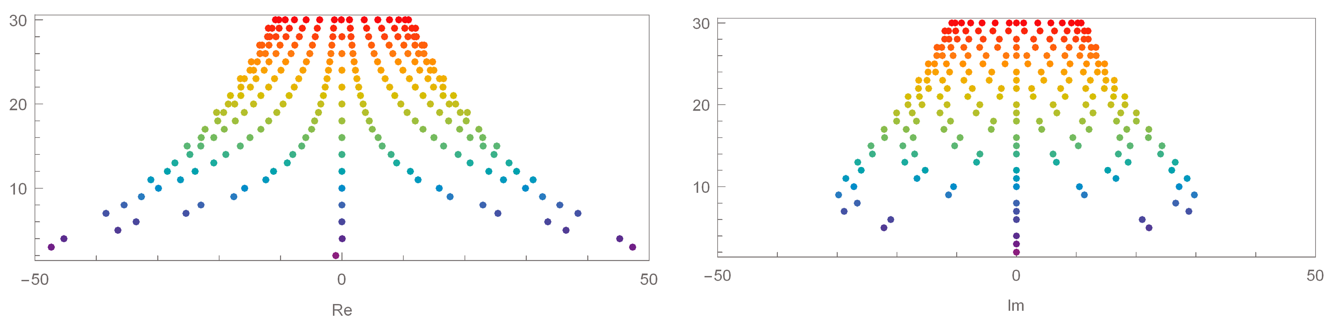
First, the structure of approximate roots in the $(p,q)$-cosine Bernoulli polynomials is illustrated in Figure 1 when $y=5$, $q=0.9$, and the value of p changes. Figure 1 reveals the pattern of the roots in the $(p,q)$-cosine Bernoulli polynomials when $p=0.5$. In addition, the approximate roots appear when n changes from 1 to 30. The red points become closer together when n is 30 and n becomes smaller as illustrated by the blue points. Based on the graphs with real and imaginary axes, the $(p,q)$-cosine Bernoulli polynomials are symmetric.

Here, we aim to confirm that changes in the value of the $(p,q)$-cosine Bernoulli polynomials changes the structure of the approximate roots as the value changes. The structure of the approximate roots in polynomials when $p=1$ and q changes, can be found in the q-cosine Bernoulli polynomials (see [11]).

Figure 2 below illustrates the stacking structure of the approximate roots of the $(p,q)$-cosine Bernoulli polynomials fixed at $p=0.1,q=0.5$ and $y=5$ when $1\le n\le 30$. Compared with Figure 1, Figure 2 displays a wider distribution of the approximate roots. The range of the left picture in Figure 1 is $-15<\mathrm{Re}x<15$ and the range of the left picture in Figure 2 is $-50<\mathrm{Re}x<50$. The structure of the approximate roots of $p=0.1$ when $n=30$ is wider on the real axis compared to when $p=0.5$. The right-hand graphs in Figure 1 and Figure 2 also reveal the same distribution. In addition, as n increases, the structure of the approximate roots appears symmetric.

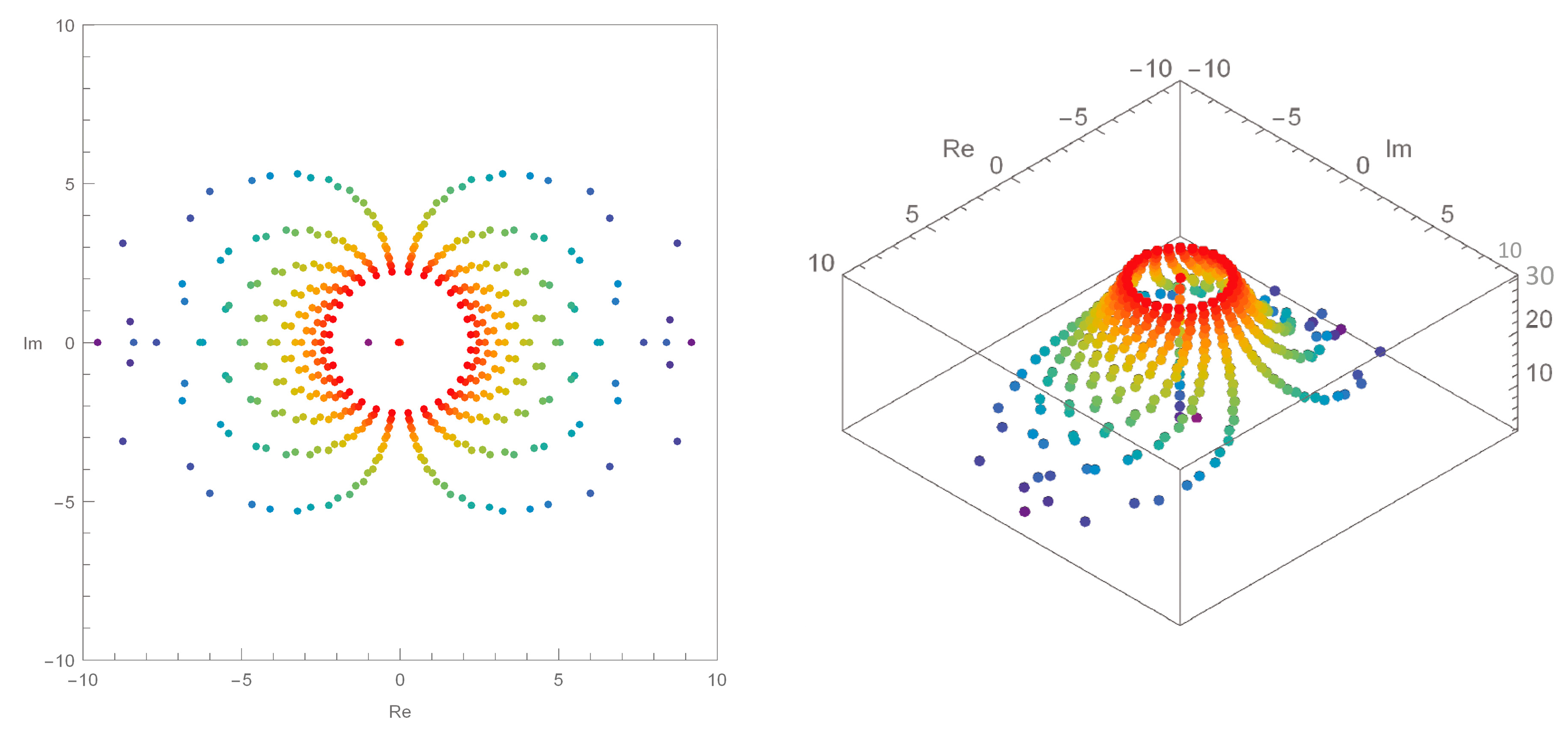
Next, we examine the stacking structure of the approximate roots in the $(p,q)$-sine Bernoulli polynomials. The conditions are confirmed by equating them to the conditions of the $(p,q)$-cosine Bernoulli polynomials. The stacking structure of the approximate roots of the $(p,q)$-sine Bernoulli polynomials when $p=0.5,q=0.9$, and $y=5$ can be checked in Figure 3. At $1\le n\le 30$, the distribution range of the approximate roots appears wider in the values on the real axis than in the imaginary axis, as shown in the left picture in Figure 3. Figure 3 reveals that, as the value of n becomes larger, the approximate roots become more symmetric, and the approximate form approaches a circular shape, including the origin.

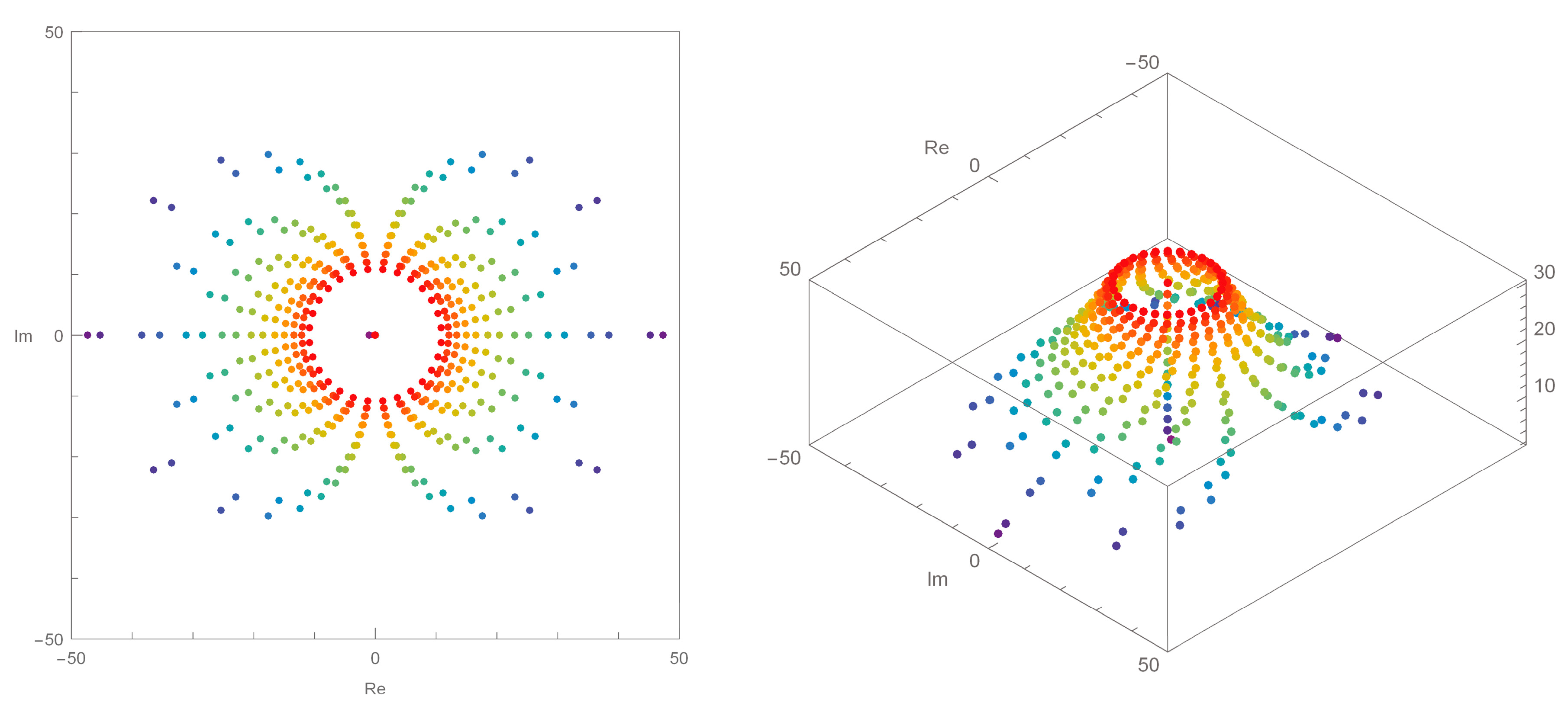
When we change the value of p, the structure of the approximate roots of the $(p,q)$-sine Bernoulli polynomials when $p=0.1$ under the same conditions as in Figure 3 is presented in Figure 4. In comparison with Figure 3, the area of the real and the imaginary axes in Figure 4 is greater, and the approximate roots have a wider distribution than observed in Figure 3. This property is common in the approximate roots of the $(p,q)$-cosine and $(p,q)$-sine Bernoulli polynomials. This indicates that, as the value of p decreases, the approximate roots of the $(p,q)$-cosine and $(p,q)$-sine Bernoulli polynomials spread wider. In addition, as displayed in Figure 4, the structure of the approximate roots of the $(p,q)$-sine Bernoulli polynomials is symmetric as the value of n increases.

5. Conclusions and Future Directions

In this paper, we explained about the $(p,q)$-cosine and $(p,q)$-sine Bernoulli polynomials, their basic properties, and various symmetric properties. Based on the above contents, we identified the structures of the approximate roots of the $(p,q)$-cosine and $(p,q)$-sine Bernoulli polynomials. As a result, we observed that the above polynomials obtain a structure of approximate roots, which has certain patterns and has a symmetric property under the given circumstances.

Further study is needed regarding whether the structure of approximate roots for the $(p,q)$-cosine and $(p,q)$-sine Bernoulli polynomials have symmetric properties under different circumstances. Furthermore, we think researching theories related to this topic is important to mathematicians.

References

- Brodimas, G.; Jannussis, A.; Mignani, R. Two-Parameter Quantum Groups; Universita di Roma: Piazzale Aldo Moro, Roma, Italy, 1991; p. 820, View in KEK Scanned Document. [Google Scholar]
- Chakrabarti, R.; Jagannathan, R. A (p, q)-oscillator realization of two-parameter quantum algebras. J. Phys. A Math. Gen. 1991, 24, L711–L718. [Google Scholar] [CrossRef]
- Burban, I.M.; Klimyk, A.U. (p, q)-differentiation, (p, q)-integration and (p, q)-hypergeometric functions related to quantum groups. Integral Transform. Spec. Funct. 1994, 2, 15–36. [Google Scholar] [CrossRef]
- Jagannathan, R. (P, Q)-special functions, special functions and differential equations. In Proceedings of a Workshop; The Institute of Mathematical Science: Matras, India, 1997; pp. 13–24. [Google Scholar]
- Jagannathan, R.; Rao, K.S. Two-parameter quatum algebras, twin-basic numbers, and associated generalized hypergeometric series. In Proceedings of the Lnternational Conference on Number Theory and Mathematical Physics, Srinivasa Ramanujan Centre, Kumbakonam, India, 20–21 December 2005. [Google Scholar]
- Corcino, R.B. On P,Q-Binomials coefficients. Electron. J. Combin. Number Theory 2008, 8, 1–16. [Google Scholar]
- Sadjang, P.N. On the (p, q)-Gamma and the (p, q)-Beta functions. arXiv 2015, arXiv:1506.07394v1. [Google Scholar]
- Kupershmidt, B.A. Reflection Symmetries of q-Bernoulli Polynomials. J. Nonlinear Math. Phys. 2005, 12, 412–422. [Google Scholar] [CrossRef]
- Kim, T.; Ryoo, C.S. Some identities for Euler and Bernoulli polynomials and their zeros. Axioms 2018, 7, 56. [Google Scholar] [CrossRef] [Green Version]
- Kim, T. q-generalized Euler numbers and polynomials. Russ. J. Math. Phys. 2006, 13, 293–298. [Google Scholar] [CrossRef] [Green Version]
- Kang, J.Y.; Ryoo, C.S. Various structures of the roots and explicit properties of q-cosine Bernoulli Polynomials and q-sine Bernoulli Polynomials. Mathematics 2020, 8, 463. [Google Scholar] [CrossRef] [Green Version]
- Ryoo, C.S. A note on the zeros of the q-Bernoulli polynomials. J. Appl. Math. Inform. 2010, 28, 805–811. [Google Scholar]
- Duran, U.; Acikgoz, M.; Araci, S. On some polynomials derived from (p, q)-calculus. J. Comput. Theor. Nanosci. 2016, 13, 7903–7908. [Google Scholar] [CrossRef]
- Duran, U.; Acikgoz, M.; Araci, S. On (p, q)-Bernoulli, (p, q)-Euler and (p, q)-Genocchi polynomials. J. Comput. Theor. Nanosci. 2016, 13, 7833–7846. [Google Scholar] [CrossRef]
- Acar, T.; Aral, A.; Mohiuddine, S.A. On Kantorovich modifivation of (p, q)-Baskakov operators. J. Inequal. Appl. 2016, 98, 1–14. [Google Scholar]
- Arik, M.; Demircan, E.; Turgut, T.; Ekinci, L.; Mungan, M. Fibonacci Oscillators. Z. Phys. C-Part. Fiels 1992, 55, 89–95. [Google Scholar] [CrossRef]
- Duran, U.; Acikgoz, M.; Araci, S. A study on some new results arising from (p, q)-calculus. TWMS J. Pure Appl. Math. 2020, 11, 57–71. [Google Scholar]
- Jackson, H.F. On q-definite integrals. Q. J. Pure Appl. Math. 1910, 41, 193–203. [Google Scholar]
- lSadjang, P.N. On the fundamental theorem of (p, q)-calculus and some (p, q)-Taylor formulas. arXiv 2013, arXiv:1309.3934. [Google Scholar]
- Wachs, M.; White, D. (p, q)-Stirling numbers and set partition statistics. J. Combin. Theorey Ser. A 1991, 56, 27–46. [Google Scholar] [CrossRef] [Green Version]
Figure 1.
Stacking structure of approximate roots in the -cosine Bernoulli polynomials when , and .
Figure 2.
Figure 3.
Stacking structure of approximate roots in the -sine Bernoulli polynomials when , and in 3D.
Figure 4.
© 2020 by the authors. Licensee MDPI, Basel, Switzerland. This article is an open access article distributed under the terms and conditions of the Creative Commons Attribution (CC BY) license (http://creativecommons.org/licenses/by/4.0/).
Share and Cite
MDPI and ACS Style
Ryoo, C.S.; Kang, J.Y. Structure of Approximate Roots Based on Symmetric Properties of (p, q)-Cosine and (p, q)-Sine Bernoulli Polynomials. Symmetry 2020, 12, 885. https://doi.org/10.3390/sym12060885
AMA Style
Ryoo CS, Kang JY. Structure of Approximate Roots Based on Symmetric Properties of (p, q)-Cosine and (p, q)-Sine Bernoulli Polynomials. Symmetry. 2020; 12(6):885. https://doi.org/10.3390/sym12060885
Chicago/Turabian StyleRyoo, Cheon Seoung, and Jung Yoog Kang. 2020. "Structure of Approximate Roots Based on Symmetric Properties of (p, q)-Cosine and (p, q)-Sine Bernoulli Polynomials" Symmetry 12, no. 6: 885. https://doi.org/10.3390/sym12060885
Note that from the first issue of 2016, this journal uses article numbers instead of page numbers. See further details here.