New Fixed Point Results via (θ,ψ)R-Weak Contractions with an Application
by
 , and
, and
Mohammad Imdad
1,†, 
Based Ali
1,†,
Waleed M. Alfaqih
2,*,†,
Salvatore Sessa
3,*,† and
Abdullah Aldurayhim
4,† 1
Department of Mathematics, Aligarh Muslim University, Aligarh 202002, India
2
Department of Mathematics, Hajjah University, Hajjah 1729, Yemen
3
Dipartimento di Architettura, Università degli Studi di Napoli Federico II, Via Toledo 402, 80134 Napoli, Italy
4
Department of Mathematics, Prince Sattam Bin Abdulaziz University, Alkharj 11911, Saudi Arabia
*
Authors to whom correspondence should be addressed.
†
These authors contributed equally to this work.
Symmetry 2020, 12(6), 887; https://doi.org/10.3390/sym12060887
Submission received: 2 May 2020
/
Revised: 25 May 2020
/
Accepted: 26 May 2020
/
Published: 30 May 2020
Abstract
:In this paper, inspired by Jleli and Samet (Journal of Inequalities and Applications 38 (2014) 1–8), we introduce two new classes of auxiliary functions and utilize the same to define -weak contractions. Utilizing -weak contractions, we prove some fixed point theorems in the setting of relational metric spaces. We employ some examples to substantiate the utility of our newly proven results. Finally, we apply one of our newly proven results to ensure the existence and uniqueness of the solution of a Volterra-type integral equation.
1. Introduction
Fixed point theory remains a very important and popular tool in pure, as well as applied mathematics, especially in the existence and uniqueness theories. It contains classical results to establish the existence and uniqueness theorems in ordinary differential equations, partial differential equations, integral equations, random differential equations, matrix equations, functional equations, iterated function systems, variational inequalities, etc. The Banach contraction principle [1] is one of the pivotal results of fixed point theory, which asserts that every contraction mapping defined on a complete metric space to itself always admits a unique fixed point. This principle is a very effective and popular tool for guaranteeing the existence and uniqueness of the solution of certain problems arising within and beyond mathematics. This principle has been generalized and extended in several directions. For this kind of work, one may recall Boyd and Wong [2], Matkowski [3], Ciric [4], Ran and Reurings [5], Jleli and Samet [6], and Imdad et al. [7], among others. As the Banach contraction principle and its extensions are existence and uniqueness results, they are very effectively utilized in several kinds of applications in the entire domain of mathematical and physical sciences, which also includes economics. One of the well-known extensions of the Banach contraction principle is due to Jleli and Samet [6], which is known as -contractions (or -contractions). In order to define -contractions, Jleli and Samet [6], in 2014, introduced a new class of auxiliary functions as given below.
Definition 1.
Let be a function satisfying the following conditions:
- θ is nondecreasing,
- for any iff ,
- there exists and satisfying ,
- θ is continuous.
Jleli and Samet [6] proved the following result:
Theorem 1.
[6] Let be a complete generalized metric space and . Assume that there exist θ satisfying , and such that:
Then, f has a unique fixed point.
The mapping f in Theorem 1 is called -contraction (or -contraction).
In 2015, Hussain et al. [8] extended Theorem 1 for some new contraction mappings in which the authors used the condition instead of . Imdad et al. [7] relaxed the condition and called such mappings weak -contractions.
On the other hand, there is yet another way to improve the Banach contraction principle utilizing various types of binary relations. In 2004, Ran and Reurings [5] proved a fixed point result in metric space equipped with a partial order relation, which was further generalized by Nieto and Rodríguez-López in [9,10]. In the same quest, in 2015, Alam and Imdad [11] generalized the Banach contraction to a complete relational metric space.
The study of this paper goes in four directions, which can be described as follows:
- to introduce the notion of -weak contraction;
- to prove our results in the setting of relational metric spaces;
- to adopt some examples substantiating the utility of our proven results;
- to utilize our newly proven results and establish an existence and uniqueness result for the solution of a Volterra-type integral equation.
2. Preliminaries
In this manuscript, the set of all fixed points of is denoted as For simplicity, sometimes we write instead of .
Our main results involve relation theoretic concepts. Therefore, we recall some preliminaries of the same.
Definition 2.
[12] Let E be a nonempty set. A subset of is said to be a binary relation on E. For with , we say that “a is related to b” or “a relates to b under ”. Sometimes, we write instead of . If , we say “a is not related to b” or “a does not relate to b under ”. If implies , then is called transitive.
In this paper, denotes a nonempty binary relation defined on a nonempty set E. For brevity, we only use “binary relation” instead of “nonempty binary relation”.
Definition 3.
[11]
- A binary relation on E is said to be f-closed if, for any ,
- A sequence is called -preserving if .
Definition 4.
A sequence is called an -preserving Cauchy sequence if it is a Cauchy sequence and .
Definition 5.
- is called d-self-closed if, for any -preserving sequence converging to a, there exists a subsequence with .
- is called -complete if every -preserving Cauchy sequence in E converges in E.
- A mapping is called -continuous at if for any -preserving sequence converging to a, we have . Moreover, f is -continuous on E if it is -continuous at each point of E.
We need the following lemma in the sequel.
Lemma 1.
[14] Let be a metric space and such that . If is not Cauchy, then there exist and two subsequences and of with such that:
3. Main Results
Firstly, we introduce the following two classes of auxiliary functions, which are relatively larger than the class of the auxiliary functions covered under Definition 1.
Definition 6.
Let Θ be the collection of all that satisfy the following conditions:
- for every sequence iff ,
- θ is lower semicontinuous.
The following examples of the functions belong to the class of :
Example 1.
,
Example 2.
,
Example 3.
,
Example 4.
.
Next, we introduce yet another class of auxiliary functions:
Definition 7.
Let Ψ be the collection of all that satisfy the following conditions:
- for every sequence iff ,
- ψ is right upper semicontinuous.
The following mappings belong to the class :
Example 5.
,
Example 6.
,
Example 7.
,
Example 8.
.
In what follows, we write .
Finally, we introduce the concept of -weak contractions as follows:
Definition 8.
Let be a metric space, a binary relation on E, and . Then, f is called a -weak contraction if there exist and with () such that:
with and .
Now, we state and prove our first main result as follows:
Theorem 2.
Let be a metric space endowed with a transitive binary relation and . Assume that:
- (i)
- E is -complete,
- (ii)
- there exists such that ,
- (iii)
- is f-closed,
- (iv)
- f is -weak contraction and
- (v)
- f is -continuous.
Then, f has a fixed point.
Proof.
In view of , there is such that . Consider the sequence of Picard iterates of f based at , i.e.,
If , for some , then , i.e., is a fixed point of f, and there is nothing to prove. Now, assume that for all . We claim that the sequence {} is -preserving. Due to Condition and (2), we have and ; hence, . Suppose , for some . As is f-closed, we have , i.e., . Hence, by mathematical induction, we conclude that is -preserving and , for all .
In view of the contraction condition (2), we have:
where :
as and whenever and .
If =, then,
a contradiction. Hence,
so that:
as . Finally, we have:
Now, letting , we obtain:
Making use of , we get:
Now, we proceed to prove that is Cauchy. Let on the contrary not be Cauchy. From Lemma 1, one can infer that there exist an and with such that:
tend to when .
As is transitive, so , for all . Furthermore, for sufficiently large , for all (as ). Therefore, we have:
so that:
wherein :
Observe that:
.
Now, as , and , so due to Lemma 1, we have:
On using (3), (4), and (5), we get:
a contradiction. Thus, is Cauchy. As is -preserving Cauchy in E, which is -complete, therefore, there is some such that:
As f is -continuous, we obtain:
i.e., as . Now, using the uniqueness of the limit, we have . Hence, f has a fixed point in E. This ends the proof. □
Next, we adopt the following example, which exhibits the utility of Theorem 2.
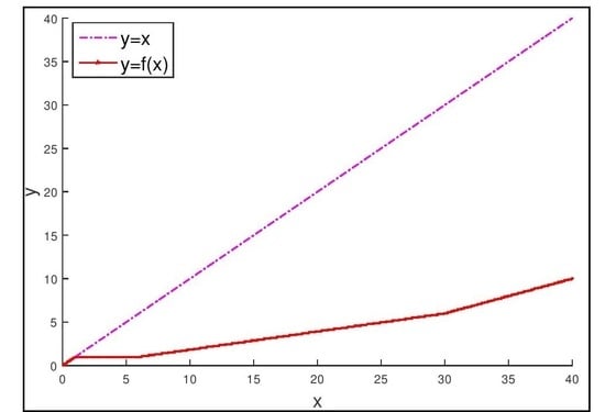
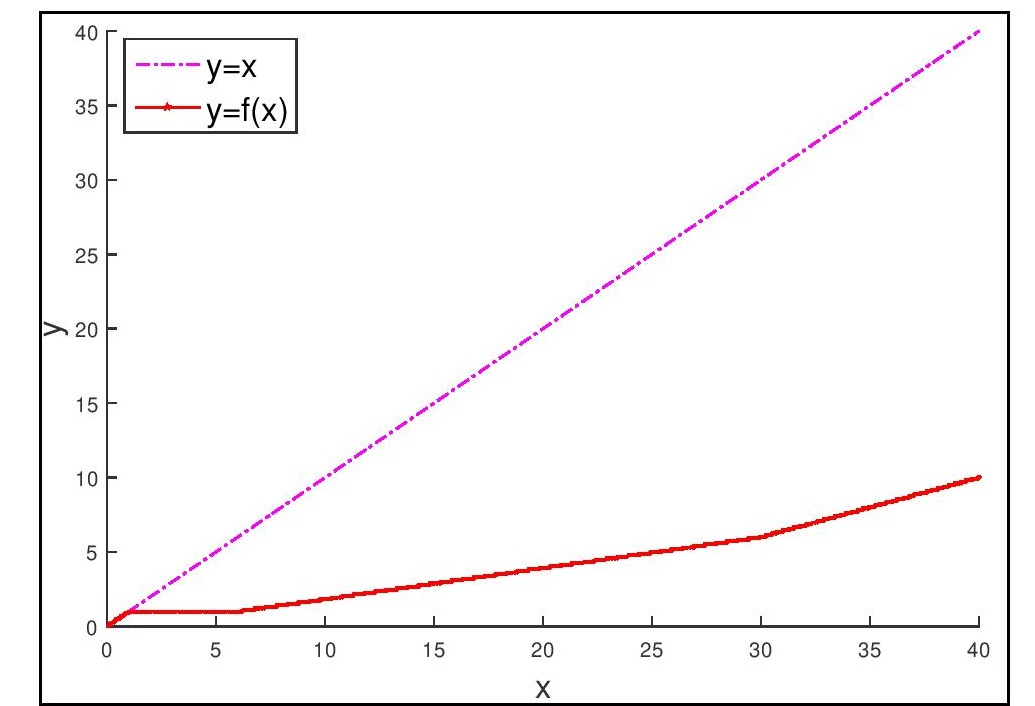
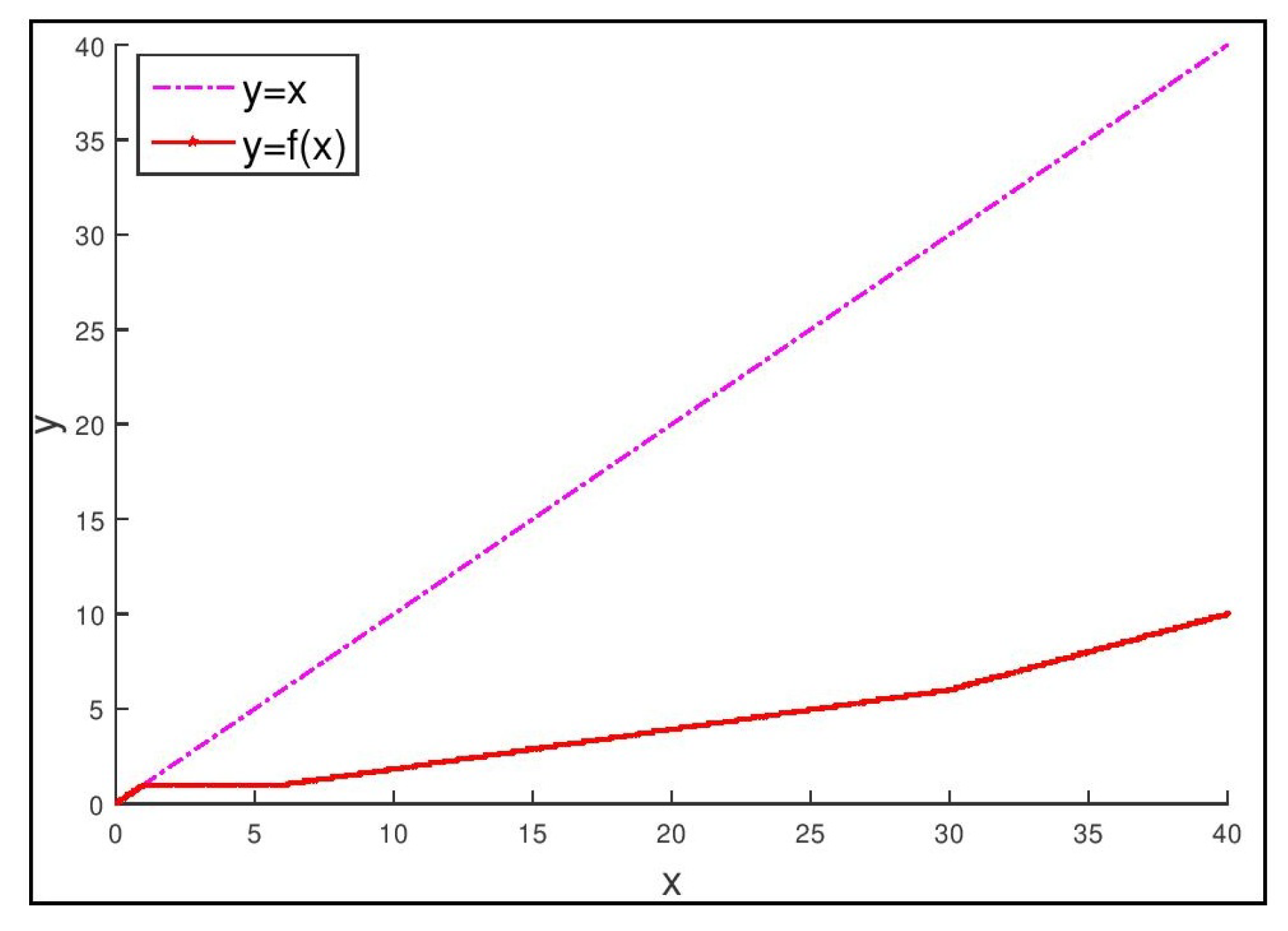
Example 9.
Let and d be the usual metric defined by , . Define as:
whose first few terms are 6, 30, 90, 210, and so on. Define a binary relation on E as:
Define f on E by:
The mapping f is continuous (see Figure 1).
To show that is f-closed, consider the following three different cases.
Case I: Let , then .
Case II: When , then or , i.e., .
Case III: When , then or and, hence, . Thus, is f-closed.
Now, to show that f is a -weak contraction mapping, we define as follows:
where are given by:
We have to show that there exists some such that:
We do not need to consider the cases as . Now, we distinguish the following four cases.
Case I: If and then ,
so that:
Case II: If and , then
so that:
Case III: If and , then :
so that:
Case IV: If and , then :
so that:
Therefore, in all four cases, we have:
Thus, the condition (6) is satisfied if we take . Therefore, we have furnished a such that , for all with , i.e., f is a -weak contraction mapping on X. Observe that the remaining assumptions of Theorem 2 are also fulfilled. Thus, f possesses a fixed point in E. Observe that f has infinitely many fixed points; in fact, (see Figure 1).
The pre-existing results in this direction, say the results of Jleli and Samet [6], Hussain et al. [8], and Imdad et al. [7], cannot be applied in this example as these results require the contraction condition to hold on the whole space. However, in this example, the contraction condition holds for those , which are related under the binary relation .
Now, we prove an analog of Theorem 2 using the d-self-closedness property.
Theorem 3.
The conclusion of Theorem 2 holds true if Assumption (v) is replaced by:
is d-self-closed.
Proof.
On the lines of the proof of Theorem 2, we can show that is an -preserving Cauchy sequence converging to . Our aim is to show that . Suppose on the contrary that . In view of the condition (), there exists a subsequence with , for all . Now, as and , for sufficiently large , we have , for all . Hence, we have (for all ):
where :
As:
and the sequence converges to a with , we have (for all ):
so that (for all ):
As is lower semicontinuous, , which gives rise to the following:
This is a contradiction. Hence, the assumption is wrong. Therefore, we must have , i.e., a is a fixed point of f. This completes the proof. □
Next, we prove the following corresponding uniqueness result.
Theorem 4.
If we assume in addition to the assumptions of Theorem 2 (or Theorem 3) that is complete or is -connected, then f has a unique fixed point in E.
Proof.
In view of Theorem 2 (or 3), we have is nonempty. Assume that is complete, and let be two different points in . Therefore, or , i.e., or . As and , we have . Hence, using the contraction condition , we get:
This is a contradiction as . Hence, our assumption that is wrong. Therefore, f has a unique fixed point in E.
Now, if is -connected and , then there exist in such that for all where . Now, as and for all from the earlier part of the theorem, we have , for all i. Therefore, , , the fixed point of f is unique. This concludes the proof. □
Now, to substantiate the utility of Theorems 3 and 4, we furnish the following example:
Example 10.
Let and d be the usual metric on E. Define on E as:
Then, is transitive. Now, define by:
We observe that the following holds:
- E is -complete, as for any -preserving Cauchy sequence in E, there exists such that , or , , i.e., converges to zero or one;
- and ;
- is f-closed;
Now, we show that f is a -weak contraction. Take as the following:
where are given by:
We have to show that there exists such that:
Observe that implies that . Therefore, we consider only the two cases and .
Case I: Let . Then:
Observe that,
Case II: If , then:
As:
Therefore, for , we have:
or:
for all with and . Hence, the Condition is satisfied.
Next, in order to verify , observe that for any -preserving sequence converging to some , there is some such that either , for all or , for all . Hence, is a subsequence of such that for each .
Therefore, all the assumptions of Theorem 3 are satisfied. Hence, f has a fixed point in E. We can see that zero is the fixed point of f. Furthermore, , which is complete as . Thus, Theorem 4 ensures the uniqueness of the fixed point of f.
4. Applications
In this section, we apply Theorem 4 to ensure the existence and uniqueness of the solution for the following integral equation:
where G is a continuous function from to [0, 1] and g is a continuous function from [0, 1] to [0, 1].
Consider the Banach space of all continuous functions equipped with the norm:
Define a metric d on E by:
Then, is a complete metric space.
Now, we state and prove our first result in this section as follows:
Theorem 5.
If G is nondecreasing in the third variable and there exists such that:
for all such that , then the existence of a lower solution of the integral Equation (8) ensures the existence of a unique solution of the same.
Proof.
Define a self-mapping by:
Define on E by:
For any , we have:
Therefore, is f-closed. In the hypotheses, we assumed the existence of a lower solution of (8), i.e., there is some such that the following holds:
Therefore, is such that for each . Hence, . Now, for any such that , we have:
Consider ; then, f becomes a -weak contraction. Now, for any -preserving sequence in E converging to , we have:
Thus, for all . Therefore, is d-self-closed in E. Hence, using Theorem 2, we conclude that f has a fixed point, i.e., there is some such that:
Now, for any and . Furthermore, , i.e., and . Therefore, is connected. Hence, Theorem 4 ensures the uniqueness of the solution of the integral Equation (8). This accomplishes the proof. □
Next, we provide the following theorem in the presence of an upper solution.
Theorem 6.
If G is nondecreasing in the third variable and such that:
for all such that , then the existence of an upper solution of the integral Equation (8) ensures the existence of a unique solution of the same.
Proof.
In this case, we define the binary relation as follows:
Now, following the same steps as Theorem 5 one can see that all the hypotheses of Theorem 4 hold true. Therefore, the existence and uniqueness of the solution of the integral equation (8) are ensured (due to Theorem 4). □
Author Contributions
All the authors contributed equally and significantly in writing this article. All authors read and approved the final manuscript.
Funding
This research received no external funding.
Acknowledgments
All the authors are grateful to the anonymous referees for their excellent suggestions, which greatly improved the presentation of the paper.
Conflicts of Interest
The authors declare no conflict of interest.
References
- Banach, S. Sur les opérations dans les ensembles abstraits et leur application aux équations intégrales. Fund. Math 1922, 1, 133–181. [Google Scholar] [CrossRef]
- Boyd, D.W.; Wong, J.S. On nonlinear contractions. Proc. Am. Math. Soc. 1969, 2, 458–464. [Google Scholar] [CrossRef]
- Matkowski, J. Integrable Solutions of Functional Equations; Instytut Matematyczny Polskiej Akademi Nauk: Warszawa, Poland, 1975. [Google Scholar]
- Ćirić, L.B. Generalized contractions and fixed-point theorems. Publ. Inst. Math. (Beograd) (NS) 1971, 26, 19–26. [Google Scholar]
- Ran, A.C.; Reurings, M.C. A fixed point theorem in partially ordered sets and some applications to matrix equations. Proc. Am. Math. Soc. 2004, 132, 1435–1443. [Google Scholar] [CrossRef]
- Jleli, M.; Samet, B. A new generalization of the banach contraction principle. J. Inequalities Appl. 2014, 38, 1–8. [Google Scholar] [CrossRef] [Green Version]
- Imdad, M.; Alfaqih, W.M.; Khan, I.A. Weak θ-contractions and some fixed point results with applications to fractal theory. 2018; Submitted. [Google Scholar]
- Hussain, N.; Parvaneh, V.; Samet, B.; Vetro, C. Some fixed point theorems for generalized contractive mappings in complete metric spaces. Fixed Point Theory Appl. 2015, 185, 1–17. [Google Scholar] [CrossRef] [Green Version]
- Nieto, J.J.; Rodríguez-López, R. Contractive mapping theorems in partially ordered sets and applications to ordinary differential equations. Order 2005, 3, 223–239. [Google Scholar] [CrossRef]
- Nieto, J.J.; Rodríguez-López, R. Existence and uniqueness of fixed point in partially ordered sets and applications to ordinary differential equations. Acta Math. Sin. Engl. Ser. 2007, 12, 2205–2212. [Google Scholar] [CrossRef]
- Alam, A.; Imdad, M. Relation-theoretic contraction principle. J. Fixed Point Theory Appl. 2015, 4, 693–702. [Google Scholar] [CrossRef]
- Lipschutz, S. Schaum’s Outline of Theory and Problems of Set Theory and Related Topics; Tata McGraw-Hill: New Delhi, India, 1976. [Google Scholar]
- Alam, A.; Imdad, M. Relation-theoretic metrical coincidence theorems. Filomat 2017, 14, 4421–4439. [Google Scholar] [CrossRef] [Green Version]
- Berzig, M.; Karapınar, E.; Roldán-López-de Hierro, A.-F. Discussion on generalized-(αψ, β)-contractive mappings via generalized altering distance function and related fixed point theorems. In Abstract and Applied Analysis; Hindawi Publishing Corporation: New York, NY, USA, 2014; Volume 2014. [Google Scholar]
Figure 1.
Graph of and in Example 9.

© 2020 by the authors. Licensee MDPI, Basel, Switzerland. This article is an open access article distributed under the terms and conditions of the Creative Commons Attribution (CC BY) license (http://creativecommons.org/licenses/by/4.0/).
Share and Cite
MDPI and ACS Style
Imdad, M.; Ali, B.; Alfaqih, W.M.; Sessa, S.; Aldurayhim, A. New Fixed Point Results via (θ,ψ)R-Weak Contractions with an Application. Symmetry 2020, 12, 887. https://doi.org/10.3390/sym12060887
AMA Style
Imdad M, Ali B, Alfaqih WM, Sessa S, Aldurayhim A. New Fixed Point Results via (θ,ψ)R-Weak Contractions with an Application. Symmetry. 2020; 12(6):887. https://doi.org/10.3390/sym12060887
Chicago/Turabian StyleImdad, Mohammad, Based Ali, Waleed M. Alfaqih, Salvatore Sessa, and Abdullah Aldurayhim. 2020. "New Fixed Point Results via (θ,ψ)R-Weak Contractions with an Application" Symmetry 12, no. 6: 887. https://doi.org/10.3390/sym12060887
Note that from the first issue of 2016, this journal uses article numbers instead of page numbers. See further details here.