Article

3D Characterization of a Coastal Freshwater Aquifer in SE Malta (Mediterranean Sea) by Time-Domain Electromagnetics

1
Department of Geology and Geophysics, Texas A&M University, College Station, TX 77843, USA
2
Marine Geology and Seafloor Surveying, Department of Geosciences, University of Malta, MSD 2080 Msida, Malta
3
GEOMAR—Helmholtz Centre for Ocean Research Kiel, Wischhofstraße 1-3, D-24148 Kiel, Germany
*
Author to whom correspondence should be addressed.
Water 2020, 12(6), 1566; https://doi.org/10.3390/w12061566
Submission received: 27 March 2020 / Revised: 21 May 2020 / Accepted: 27 May 2020 / Published: 30 May 2020
(This article belongs to the Special Issue Applied Geophysics in Hydrogeological Practice)

Abstract

:
Electromagnetic (EM) geophysical methods are well equipped to distinguish electrical resistivity contrasts between freshwater-saturated and seawater-saturated formations. Beneath the semi-arid, rapidly urbanizing island of Malta, offshore groundwater is an important potential resource but it is not known whether the regional mean sea-level aquifer (MSLA) extends offshore. To address this uncertainty, land-based alongshore and across-shore time-domain electromagnetic (TDEM) responses were acquired with the G-TEM instrument (Geonics Ltd., Mississauga, ON, Canada) and used to map the onshore structure of the aquifer. 1-D inversion results suggest that the onshore freshwater aquifer resides at 4–24 m depth, underlain by seawater-saturated formations. The freshwater aquifer thickens with distance from the coastline. We present 2D and 3D electromagnetic forward modeling based on finite-element (FE) analysis to further constrain the subsurface geometry of the onshore freshwater body. We interpret the high resistivity zones that as brackish water-saturated bodies are associated with the mean sea-level aquifer. Generally, time-domain electromagnetic (TDEM) results provide valuable onshore hydrogeological information, which can be augmented with marine and coastal transition-zone measurements to assess potential hydraulic continuity of terrestrial aquifers extending offshore.

1. Introduction

Groundwater resources in many coastal regions worldwide are currently under stress because of increasing population, agricultural demands, tourism and economic growth. Fresh groundwater in coastal regions may be a resource that can help to mitigate the water scarcity experienced by coastal communities [1]. However, several first-order questions need to be addressed before the fresh groundwater can be used sustainably. There is a lack of understanding regarding the location, nature, and geometry of coastal aquifer systems and their offshore connectivity. Large-scale desalination of seawater is a technologically viable solution, but there are important energy and environmental impacts that must be considered [2]. Terrestrial time-domain electromagnetic (TDEM) methods of geophysical exploration employing a loop or grounded dipole source can be used to explore the onshore component of coastal aquifers that may extend offshore. TDEM methods are useful because they have good depth penetration in saline environments compared to other geophysical techniques, such as ground-penetrating radar (GPR) and electrical resistivity tomography (ERT). TDEM methods are sensitive to electrical resistivity which, in turn, is diagnostic of important aquifer parameters such as porosity, water saturation and salinity [3]. Transient electromagnetic (EM) methods respond to the interaction between an applied time-varying magnetic flux and the geoelectrical structure beneath the transmitter.
In order to interpret transient electromagnetic responses, the key physical mechanism is the induction process governed by Faraday’s law, which is equivalent to diffusion into a conducting medium of an image of the transmitter (TX) loop current. A fundamental overview of the physical principles underlying the EM geophysical method is given elsewhere [4,5], and there are many reviews related to near-surface applications of EM techniques, e.g., [6,7]. The TDEM method has been widely used for groundwater studies [8,9,10,11,12,13,14], including coastal aquifer characterization. The EM methods distinguish electrical conductivity contrasts between freshwater-saturated or brackish-water saturated formations (resistivity ~10–100 Ω m , or more) and seawater-saturated formations (resistivity ~1–10 Ω m ). A hydraulic connection implies a continuous hydraulic pathway beneath the coastal zone, such that an offshore aquifer could be recharged by its onshore counterpart, or depleted by pumping of its onshore counterpart. Terrestrial EM geophysical surveys can provide valuable information about the existence of such connections. This knowledge is important if we are to ensure the long-term sustainability of groundwater resources and it can serve as a valuable constraint for hydrogeological modeling studies. Onshore-offshore connectivity also has implications for possible onshore land subsidence due to offshore drilling and extraction [15,16]. It should also be noted that the electromagnetic method remains largely undeveloped for data acquisition in the important coastal shallow-water transition zone.
This study is part of a multi-disciplinary project that aims to investigate potential onshore-offshore groundwater aquifer connections based on terrestrial and offshore TDEM geophysical data from SE Malta (Mediterranean Sea). Here we utilize 2D and 3D electromagnetic forward modeling based on finite-element (FE) analysis to constrain the 3D geometry of the onshore freshwater body, in this case, the mean sea-level aquifer in SE Malta. To accomplish this objective, TDEM responses were acquired with the Geonics G-TEM instrument. The analysis of the TDEM data generated geoelectrical models that are used to better understand the variable coastal hydrogeology along a short segment of the Maltese coastline. This helps to characterize the potential groundwater resources of the semi-arid, rapidly urbanizing island of Malta. Future work, currently in the planning stages, will involve conducting additional EM measurements both offshore and within the coastal transition zone.

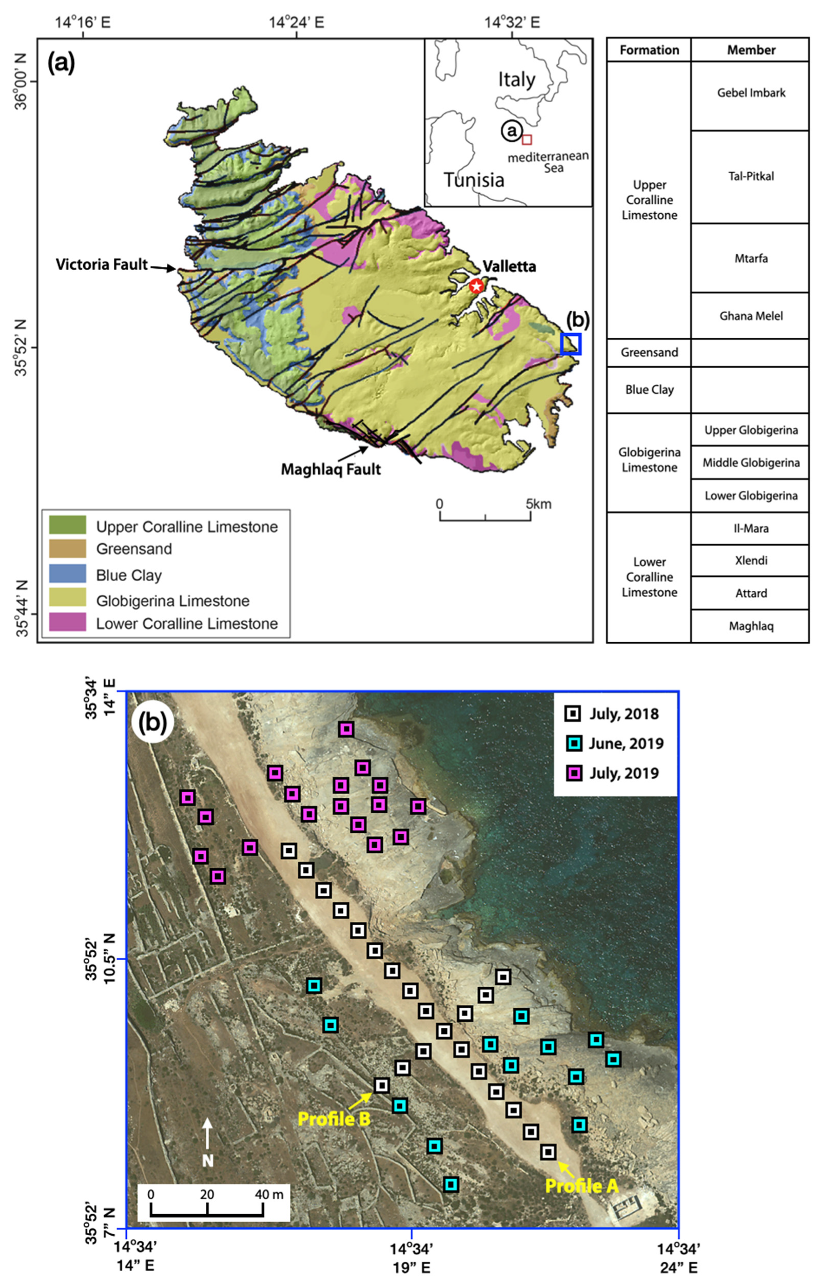
2. Characterization of Mean Sea-Level Aquifer and Study Area

The Maltese Islands, comprising of Malta, Gozo and Comino, are composed of marine sedimentary rocks deposited between the Late Oligocene and Late Miocene epochs [17]. The five sedimentary formations outcropping across the Maltese Islands include, from top to bottom: Upper Coralline Limestone (162 m), Greensand (11 m), Blue Clay (75 m), Globigerina Limestone (207 m), and Lower Coralline Limestone (up to 1 km, of which the top ~140 m is exposed) (numbers in brackets denote maximum thickness) (see Figure 1a) [18,19]. This succession contains a range of lithologies and facies, but overall it is dominated by marine carbonates of shallow water origin. The rock formations exhibit a gentle regional flexure and normal faulting is widespread [20]. The older (Early Miocene) and most widespread system of faults is oriented SW–NE and includes the Great Fault or Victoria Fault, which is ~11 km long and traverses the entire width of the island. A younger system of faults (Late Miocene-Early Pliocene) is present along the southern coastline and often cross-cuts pre-existing faults. The longest of the younger faults is the NW–SE striking Maghlaq Fault. The climate of Malta is semi-arid Mediterranean characterized by a hot, dry summer and a mild, humid winter. The mean annual precipitation is 550 mm, which mainly falls between September and April [21,22].
The Maltese Islands obtain ~55% of their potable water supply from groundwater, while the rest comes from seawater desalination [22]. Aquifers are the primary source of portable water as there is no appreciable surface water streamflow. The mean sea-level groundwater body lies within the pores and fissures of Lower Coralline Limestone (LCL) in the interval where the formation sub-crops at sea-level south of the Victoria fault [23]. The LCL formation is predominantly composed of an algal fossiliferous limestone with sparse corals. The rocks exhibit moderate, irregular or channel-like permeability [24]. The primary porosity of LCL ranges between 7 and 20%, whereas its intrinsic permeability is low (10−7–10−9 m/s). Effective porosity and secondary permeability, both of which are dependent on fissures and weathering, have values of 10–15% and 10−6 m/s [23,25]. The mean sea-level groundwater body is in lateral and vertical contact with seawater. A body of fresh water in the form of a ‘lens’ floats on saline water due to its lower density [26,27]. The thicker part of the lens is situated in the central part of Malta, with its height decreasing towards the coastline. The mean-sea level groundwater is not at rest, but flows horizontally outward from the thickest part. The aquifer is recharged by the infiltration of rainwater in every winter, and groundwater is either discharged offshore at the coastline or else removed by abstraction (pumpage) for agricultural purposes. The mean sea-level aquifer (MSLA) has a mean thickness of 67.5 m and covers an area of >200 km2 [28]. This water is mainly abstracted for potable supply and agricultural use. A number of discontinuous perched aquifers with a limited saturated thickness occur north of the Great Fault in the Upper Coralline Limestone above the impermeable Blue Clay, and they are exclusively used for agricultural purposes.
The study site is situated on the SE coast of the island of Malta ~6 km SE of Valletta, the capital city. The elevation of the study site is ~10 m above the sea surface (see Figure 1a). The rocks exposed at the study site consist of the lower member of the Globigerina Limestone formation, which overlies the upper members of the LCL formation. There is a geological well at 3.5 km west of the study site that shows 35 m of Lower Globigerina above 34 m of Lower Coralline and the elevation of the well is 35 m [29]. There is another well drilled for hydrological purposes, located 2.5 km west of the study site, where the top of the water table is 1 m above sea level [26].

3. Methods

This study utilizes the near-surface TDEM geophysical method to determine the geometry and characteristics of the onshore MSLA along the coast at the survey site in SE Malta. The TDEM measurements were carried out using the Geonics G-TEM system consisting of a portable battery-operated transmitter-receiver (TX-RX) console, a TX antenna deployed as 4 turns of a 10 × 10 m square loop of wire laid on the ground, a 0.6 m diameter RX rigid coil with pre-amplifier, and the supporting cables. In field operations, the equipment was deployed as shown in Figure 2. In this study, all soundings were acquired in the 20 time-gate mode, corresponding to investigation depths of 60–100 m. The 30-gate mode with longer acquisition time allowing for deeper exploration was not used. The depth of investigation also depends on the TX power, which is a product of the loop size, current, and its number of turns, in addition to the subsurface conductivity and the RX sensitivity [30].
The operating principle of TDEM is based on the EM induction process. An abrupt shut-off of a steady value of TX current in the wire loop, according to Faraday’s law, generates an impulsive electromotive force (emf) that drives eddy current flow in the conductive earth. After the shut-off, the emf vanishes and the eddy currents start to decay. A weak secondary magnetic field is produced in proportion to the deceasing amplitude of the eddy currents. The multi-turn receiver coil located at the ground surface measures the time rate of change of the decaying secondary vertical magnetic field, the decay rate being diagnostic of the subsurface electrical resistivity.

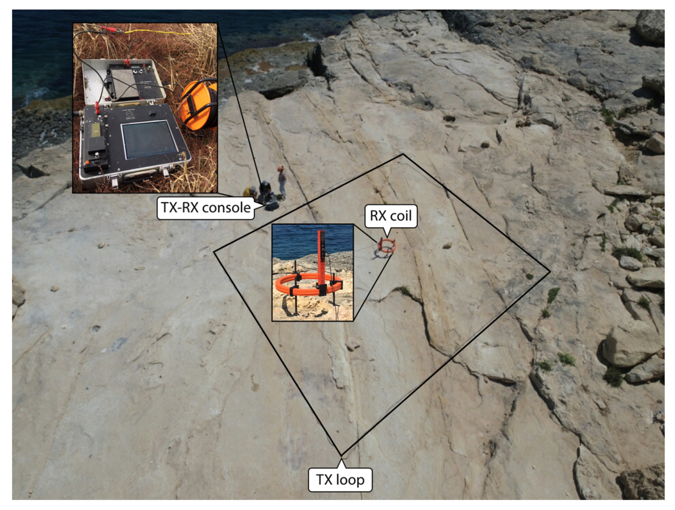
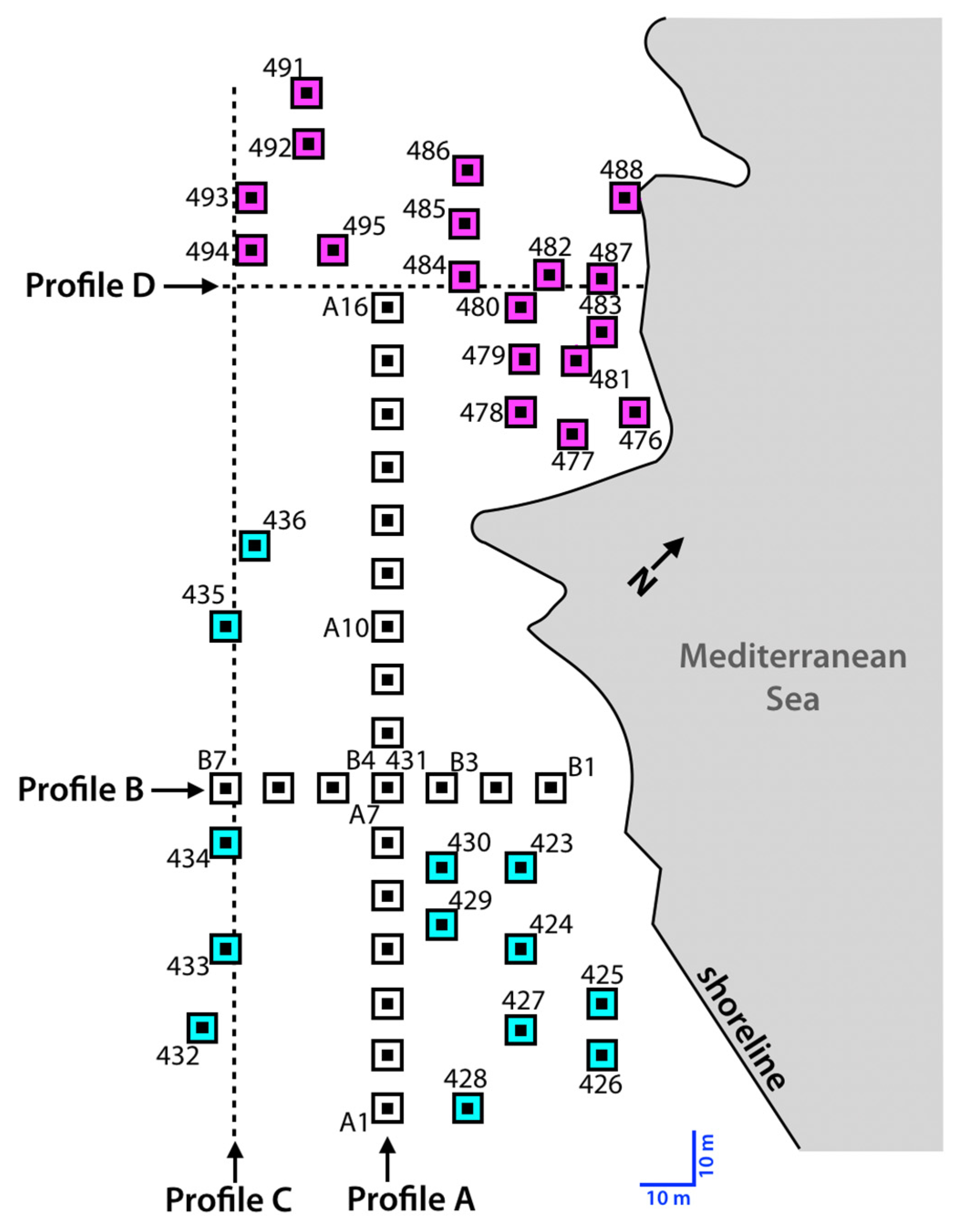
3.1. Data Acquisition
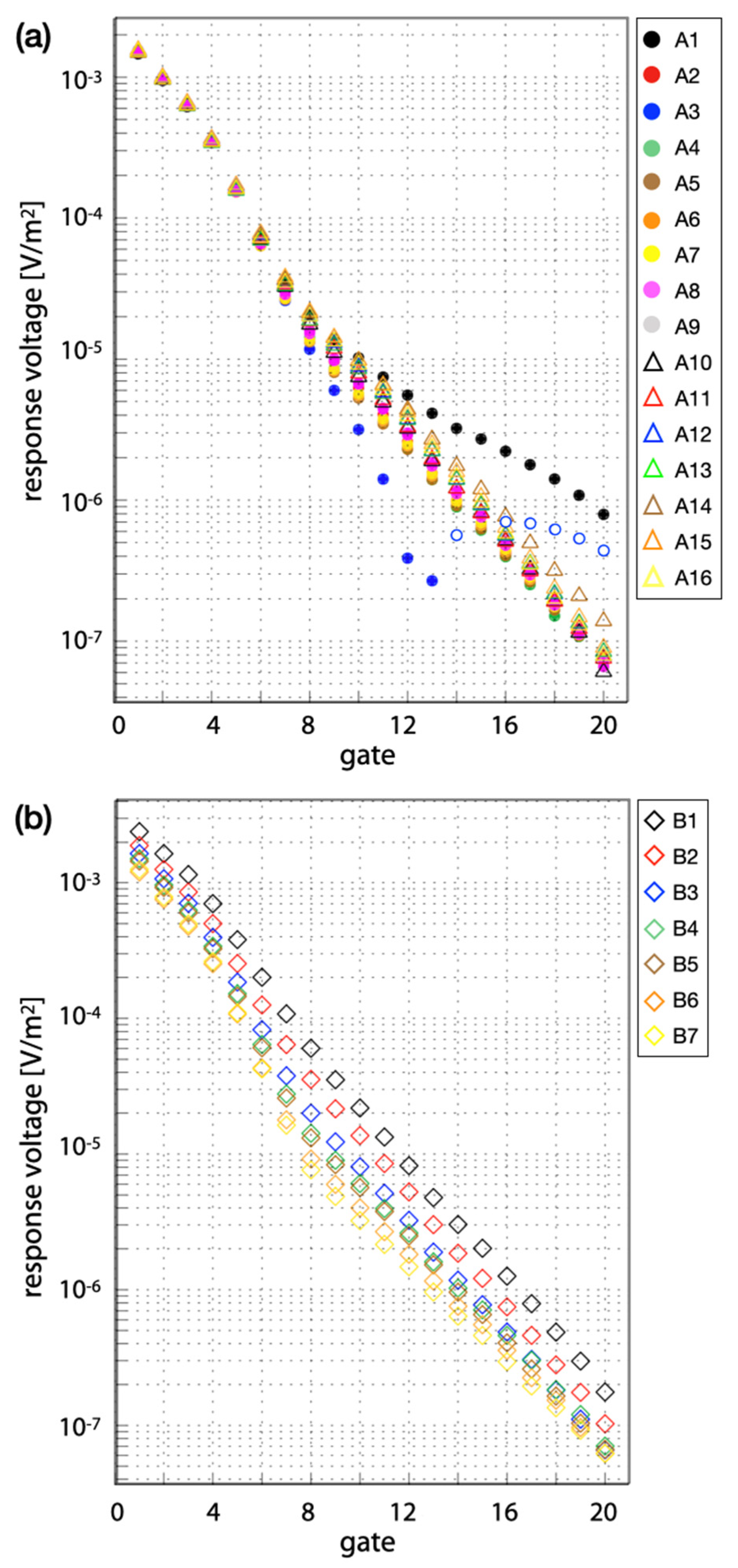
The geophysical survey procedure was as follows. At each sounding location, the wire loop was laid out on the ground. Then the RX coil with its pre-amplifier was set up in the center of the wire loop, to achieve a central-loop sounding. The portable TX-RX console was set up immediately outside the TX loop for convenience. A ramp-off current was passed through the wire loop using the signal generator in the TX console. The resultant signal received by the RX coil was recorded by the RX console, averaged over several thousand repetitions to improve signal-to-noise ratio. The overall time to acquire each sounding response was ~5 min. Then the TX loop and RX coil were picked up, along with the TX-RX console, and moved forward to the next sounding location. The center of the RX coil represents the location of each sounding, the latter recorded by handheld GPS. The operating frequency, i.e., the repetition rate of the TX on/off cycle, is in the kHz range (i.e., well outside the main power supply at 50 Hz and cell phones at ~1 GHz.) The TDEM method is non-invasive, and no significant environmental disturbance is made to natural flora, wildlife, or agriculture.
The two orthogonal transects acquired in SE Malta comprising a total of 23 TDEM central-loop soundings in July 2018 are marked as black-and-white symbols in Figure 1b. Profile A is oriented from SE to NW along the shoreline with a total length of 150 m, while profile B is aligned from NE to SW with a length of 60 m (Figure 3). The two profiles cross each other at stations A7 and B4, respectively. An additional dataset of 31 soundings (cyan and purple symbols in Figure 1b; see also Figure 3) was added to this area from a second field survey conducted during June and July 2019. One of the 2019 soundings (station 431) was performed at the crossing point of the two previous transects (A, B) to check signal repeatability. The 2019 survey was performed in order to expand the coverage of the survey from the previous year. The rationale for adding more soundings is that the denser spatial distribution of data enables us to better construct a fully 3D geoelectrical model.

3.2. Data Analysis

3.2.1. D Inversion

The 1D inversion of G-TEM transient EM sounding curves is performed using the IXG-TEM software from Interpex Limited (Golden, Co, USA). After importing a data file containing a measured sounding curve, the software generates a consistent 1D smooth model of electrical resistivity vs. depth, based on the iterative Occam regularization method [31]. The user is required to define the minimum and maximum depths, and also the starting resistivity for initiating the model iterates. We seek the 1D inverted model that gives a satisfactory fit to the TDEM data with minimal variation in electrical resistivity between adjacent layers. Such a “smooth” model generally provides a preferable representation of subsurface geoelectrical structures compared to a “rough” model that may fit the data better but contains unrealistically large variations in resistivity between adjacent layers. An example of an inversion to 100 m depth of G-TEM sounding from station A7 is shown in Figure 4. The data points on the left indicate the Earth-response signal recorded by the RX coil as a function of time (in ms) after current is shut off in the TX loop. The red line on the right indicates an initial guess of Earth resistivity, which in this case is a uniform 10 Ω m half-space. The dark green line on the right indicates the calculated smooth depth profile of Earth resistivity, the predicted response of which (continuous dark green curve passing through the data points on the left) best fits the observed response, subject to the smoothness constraint. At this location, a high-resistivity zone of ~80–100 Ω m appears at ~4–22 m depth, underlain by a uniform low-resistivity zone of ~2–3 Ω m .

3.2.2. D Forward Model Context

In this study, we used a well-tested, in-house FORTRAN program to compute 1D transient responses based on a finite-radius, inductively-coupled loop source deployed over a layered earth. For such a 1D model, the resistivity changes only in a vertical direction. A series of 1D responses at different frequencies is computed using the well-known frequency-domain analytic solution [32,33]. The transient response is then obtained by taking an inverse Fourier transform of the frequency-domain responses using a Padé summation method [34].

3.2.3. D and 3D Forward Model Context

This study also utilizes 2D and 3D forward modeling of transient EM responses to further constrain the geometry of the onshore geoelectrical structure of the SE Malta aquifer system. The computation of time-harmonic EM responses of aquifer geoelectrical models is performed using a finite-element (FE) analysis of the governing Maxwell equations in the magnetoquasistatic regime. The FE algorithm [35,36] generates a rectangular mesh that is used to discretize buried 1D, 2D and 3D structures by defining rectangular prisms, or slabs, and assigning them certain dimensions, locations, and electrical conductivities (the inverse of resistivity).
In our simulations, the G-TEM transmitter (TX) in ‘vertical dipole’ mode is approximated by 4 turns of a circular current loop with 5.64 m effective radius (equivalent to the in-field-survey of a 10 × 10 m square loop) lying on the air-earth interface at the origin of the computational grid. A single receiver position is assigned to the center of the TX loop to simulate the central-loop configuration. The resistivity model is discretized using 100 × 100 × 100 nodes of a uniform rectilinear mesh with cell-size 0.8 × 0.8 × 0.8 m. The modeling-domain limits are {−40 m, 40 m}, {−40 m, 40 m} and {−20 m, 60 m} in the x, y and z directions, respectively. A typical mesh contributes roughly 4 million degrees of freedom to the finite-element system of equations since there are four complex degrees of freedom associated with each interior mesh node in the A , Ψ formulation, described below. The CPU time required to compute a single controlled-source electromagnetic (CSEM) response for a model of this size at one frequency on the Aspen Systems Texas A&M cluster is ~20 min.
The FE formulation is cast in terms of two Coulomb-gauged electromagnetic potentials, namely a magnetic vector potential A and a scalar electric potential Ψ . The Coulomb gauge condition is applied, · A = 0 . A set of known primary potentials ( A p , Ψ p ) is specified, which consists of the analytic expression for electromagnetic induction in a homogeneous formation with σ p constant (see [35,36]. Secondary potentials A s and Ψ s are then defined according to A = A p + A s and Ψ = Ψ P + Ψ s , in which case the governing equations become
2 A s i ω μ 0 σ ( A s + Ψ s ) = i ω μ 0 σ s ( A p + Ψ p ) ,
· [ i ω μ 0 σ ( A s + Ψ s ) ] = · [ i ω μ 0 σ s ( A p + Ψ p ) ] ,
where σ s = σ σ p is the difference between the conductivity distribution σ ( r ) whose response is required and the background value σ p whose response is known. The value of electric field E and the induction field B are derived, after calculation of the Coulomb-gauged electromagnetic potentials, according to
E = i ω ( A + Ψ ) ,
B = × A
The spatial derivatives in the above equations are performed numerically in the post-processing stage of the algorithm.
To summarize, Maxwell’s equations are formulated in terms of frequency-domain magnetic vector and electric scalar secondary potentials. The primary potentials are set by the aforementioned analytic solution and added to the calculated secondary potentials in order to obtain the total response at the prescribed frequency. At a given receiver location, such as the center of the TX loop, the total vertical magnetic field component is computed by numerical differentiation of the computed potentials. This procedure is repeated for a number of frequencies spanning several decades, building up the frequency-domain response. For this study, responses are evaluated at 43 logarithmically-spaced frequencies, at 6 frequencies per decade over the range 101–108 Hz. After its inverse Fourier transform into the time-domain, the resulting computed transient responses may be directly compared to the G-TEM sounding curves measured in the field.

4. Results

4.1. D Scenario

First we analyze the transient EM soundings from the two orthogonal G-TEM transects of July 2018 comprising 23 locations along and across-shore SE Malta. The field dataset is divided into two transects, labeled A and B. All soundings are plotted in terms of Earth-response voltage as a function of time on a single log-log display for each transect (Figure 5a,b). This format illustrates the variability, or scatter, in the temporal decay of the signals following shut-off in the TX current. A definition of time gate is provided in Appendix A. At station A3, a distinctive and unusual decay curve is observed, which is thought to be caused by effects of localized 3D subsurface structures of unknown origin. This curve, plotted as blue dots in Figure 5a, is clearly distinguished from the other curves and it cannot be fit by the response of a 1-D model. At A3, the unusual response—perhaps from inductive or IP coupling to steel infrastructure—exhibits a sign reversal (from solid to open circles) after gate 13 of the transient and it is not considered for further analysis. The central-loop response of a 1-D layered model cannot generate such a sign change.
After examining the remaining 21 sounding curves comprising the alongshore profile, the responses from the southernmost stations A2, and A4–A9 may be classified as one group since they exhibit very similar decay patterns. A separate 1D inversion was performed for each of these soundings. The resulting 1D resistivity models from each station were used as initial resistivity distributions in an attempt to find a single 1D model that could fit these southernmost soundings. After many iterations of computation and model adjustment using the 1-D analytic forward code, a simple 3-layer 1D model was found to be the most consistent with the field responses (Figure 6, right). This resistivity model for the southern section of profile A consists of a three layered-earth of 5.5 Ω m and 25 Ω m resistivity with 4 and 15 m thicknesses, respectively, and including a basal resistivity of 1.8 Ω m . The fit of this model to the sounding curves A2, A4–A9 is shown in Figure 6, left.
We used the same procedure to analyze the sounding curves from all 21 stations comprising the reduced SE Malta 2018 dataset and the additional 31 soundings from the field survey conducted during June and July 2019. Another unusual decay curve is found at station 432 (black squares, Figure 7). At the late-time of this sounding, the observed signal decays significantly slower compared to neighboring stations, i.e., station 433, which is located only 15 m to the north. The anomalous response may be due to the effects of a localized highly-conductive body; this will be discussed later.
After investigating all of the decay curves, we observe certain systematics in the spatial variability in the measured responses. Over distances of a few tens of meters, for example, it is shown below that the lateral changes in subsurface resistivities in the across-shore direction are much stronger than those in the alongshore direction. As regards the locations of soundings and similarity of decay patterns, many of the more recently acquired soundings are similar to those of the earlier acquired transects A and B. For example, consider soundings 430 and 429, which are situated 15 and 25 m south of station B3, respectively (see Figure 3). The responses from these three stations, along with that of station 428, can be sorted as one group due to their similar decay pattern. The best-fitting 1D model of these four stations, whose response is illustrated as the thin black line in Figure 8, consists of a three layered-earth of 5.5 Ω m and 18.2 Ω m resistivity with 4 and 12 m thicknesses, respectively; with the basal resistivity of 1.8 Ω m . This model is displayed as the column beneath station B3 in Figure 9b.
From the 1-D forward modeling results, two pseudo-2D resistivity models have been constructed and they are depicted in Figure 9. These models are obtained by merging, or “stitching”, the 1D forward model results from groups of adjacent stations. With regards to the alongshore profile shown at the top, the upper-layer resistivity value is constant and it exhibits no variation in thickness observed along the 150 m transect. In the very near surface, from the surface to 3–4 m depth, the uppermost layer represents a spatial average over a heterogeneous region and we do not attempt to interpret this layer. The second layer spans the depth range 4–19 m in the SE part of the profile, but the layer becomes thinner and slightly more conductive in the NW part. A huge contrast in vertical resistivity variations of maximum 0.1 Ω m beneath the sounding A1 compared with a neighboring sounding A2 is suggestive of structure with very low resistivity at depth, such as steel infrastructure. The lateral variations in resistivity of geological origin are much stronger in the across-shore transect, shown at the bottom. The top layer of this profile becomes slightly less resistive and thicker towards the coast. In contrast, the underlying resistive zone becomes thinner as the sounding location is located closer to the sea.
In Figure 10, another set of pseudo-2D resistivity models, corresponding to TDEM profiles C and D (see Figure 3), are obtained by combining 1D forward model results from the 2018 and 2019 datasets. These models enable visualization of the resistivity structure in the western and northern parts of the study area. The model from profile C shown at the top (Figure 10a) is located ~30 m west of Profile A. Profile C runs NW–SE alongshore and intersects profile B at station B7 (Figure 3). The resistivity model of this transect appears to be similar to that of Profile A. However, the resistivity values of the second and basal layers are higher in Profile C due to its greater distance inland, i.e., away from the seawater. The second layer of Profile C is also thicker compared to that of Profile A. Lateral heterogeneity of resistivity at depth of ~17.5 m to 60 m can be observed in the SE part of this transect similar to that of Profile A beneath soundings 432 and 433. The across-shore resistivity distribution in the northern part of the study area, labeled Profile D, is shown in Figure 10b. Profile D is located 90 m northward from the intersection of transects A and B. There is no significant change in either the thickness or resistivity of the uppermost structure of this profile as compared to Profile B. With respect to the middle, resistive layer along Profile D, the shape is comparable to the resistive zones found in Profile B, except they are less resistive and somewhat thinner.

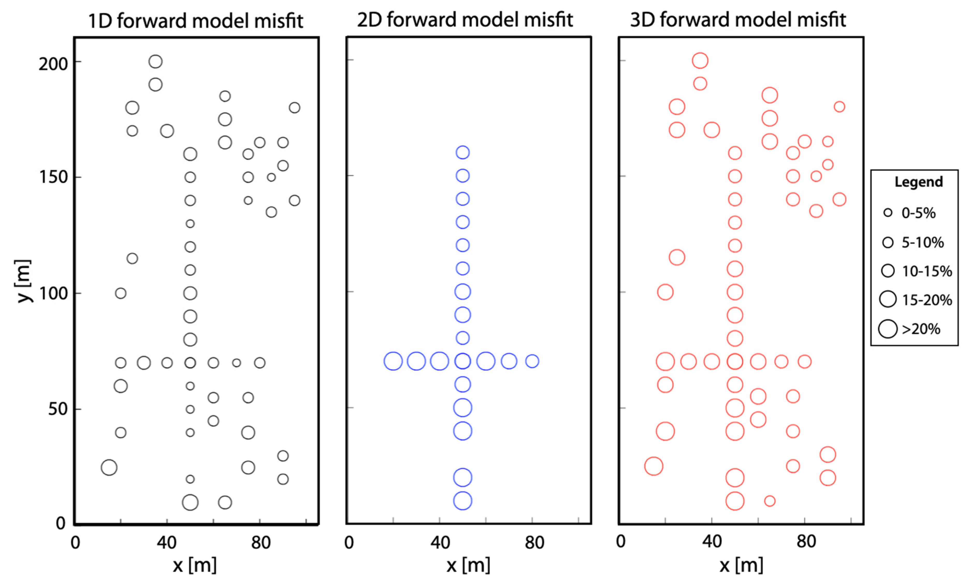
4.2. D and 3D Scenarios

In the previous section, we used the analytic solution of the TDEM forward problem to determine stitched 1D resistivity depth-profiles across the SE Malta study area. In this section, we use the FE analysis to compute frequency-domain responses of 2D and 3D models. The time-domain response is obtained by splining the frequency-domain response evaluated at each of the designated discrete frequencies. Subsequently, the set of time-domain responses are used as the input from which we develop a series of 2D and 3D forward model iterative adjustments. The best 2D and 3D models that result from this analysis are then further evaluated and interpreted. The adjustments are made by trial and error since insufficient computational resources are available to achieve an automated inversion process. Since a single forward run takes ~14 h of CPU time on our computational platform, and an automated inversion would require many thousands of forward runs, even with a highly efficient algorithm it is envisioned that both coarse-grained and fine-grained massive parallelization are a prerequisite for a fully 3D inversion. Such algorithmic development is beyond the scope of this study, but is definitely recommended for future work.
Figure 11 shows FE-calculated responses at two stations based on the fully 2-D model constructed from the stitched 1-D resistivity models shown in Figure 9. The calculated response at station A7 obtains from the alongshore 2D resistivity model in Figure 9a. This model allows spatial variations in resistivity only in the SE-NW direction. That criterion is kept for all soundings along Profile A. Similarly, the 2D lateral resistivity distribution used to compare with the observed soundings at each station along Profile B is based on the across-shore transect shown in Figure 9b. The yellow dots in Figure 11, left, represent the field response actually measured at station A7. The modeling result of the alongshore 2D structure, computed using the 3D FE code, is marked as the solid line. Another sounding at the intersection of the two transects, namely station B4, is displayed in green diamonds in Figure 11, right, with the corresponding across-shore 2-D model response shown by the solid line.
At the bottom of Figure 12, the step-off voltage response as a result of 3D forward modeling was computed at station locations A7 and B4. The 3D model shown at the top of Figure 12 is constructed by combining the 2D models from the three transects, namely Profiles A, B (in Figure 9) and C (Figure 10a). For the sake of better visualization, only a local portion of the complete 3D model that is indicative of the structure beneath station A7 is illustrated within the modeling-domain limits of {−40 m, 40 m}, {−40 m, 40 m} and {0 m, 60 m} in the x, y and z directions, respectively. Part of the model that is above ground surface up to 20 m high is also excluded for better visualization; the size of 10 × 10 m square TX loop is shown for scaling. The complete 3D model representing the subsurface structure beneath SE Malta, covering a surface area of 16,500 m2, is depicted in Figure 13. Some of the sounding points are included to better indicate the location and orientation of the 3D model with respect to the G-TEM survey layout. A brief sensitivity analysis is provided in Appendix B.
The computed misfit at each sounding location is plotted in terms of relative error, visualized using various circle sizes, for the 1D, 2D and 3D models. These misfit circles are shown in black, blue, and red, respectively (Figure 14). The misfits of the responses at gate 1 and 2 for all soundings are excluded from the display since the amplitude of the early-time responses is very large. The relative errors of the 2D model are shown only at the 21 stations of the reduced SE Malta 2018 dataset located along transects A and B. The reader should note that the misfit of the preferred 3D model at a given station may exceed the misfit of the 1D model at that station. The important point is that a single 3D model has been found that fits all the observations reasonably well, sometimes at the cost of locally increasing the misfit compared to a 1D model that strictly applies only to an individual station. The actual geoelectrical structure of the Earth is 3D rather than locally 1D beneath the G-TEM measurement stations.

5. Discussion

The results presented in this study suggest that the structure of the mean sea-level groundwater aquifer near the shore in SE Malta exhibits a lenticular shape, with decreasing thickness towards the coast. The combination of TDEM models derived from the summer 2018 and 2019 datasets shows distinct high-resistivity zones. These are interpreted as the signature of a brackish water-saturated geological medium, in this case corresponding to the LCL formation hosting the mean sea-level groundwater body.
Based on the preferred 3D TDEM model in Figure 13, the top layer up to 5 m deep is interpreted as the overlaying Globigerina Limestone and there is no geophysical indication of freshwater in this low-resistivity formation. We also find that the depth to the top of LCL and water table in the study area is 4–5 m. Our study is in good agreement with a regional groundwater modeling study (MARSOL, 2015) of the South Malta region which points out that the elevation of the top of the formation holding fresh groundwater is in the range +20 to −20 m with reference to mean sea level [37]. The zones of high resistivity below the depth of 4–5 m in the 2D and 3D models are indicative of a (moderately brackish) freshwater-bearing formation with resistivity in the range ρ ~10–100 Ω m (i.e., the purple-blue-cyan colors in Figure 13). The steeper base compared to the gentler top of the groundwater body is consistent with the geometry of a Ghyben-Herzberg-type lens. Below the freshwater region, from depths ~13–22 m down to the TDEM depth of investigation at 60 m, the underlying rocks situated beneath sea level are much less resistive, attaining values ρ ~1.25–2.5 Ω m (i.e., the green-yellowish green colors in Figure 13). These low resistivity (conductive) zones are indicative of a seawater-saturated formation. The shallow resistive freshwater lens sits on top of a more conductive formation, the latter being indicative of lateral landward movement of saltwater, i.e., intrusion. The boundary between the zones of high and low resistivity indicates the presence of the interface or transition zone along the two across-shore transects. Within the areas closest to the shoreline a mixing zone of freshwater and seawater appears to be present. Zones of moderate resistivity ρ ~5 Ω m are observed along the northeastern parts of the across-shore transects by the coast and this could be indicative of brackish groundwater.
In order to assess the groundwater quality implications of our model, we calculate the bulk resistivity of the fluid-saturated rock using Archie’s law [38] for various porosities of limestone assuming that all pore spaces are filled with freshwater with resistivity of 2 Ω m. This latter value is equal to the water resistivity found in a well located 2.5 km inland. For porosities of 10% and 15% we find 126.2 and 60.8 Ω m, respectively, as the formation bulk resistivity. These values of estimated resistivity are slightly higher than the range of those in the 3-D TDEM model ( ρ ~10–100 Ω m). In addition, we have estimated bulk resistivity for saturated limestone filled with seawater of 0.2 Ω m with 10%, and 15% porosities. These are 12.6 and 6.1 Ω m, respectively, which is also slightly higher than our model’s prediction of low resistivity seawater-saturated formations of 1.25–2.5 Ω m. As we move inland, our values are consistent with the borehole’s fluid resistivity saturating a formation of 10 to 15% porosity. Closer to the shoreline, the TDEM bulk resistivity is lower, reflecting more brackish water. Thus, the groundwater freshens as we move inland. Of course, Archie’s law is not a perfect petrophysical model for the fractured limestone lithology, since the law was founded on lab measurements made on clean sandstone cores, but an Archie-type calculation should be approximately correct.
To assess confidence in the spatial structure of our model, we also consider which of the model slabs indicative of the freshwater-bearing formation are best resolved based on the sensitivity analysis (see Appendix B for details). At the lower frequency of 100 Hz, the best-resolved slab is slab 3; whereas the responses from slabs 5, 6 and 7 are more sensitive to perturbations in their resistivity than the responses of slabs 1 and 2. At the high frequency 1 MHz, the misfit-change distribution indicates that changing a slab’s resistivity affects only the sounding that is situated directly over that slab. Slab 6 seems to be the most well-resolved slab at the intermediate frequency 31.6 kHz. Slabs located further inland appear to be not as well resolved as those closer to the sea. The latter are thin and more conductive relative to the thicker, more resistive inland slabs and it is well known that terrestrial TDEM better resolves thin conductive layers.
We do not have sufficient data coverage to infer a possible offshore extension of the freshwater aquifer at the SE Malta study site. The landward encroachment of seawater decreases the resistivities of the near-coastline region and possibly interacts with the fresh groundwater of the MSLA. There are unpublished ground-penetrating radar (GPR) data that appear to show infiltrated meteoric water trapped in fractures above water table in some areas of the study site [39]. More across-shore measurements throughout Malta are recommended in order to investigate the lateral subsurface geoelectrical variation in the direction perpendicular to the coast.

6. Conclusions

This study demonstrates the utility of the TDEM geophysical method along with 1D, 2D and 3D forward modeling as a means to study coastal freshwater aquifers in water-scarce regions. Here we image the geometry of the onshore aquifer within the permeable Lower Coralline Limestone formation along the SE Malta coast. Our results show 2D and 3D resistivity models found by iterative adjustments of FE forward modeling. The final preferred 3D model provides information to depth of 60 m, covering an area of ~16,500 m2 and shows diagnostic spatial variations in subsurface electrical resistivity. The geophysical modeling provides a basis for determining important characteristics of the MSLA that fit our observations, namely the decreasing thickness of fresh groundwater bodies towards the coastline. Zones of fresh groundwater have been identified, but these are located preferentially inland from the coast. Thus, there is no indication from the electromagnetic data of a robust offshore extension of the MSLA at this location. However, it is argued that method that we used can be applied across the entire Maltese archipelago to better constrain the geometry, dimensions and distribution of terrestrial and coastal aquifers providing valuable information for future water management of the stressed groundwater reserves of Malta.

Author Contributions

Conceptualization, A.M., B.A.W., P.P. and M.E.E.; P.P. prepared the manuscript with contributions from all co-authors; M.E.E., A.M., Z.F. and B.A.W. collected the G-TEM data during summer 2018 fieldwork; P.P., M.E.E., A.M. and B.A.W. collected the 2019 dataset; P.P. analyzed the data with supervision from M.E.E.; M.E.E., A.M., A.H. and M.J. contributed to the discussion on the modeling results. All authors have read and agree to the published version of the manuscript.

Funding

This project has received funding from the European Research Council (ERC) under the European Union’s Horizon 2020 research and innovation programme (grant agreement No 677898 MARCAN).

Acknowledgments

The authors are grateful to Rob Evans for helping out in the field work in June, 2019. We would like to thank the two anonymous reviewers for valuable comments that have greatly improved the paper. We also thank GEOMAR for travel and equipment transportation support during the SMART summer school 2019 at the University of Malta. SMART is funded by GEOMAR and the Helmholtz Association of German Research Centres – European Partnering Initiative.

Conflicts of Interest

The authors declare no conflict of interest.

Appendix A. Receiver Gates and Time

The G-TEM receiver records the characteristics of transient response by sampling it at 20 or 30 sequential time intervals or gates. The gates are logarithmically-spaced times that fill the measurement period and their widths (separation) exponentially increase with time [40]. Table A1 lists the center time of each gate that occurs after TX shut-off for repetition rate of 237.5 Hz at 20-gates acquisition mode.
Table A1. Gate center times.
GateTimeGateTime
(μs)(μs)
16.8131177.94
28.6881299.38
311.1313126.7
414.1914166.4
518.0715206
623.0616262.8
729.4417355.2
837.5618427.7
947.9419545.6
1061.1320695.9

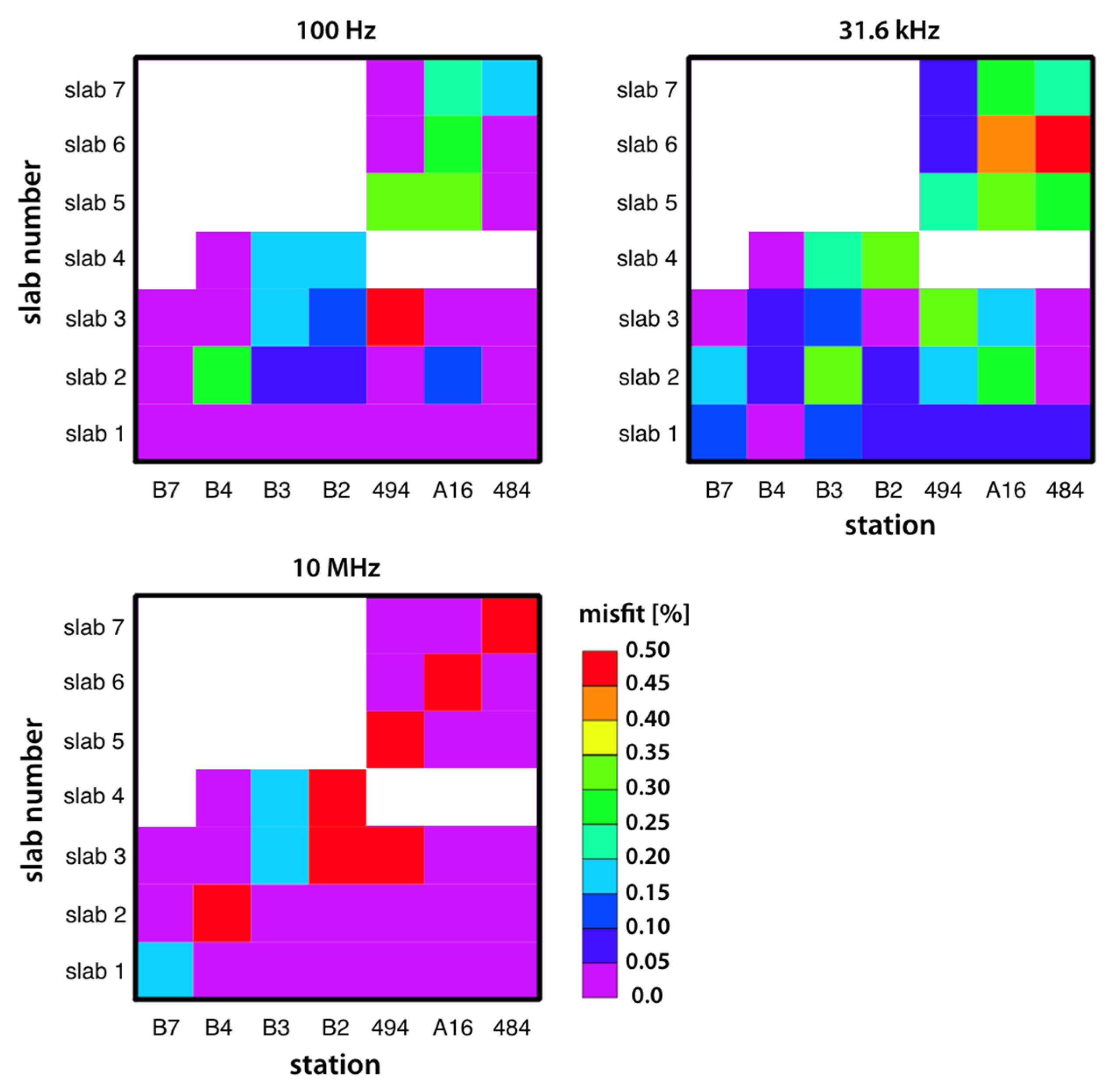
Appendix B. Sensitivity Analysis

It is of interest to examine which of the slabs indicative of the freshwater-bearing formation responds most sensitively to the time-domain electromagnetic excitation. Conducting a sensitivity analysis provides information about how small perturbations to an independent variable, in this case a slab resistivity, affect the 3D model’s overall misfit. Herein, the resistivity of each slab is subjected to a 5% decrease and the 3D response re-computed, with only one slab changed at a time. We compute the vertical magnetic fields at three different frequencies to determine the changes in subsequent responses after each slab’s resistivity is changed compared with the responses of the unperturbed preferred model shown in Figure 13. The choices of 100 Hz, 31.6 kHz, and 10 MHz generate low, medium, and high frequency responses, respectively. Seven slabs with various resistivities ranging from 8.3 to 100 Ω m are chosen and the corresponding seven sounding locations on the surface nearest the center of each slab are selected for monitoring the change of computed responses (see Figure A1). For example, station B7 is underlain by slab 1, station B4 overlies slab 2, station B3 is above slab 3, and so on. The computed misfit resulting from a model that includes a perturbation in a slab’s resistivity is displayed in terms of relative change, illustrating using a color plot for the three different frequencies in Figure A2.
Figure A1. Illustration of the location of selected slabs (numbered 1–7) that are suggestive of a water-bearing formation, and the TDEM sounding locations where the sensitivity analysis is performed. Value of unperturbed resistivity is shown for each slab.
Water 12 01566 g0a1
At low frequency (100 Hz), Figure A2 top left, the changes in frequency-domain responses at each station are mainly due to the directly underneath slab and to the neighboring slabs. This is indicated by the larger values of percentage misfit mainly along the diagonal of the plot. An exception is the change caused by decreasing in resistivity of slab 1 that did not appreciably affect the misfit at any of the 7 stations. Surprisingly, the sounding 494, beneath slab 5, is most sensitive to the decrease of resistivity of slab 3 at frequency of 100 Hz. At moderate frequency (31.6 kHz), Figure A2 top right, slab 1 has a minor impact on the data if its resistivity decreases. The misfit plot shows how the change in one slab’s resistivity affects almost all the surrounding stations by different amounts. Moreover, the change in resistivity of slab 6 has a large effect on observed responses at the soundings A16 and 484, located above slabs 6 and 7, respectively. At high frequency 10 MHz, bottom left of Figure A2, the misfit-change distribution indicates that decreasing a slab’s resistivity is likely to affect only the sounding that situated over that slab. This result is not surprising since the footprint of a TDEM sounding is smallest at high frequencies.
Figure A2. Response misfits for 100 Hz, 31.6 kHz and 10 MHz. Color plot denotes a relative change in percentage misfit for examples of seven soundings after each slab’s resistivity decreases by 5%. The white region in each plot signifies that there is no effect from perturbation to a particular slab detected by that sounding location. The misfits over 0.25% at each frequency are considered significant by rough estimation, and this will affect the 1D, 2D and 3D modelling misfits of transient EM responses in Figure 14.
Water 12 01566 g0a2

References

  1. Post, V.E.; Groen, J.; Kooi, H.; Person, M.; Ge, S.; Edmunds, W.M. Offshore fresh groundwater reserves as a global phenomenon. Nature 2013, 504, 71–78. [Google Scholar] [CrossRef] [PubMed]
  2. Jones, E.; Qadir, M.; van Vliet, M.T.H.; Smakhtin, V.; Kang, S.M. The state of desalination and brine production: A global outlook. Sci. Total Environ. 2019, 657, 1343–1356. [Google Scholar] [CrossRef] [PubMed]
  3. Archie, G.E. Electrical Resistivity Log as an Aid in Determining Some Reservoir Characteristics. Trans. AIME 1942, 146, 54–67. [Google Scholar] [CrossRef]
  4. Nabighian, M.N.; Macnae, J.C. Time Domain Electromagnetic Prospecting Methods. In Investigations in Geophysics No 3. Electromagnetic Methods in Applied Geophysics; Nabighian, M.N., Ed.; Society of Exploration Geophysicists: Tulsa, OK, USA, 1991; pp. 427–514. [Google Scholar]
  5. Everett, M.E.; Chave, A.D. On the physical principles underlying electromagnetic induction. Geophysics 2019, 84, w21–w32. [Google Scholar] [CrossRef]
  6. Everett, M.E. Theoretical Developments in Electromagnetic Induction Geophysics with Selected Applications in the Near Surface. Surv. Geophys. 2012, 33, 29–63. [Google Scholar] [CrossRef]
  7. Fitterman, D.V. Tools and techniques: Active-source electromagnetic methods. In Resources in the Near-Surface Earth, Treatise on Geophysics; Slater, L., Ed.; Elsevier B. V.: Amsterdam, The Netherlands, 2015; Volume 11, pp. 295–333. [Google Scholar]
  8. Yogeshwar, P.; Tezkan, B. Two-dimensional basement modeling of central loop transient electromagnetic data from the central Azraq basin area, Jordan. J. Appl. Geophys. 2017, 136, 198–210. [Google Scholar] [CrossRef]
  9. Fitterman, D.V.; Stewart, M.T. Transient electromagnetic sounding for groundwater. Geophysics 1986, 51, 995–1005. [Google Scholar] [CrossRef]
  10. Kafri, U.; Goldman, M.; Lang, B. Detection of subsurface brines, freshwater bodies and the interface configuration in-between by the time domain electromagnetic method in the Dead sea rift, Israel. Environ. Geol. 1997, 31, 42–49. [Google Scholar] [CrossRef]
  11. Danielsen, J.E.; Auken, E.; Jørgensen, F.; Søndergaard, V.; Sørensen, K.I. The application of the transient electromagnetic method in hydrogeophysical surveys. J. Appl. Geophys. 2003, 53, 181–198. [Google Scholar] [CrossRef]
  12. Siemon, B.; Christiansen, A.V.; Auken, E. A review of heliopter-borne electromagnetic methods for groundwater exploration. Near Surf. Geophys. 2009, 7, 629–646. [Google Scholar] [CrossRef] [Green Version]
  13. Costabel, S.; Siemon, B.; Houben, G.; Günther, T. Geophysical investigation of a freshwater lens on the island of Langeoog, Germany—Insights from combined HEM, TEM and MRS data. J. Appl. Geophys. 2017, 136, 231–245. [Google Scholar] [CrossRef] [Green Version]
  14. Kalisperi, D.; Kouli, M.; Vallianatos, F.; Soupios, P.; Kershaw, S.; Lydakis-Simantiris, N. A Transient ElectroMagnetic (TEM) Method Survey in North-Central Coast of Crete, Greece: Evidence of Seawater Intrusion. Geosciences 2018, 8, 107. [Google Scholar] [CrossRef] [Green Version]
  15. Morgan, L.K.; Werner, A.D.; Patterson, A.E. A conceptual study of offshore fresh groundwater behaviour in the Perth Basin (Australia): Modern salinity trends in a prehistoric context. J. Hydrol. Reg. Stud. 2018, 19, 318–334. [Google Scholar] [CrossRef]
  16. Yu, X.; Michael, H.A. Offshore Pumping Impacts Onshore Groundwater Resources and Land Subsidence. Geophys. Res. Lett. 2019, 46, 2553–2562. [Google Scholar] [CrossRef]
  17. Pedley, H.M.; House, M.R.; Waugh, B. The geology of Malta and Gozo. Proc. Geol. Ass. 1976, 87, 325–341. [Google Scholar] [CrossRef]
  18. Micallef, A.; Foglini, F.; Le Bas, T.; Angeletti, L.; Maselli, V.; Pasuto, A.; Taviani, M. The submerged paleolandscape of the Maltese Islands: Morphology, evolution and relation to Quaternary environmental change. Mar. Geol. 2013, 335, 129–147. [Google Scholar] [CrossRef]
  19. Directorate, O.E. Geological Map of the Maltese Islands; Office of the Prime Minister: Valletta, Malta, 1993.
  20. Illies, J.H. Graben formation—The Maltese Islands, a case study. Tectonophysics 1981, 73, 151–168. [Google Scholar] [CrossRef]
  21. Galdies, C. The Climate of Malta: Statistics, Trends and Analyses 1951–2010; National Statistics Office: Valletta, Malta, 2013.
  22. FAO. Malta Water Resources Review; FAO: Rome, Italy, 2006; Available online: http://www.fao.org/3/a-a0994e.pdf (accessed on 18 February 2020).
  23. Stuart, M.E.; Maurice, L.; Heaton, T.H.E.; Sapiano, M.; Micallef Sultana, M.; Gooddy, D.C.; Chilton, P.J. Groundwater residence time and movement in the Maltese islands—A geochemical approach. Appl. Geochem. 2010, 25, 609–620. [Google Scholar] [CrossRef] [Green Version]
  24. MARSOL. Demonstrating Managed Aquifer Recharge as a Solution to Water Scarcity and Drought Characterisation of the Sea-Level Aquifer System in the Malta South Region; Institution of Applied Geosciences: Darmstadt, Germany, 2016; Available online: http://www.marsol.eu/files/marsol_d10-4_malta-groundwater-model.pdf (accessed on 14 January 2020).
  25. Bakalowicz, M.; Mangion, J. The limestone aquifers of Malta: Their recharge conditions from isotope and chemical surveys. Hydrology of the Mediterranean and Semiarid Regions (Proceedings of an international symposium held at Montpellier. Int. Assoc. Hydrol. Sci. Publ. 2003, 278, 49–54. [Google Scholar]
  26. Malta Environment and Planning Authority and the Malta Resources Authority. The Water Catchment Management Plan for the Maltese Islands; Malta Environment and Planning Authority and the Malta Resources Authority: Marsa, Malta, 2011; Available online: https://era.org.mt/en/Documents/1st%20WCMP_final.pdf (accessed on 16 January 2020).
  27. Mangion, J.; Sapiano, M. The Mean Sea Level Aquifer, Malta and Gozo. In Natural Groundwater Quality; Blackwell Publishing: Ames, IA, USA, 2008; pp. 404–420. [Google Scholar]
  28. BRGM. Study of the Fresh Water Resources of Malta; Appendix 7: Water Quality and Environmental Aspects, R 33691 EAU 4S 91; BRGM: Orleans, France, 1991. [Google Scholar]
  29. Malta Environment and Planning Authority. Minerals Subject Plan for the Maltese Islands 2002; Entec UK Ltd.: London, UK, 2003. [Google Scholar]
  30. Spies, B.R. Depth of investigation in electromagnetic sounding methods. Geophysics 1989, 54, 872–888. [Google Scholar] [CrossRef]
  31. Constable, S.C.; Parker, R.L.; Constable, C.G. Occam’s inversion: A practical algorithm for generating smooth models from electromagnetic sounding data. Geophysics 1987, 52, 289–300. [Google Scholar] [CrossRef]
  32. Ward, S.H.; Hohmann, G.W. Electromagnetic Theory for Geophysical Applications, in Electromagnetic Methods in Applied Geophysics Theory. Soc. Explor. Geophys. 1988, 1, 131–311. [Google Scholar]
  33. Everett, M.E. Near-Surface Applied Geophysics; Cambridge University Press: Cambridge, UK, 2013. [Google Scholar]
  34. Chave, A.D. Numerical integration of related Hankel transforms by quadrature and continued fraction expansion. Geophysics 1983, 48, 1671–1686. [Google Scholar] [CrossRef] [Green Version]
  35. Badea, E.A.; Everett, M.E.; Newman, G.A.; Biro, O. Finite-element analysis of controlled-source electromagnetic induction using Coulomb-gauged potentials. Geophysics 2001, 66, 786–799. [Google Scholar] [CrossRef]
  36. Stalnaker, J.L.; Everett, M.E.; Benavides, A.; Pierce, C.J. Mutual induction and the effect of host conductivity on the EM induction response of buried plate targets using 3-D finite-element analysis. IEEE Trans. Geosci. Remote Sens. 2006, 44, 251–259. [Google Scholar] [CrossRef]
  37. MARSOL. Demonstrating Managed Aquifer Recharge as a Solution to Water Scarcity and Drought Characterisation of the Sea-Level Aquifer System in the Malta South Region; Institution of Applied Geosciences: Darmstadt, Germany, 2015; Available online: http://www.marsol.eu/files/marsol_d10-1_msla-characterisation.pdf (accessed on 11 January 2020).
  38. Fofonoff, N.P.; Millard, J.R.C. Algorithms for the computation of fundamental properties of seawater. In UNESCO Technical Papers in Marine Sciences; UNESCO: Paris, France, 1983; Volume 44. [Google Scholar]
  39. Enzo Rizzo. Personal communication. Available online: https://hyfrew.wordpress.com/ (accessed on 1 May 2020).
  40. Geonics. G-TEM Operating Manual; Geonics Limited: Mississauga, ON, Canada, 2016. [Google Scholar]
Figure 1. (a) Geological map of the island of Malta and an inset map showing location of Malta in the Mediterranean Sea as a red square. Modified from Geological Map of Maltese Islands, 1993 [19]. Black lines denote faults. The lithological profile is provided in the right panel. Study site is shown as blue square. (b) Detail of the study site in SE Malta; transect A is aligned NW–SE and B is aligned NE–SW. Time-domain electromagnetic (TDEM) soundings are marked as squares with black squares inside; the difference in colors denotes different acquisition dates. White symbols show TDEM sounding locations from July 2018. Additional soundings investigated during June and July 2019 are indicated by cyan and purple symbols, respectively.
Water 12 01566 g001
Figure 2. Field deployment of Geonics G-TEM geophysical equipment in SE Malta.
Water 12 01566 g002
Figure 3. Location of TDEM soundings and four 2D transects are shown. A symbol denotes position of each sounding and differences in colors refer to different measurement dates. TDEM soundings deployed during July 2018, June 2019, and July 2019 are indicated by black-and-white, black-and-cyan and black-and-purple symbols, respectively.
Water 12 01566 g003
Figure 4. Example of G-TEM data shown as square symbols and the computed resistivity depth profile displayed as a curve passing through all data points with root mean square (RMS) misfit 6.8% (left); the fitted model is marked as the dark green line while the red line is the starting model (right).
Water 12 01566 g004
Figure 5. G-TEM data from 23 soundings in SE Malta. (a) All 16 soundings in profile A; (b) soundings from the 7 stations belonging to Profile B.
Water 12 01566 g005
Figure 6. (left) 1D analytic forward result for station A2, A4 to A9 shown as the black solid line; (right) The resistivity model corresponds to the response (sold line) displayed in the left panel.
Water 12 01566 g006
Figure 7. Decay curves of some measured G-TEM soundings at the western section of study area. An unusual decay at station 432 denoted as black squares may be due to a localized highly-conductive body.
Water 12 01566 g007
Figure 8. 1D forward modeling result for station 428, 429, 430 and B3 shown as a black line (see column beneath B3 in Figure 9b for the model.).
Water 12 01566 g008
Figure 9. Stitched version of resistivity profiles obtained from 1D forward modeling results of the 2018 (a) alongshore Profile A and (b) across-shore Profile B surveys. The white line provides a rough guide to the geometry of the thinning of the freshwater lens towards the coast, where it becomes brackish to mildly saltwater.
Water 12 01566 g009
Figure 10. Stitched version of resistivity models from (a) Profile C along the western boundary and (b) Profile D in the northern part of the study site. The white line provides a rough guide to the geometry of the thinning of the freshwater lens towards the coast, where it becomes brackish to mildly saltwater.
Water 12 01566 g010
Figure 11. 2D modeling results of station A7 and B4 from left to right. A computed step-off voltage from 3D forward modeling code at cross-section point of two transects is shown as a black line.
Water 12 01566 g011
Figure 12. (a) 3D resistivity model showing the subsurface geoelectrical distribution beneath A7 and B4; (b) The computed step-off voltage according to the resistivity model in (a) is displayed as a black line.
Water 12 01566 g012
Figure 13. The preferred 3D model representing the subsurface geoelectrical structure beneath study site in SE Malta.
Water 12 01566 g013
Figure 14. Misfit of 1D, 2D and 3D models, from left to right. Size of circle represents a relative error for each sounding. Only 21 points of misfits are shown for 2D model along 2018 dataset.
Water 12 01566 g014

