Experimental Study and Numerical Simulation of Gas–Liquid Two-Phase Flow in Aeration Tank Based on CFD-PBM Coupled Model

Abstract

Gas–liquid two-phase flow directly determines the efficiency and stability of the aeration tank. In this paper, a gas–liquid two-phase testbed is built to explore the aeration performance and internal flow in an aeration tank, including an inverted-umbrella impeller (immersion depth of 0 mm, rotational speed of 250 r/min). Also, the running process is simulated by computational fluid dynamics (CFD) with a population balance model (PBM), and mass transfer coefficient is compared to the experiment. The experimental results show that there is a big difference in bubble diameter, ranging from 0.4 to 1.6 mm. The simulation shows that the impeller intensely draws air above the free surface into the shallow liquid, and the circulation vortex entrains it to the bottom areas faster. Compared with the experiment, the simulated interfacial area and standard oxygen mass transfer coefficient is 12% more and 3% less, respectively. The results reveal that CFD-PBM coupled model can improve the accuracy of calculation, resulting in the simulation of gas–liquid two-phase flow.

1. Introduction

In urban wastewater treatment, the primary process for the treatment of nitrogen and organic compounds in wastewater is activated sludge. In the process, aeration consumes up to 70% of the total energy expenditure of the plant. There are different kinds of aeration equipment, such as the rotating brush, rotating disk, inverted-umbrella aerator, and so on. The inverted-umbrella aerator has various advantages which include a simple structure, strong oxygenation capacity and high-power efficiency. Moreover, it combines the use of oxygenation and stirring functions [1]. Thus, it has become one of the most widely used aeration equipment in oxidation ditch. The inverted-umbrella aerator throws the sewage into the air and is involved in air. The bottom of the impeller and suction side of blades generate negative pressure and suck air, which makes the bubble size in the aeration tank vary widely. Therefore, some complex gas–liquid two-phase flow characteristics are involved in the aeration tank, such as self-aeration. It is necessary to conduct two-phase flow analysis more accurately on the local hydrodynamics of the aeration tank to ensure a reliable and effective treatment in such facilities [2].

Experimentation is always an important method to study two-phase flow in the aeration tank. Burges [3,4] measured the bubble size, liquid velocity and turbulence in the tube through a conductance probe and optical fiber probe. Liu [5] established the bubble feature extraction method through high-speed photography and MATLAB image processing technology. The bubble characteristics (bubble size and distribution, etc.) were extracted precisely. Lee [6] photographed the movement of bubbles in an oxidation ditch using high-speed photography and obtained the speed of bubbles under different aspect ratios. Xing [7] measured the total gas content and volume fraction of small and large bubbles in the bubble column through dynamic gas separation.

In recent years, with the development of computer technology, great progress has been made in the study of computational fluid dynamics (CFD) in the aeration tank (bubble size, gas holdup, mass transfer coefficient). Various approaches have been suggested for solving the two-phase flow problem, and modeling may be attempted at various levels of sophistication [8]. Milelli [9] and Deen [10] simulated the turbulence of the liquid phase combining the Euler-Euler model, Large Eddy Simulation (LES) model and the k-epsilon (k–ε) model. The results revealed that LES compares better with the experimental data. Liu [11] simulated gas–liquid two-phase flow in the aeration tank through the volume of fluid (VOF) model. The flow field, streamline distribution, velocity distribution, free-surface deformation and turbulence kinetic energy were analyzed at several vertical positions. Karpinska et al. [12] built a gas–liquid two-phase flow model in an oxidation ditch and studied the volume distribution of the gas phase. However, the VOF model takes the free surface as the cylinder head interface, which ignores the vertical movement of the surface. Zhang [13] simulated the flow field in the seawater desulfurization aeration tank through the two-fluid model and studied the influence of different air velocity on the mixture of gas–liquid.

In the aeration tank, bubbles are coalesced by turbulence and trailing vortex due to the influence of surface tension, lift and drag force. When the inertia force of turbulent vortices is greater than the force caused by the surface tension of bubbles, bubbles continue to deform until they break into smaller sized bubbles [14]. In the traditional CFD method, the size of bubbles is considered to be constant, and the bubble coalescence and bubble breakup are not considered. It is impossible to simulate the inter-phase area of gas–liquid two-phase flow and accurately predict the mass transfer behavior.

Many scholars have considered the coalescence and breakup effects of bubbles through the population balance model (PBM) and studied gas–liquid two-phase flow coupling with the Euler-Euler two-fluid model [15]. Gupta [16] carried out a numerical simulation of a rectangular bubble column though CFD-PBM. The effects of different coalescence, fragmentation, lift and virtual mass force on the flow and gas holdup in an aeration tank were analyzed. Xu [17] studied hydrodynamic properties of the gas–liquid two-phase velocity field distribution, gas holdup and bubble size in the bubble column at different superficial gas velocity through CFD-PBM. Wang [18] presented a Euler-Euler two-fluid model coupled with the population balance model and simulated the gas–liquid two-phase flow field of four different inlets at the bottom of the bubble column. The simulated results show that the Euler-Euler model with PBM is consistent with the experimental results and better than those models with a single bubble diameter. Wang L. [19] simulated the gas–liquid mass transfer in a bubble column under homogeneous and heterogeneous flow regime with a CFD-PBM coupled model and gas–liquid mass transfer model. The simulation results show that the CFD-PBM coupled model is an effective method to predict the hydrodynamics, bubble size distribution, interfacial area and gas–liquid mass transfer rate of the bubble column. Wang [20] reviewed the modelling and simulation of bubble column reactors using CFD coupled with PBM. The models of bubble breakup and coalescence caused by different mechanisms were discussed.

In summary, the previous research on the characteristics of gas–liquid two-phase flow mainly focused on the external ventilation (such as bubble columns, etc.), and there were few researchers who studied gas–liquid two-phase flow of the self-aeration model, such as the inverted-umbrella aerator. In addition, the coalescence and overlapping of bubbles will lead to bubble adhesion, which makes it more difficult to accurately simulate the gas–liquid two-phase in the aeration tank with PBM. To solve this problem, the distribution of bubbles in the tank is obtained by combining high-speed photography and image processing methods, and the gas–liquid two-phase and mass transfer coefficients are calculated based on the CFD-PBM coupled model.

2. Materials and Methods

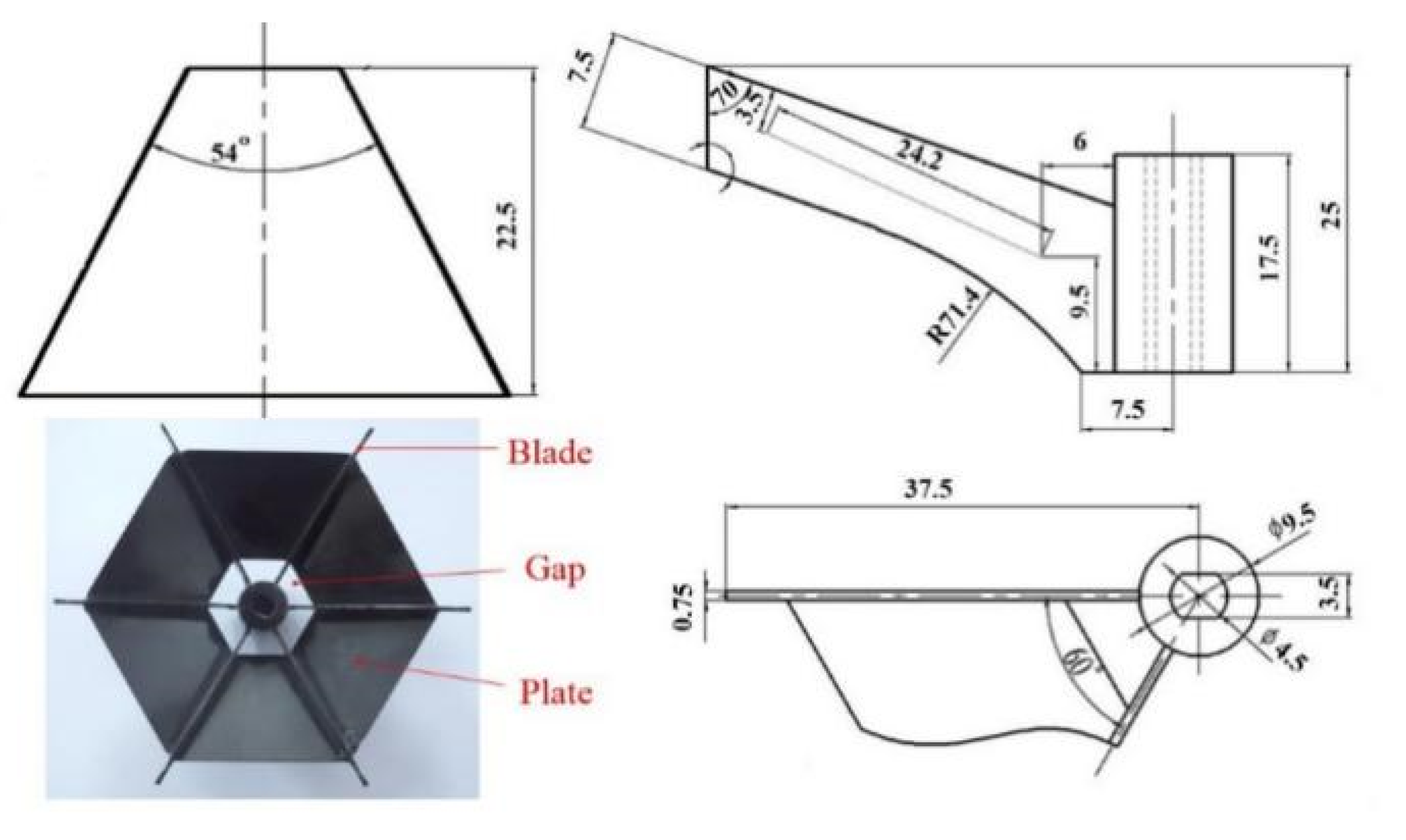
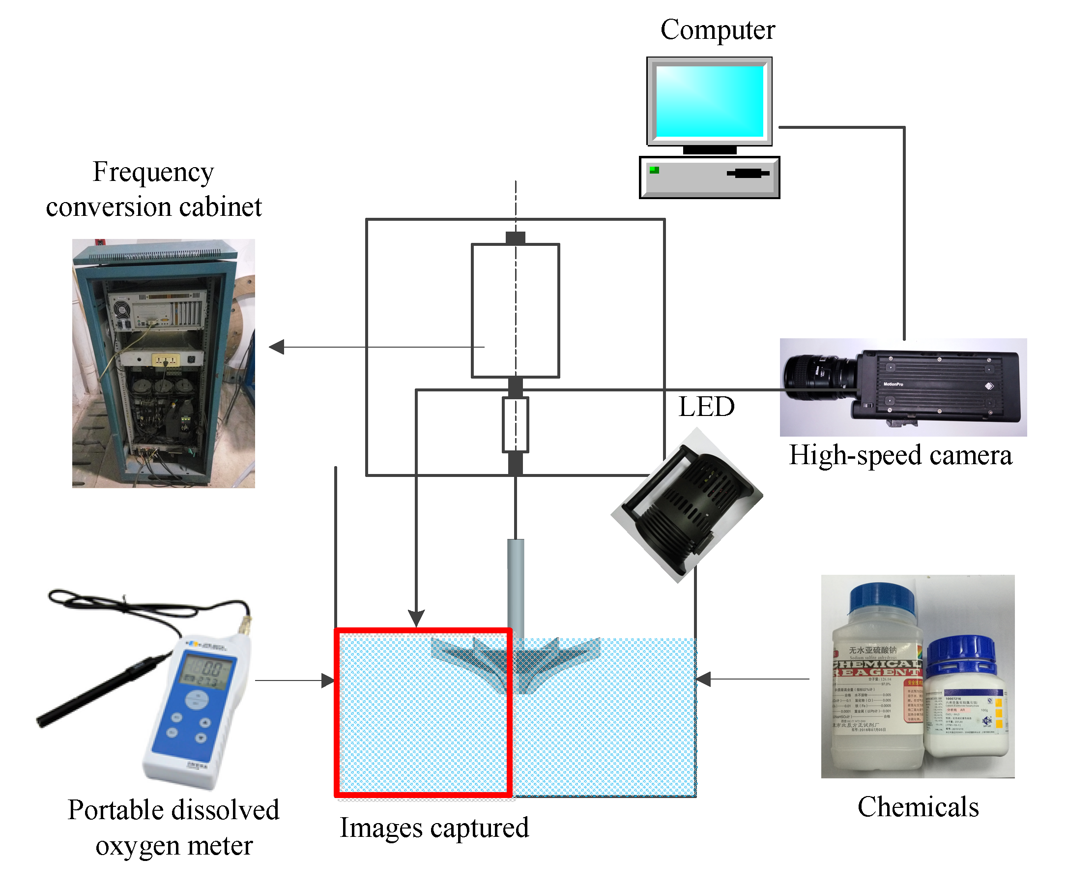
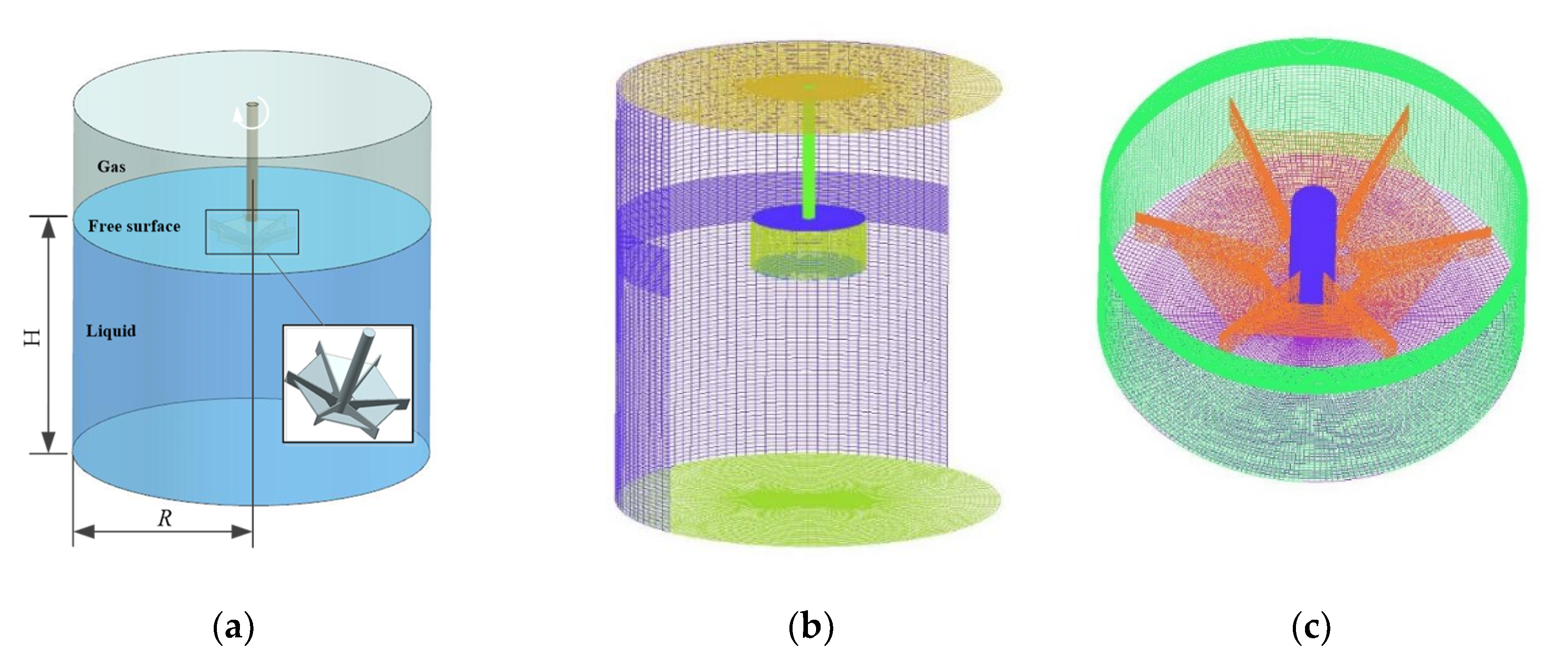
The test system consists of a circular aeration tank, inverted-umbrella aerator, frequency controller, motor, portable dissolved oxygen meter, Light Emitting Diode (LED), high-speed camera, computer, and so on. The diameters of the impeller and the tank are 75 and 300 mm, respectively. In the test, the immersion depth is 0 mm; that is, the highest point of the blade is equal to the free surface. The liquid depth in the aeration tank is 200 mm, and the rotational speed of the inverted-umbrella aerator is 250 rpm. The geometric parameters of the impeller are shown in Figure 1.

The schematic diagram of the test system is shown in Figure 2. The dissolved oxygen concentration is collected by a portable dissolved oxygen meter, the detailed description of which is shown in

Table 1. Detailed description of the portable dissolved oxygen meter.

Name	Type	Range	Precision	Manufacturer
Portable dissolved oxygen meter	JPB-607A	0~20 mg/L	±0.3 mg/L	Lei Ci in Shanghai

. The chemicals are Na₂SO₃ (deoxidizer) and CoCl₂·6(H₂O) (catalyst). The high-speed camera is used to capture the characteristic distribution of bubbles in the aeration tank, and the specific parameters of the camera are shown in

Table 2. Specific parameters of the camera.

Projects	Technical Index
Maximum resolution	1024 × 1024
Pixel size/μm	14 × 14
Memory/G	16
Continuous shooting time/s	45
Whole resolution shooting speed/Frames Per Second (fps)	4000
Reduced resolution shooting speed/fps	256,000

. The flow on both sides of the aerator has the same law and shows approximately symmetrical distribution. Therefore, the left area is selected to study gas–liquid two-phase flow distribution in the tank.

3. Test Results and Discussion

3.1. Results and Discussion of Dissolved Oxygen Concentration Test

The experimental result of dissolved oxygen concentration is shown in

Table 3. Dissolved oxygen concentration.

Time (s)	Concentration (mg/L)	Time (s)	Concentration (mg/L)	Time (s)	Concentration (mg/L)	Time (s)	Concentration (mg/L)
0.5	0.1	5	3.3	9.5	5.4	14	6.8
1	0.4	5.5	3.5	10	5.6	14.5	7.0
1.5	0.8	6	3.8	10.5	5.7	15	7.1
2	1.2	6.5	4.0	11	5.9	15.5	7.2
2.5	1.6	7	4.3	11.5	6.1	16	7.3
3	1.9	7.5	4.5	12	6.2	16.5	7.4
3.5	2.3	8	4.7	12.5	6.4	17	7.5
4	2.6	8.5	5.0	13	6.5	17.5	7.6
4.5	3.0	9	5.2	13.5	6.7	18	7.6

.

The oxygen mass transfer coefficient, k_La, of the inverted-umbrella aerator is calculated through dissolved oxygen concentration. The oxygen mass transfer coefficient, k_La, is the mass of oxygen transferred from gas phase to liquid phase in unit volume in unit time. The mass transfer of oxygen plays a decisive role in the biochemical reaction in the aeration tank. Therefore, the oxygen mass transfer coefficient, k_La, is often used to indicate the aeration performance of the aerator.

The variation of dissolved oxygen concentration is as follows:

$$\frac{\mathrm{dC}}{\mathrm{dt}}={\mathrm{k}}_{\mathrm{L}}\mathrm{a}\left({\mathrm{C}}_{\mathrm{s}}-\mathrm{C}\right)$$

(1)

where, dC/dt is the oxygen transfer rate, mg/(L min). k_La is the oxygen mass transfer coefficient, min⁻¹. Cs is the oxygen saturation concentration under the experimental conditions, mg/L. C is the dissolved oxygen concentration at time T, mg/L.

Equation (1) is integrated:

$${\mathrm{k}}_{\mathrm{L}}\mathrm{a}=\frac{\ln \left({\mathrm{C}}_{\mathrm{s}}-{\mathrm{C}}_{\mathrm{t}1}\right)-\ln \left({\mathrm{C}}_{\mathrm{s}}-{\mathrm{C}}_{\mathrm{t}2}\right)}{{\mathrm{t}}_2-{\mathrm{t}}_1}$$

(2)

where, C_t1 is the dissolved oxygen concentration at time T₁, mg/L. C_t2 is the dissolved oxygen concentration at time T₂, mg/L.

The dissolved oxygen concentration in the aeration tank is measured at the immersion depth of 0 mm and rotational speed of 250 r/min when the liquid level H is 200 mm. The time history plot of the dissolved oxygen concentration is obtained.

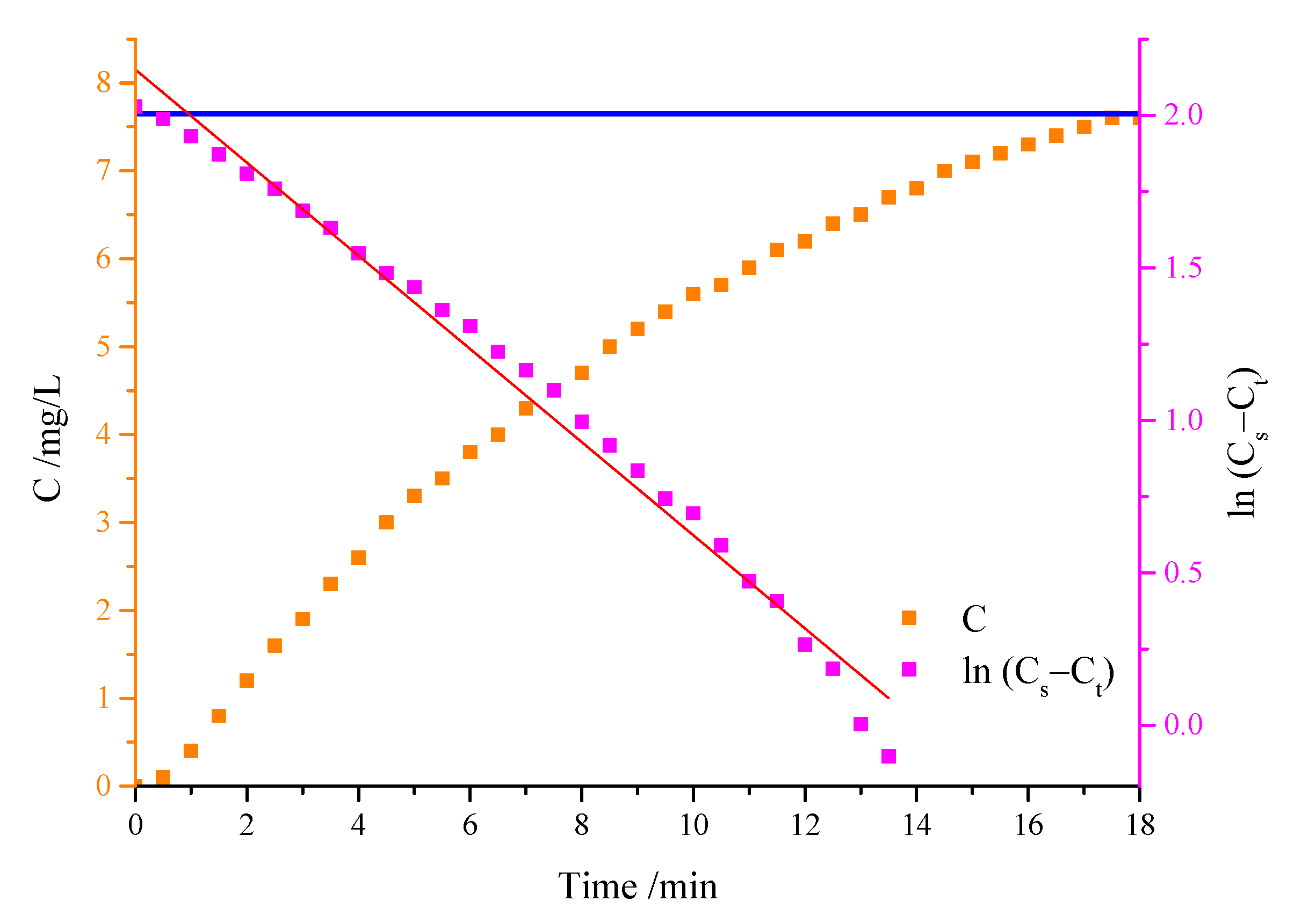
According to Equation (2), the oxygen mass transfer coefficient, k_La, is linearly related to the logarithmic concentration ln (C_s − C_t), k_La is the opposite of the slope of the time history plot of logarithmic concentration ln (C_s − C_t). The dissolved oxygen concentration is converted into logarithmic concentration, and the scatter plot is made. Scattered points are fitted linearly. The curve fitting has high accuracy, and the coefficient of determination R² reaches more than 0.98. The curve of dissolved oxygen concentration and the fitting results are shown in Figure 3 (the blue line in the figure is the saturated dissolved oxygen concentration, and the magenta line is the slope of ln (C_s − C_t)).

The liquid is tested at different temperatures. In order to eliminate the effect of temperature on the accuracy of the experiment, temperature correction is carried out. The correction formula is as follows [21]:

$${\mathrm{k}}_{\mathrm{L}}{\mathrm{a}}_{\left(20\right)}={\mathrm{k}}_{\mathrm{L}}{\mathrm{a}}_{\left(\mathrm{T}\right)}\times {1.024}^{20-\mathrm{T}}$$

(3)

where, T is the liquid temperature, °C. k_La _(T) is oxygen mass transfer coefficient at test liquid temperature T, min⁻¹. 1.024 is the correction coefficient.

Test temperature T is 28.9 °C at an immersion depth of 0 mm, and the standard oxygen mass transfer coefficient k_La₍₂₀₎ is 0.1237 min⁻¹ when the rotational speed of the impeller is 250 r/min.

3.2. Results and Discussion of High-Speed Photography

3.2.1. Image Processing

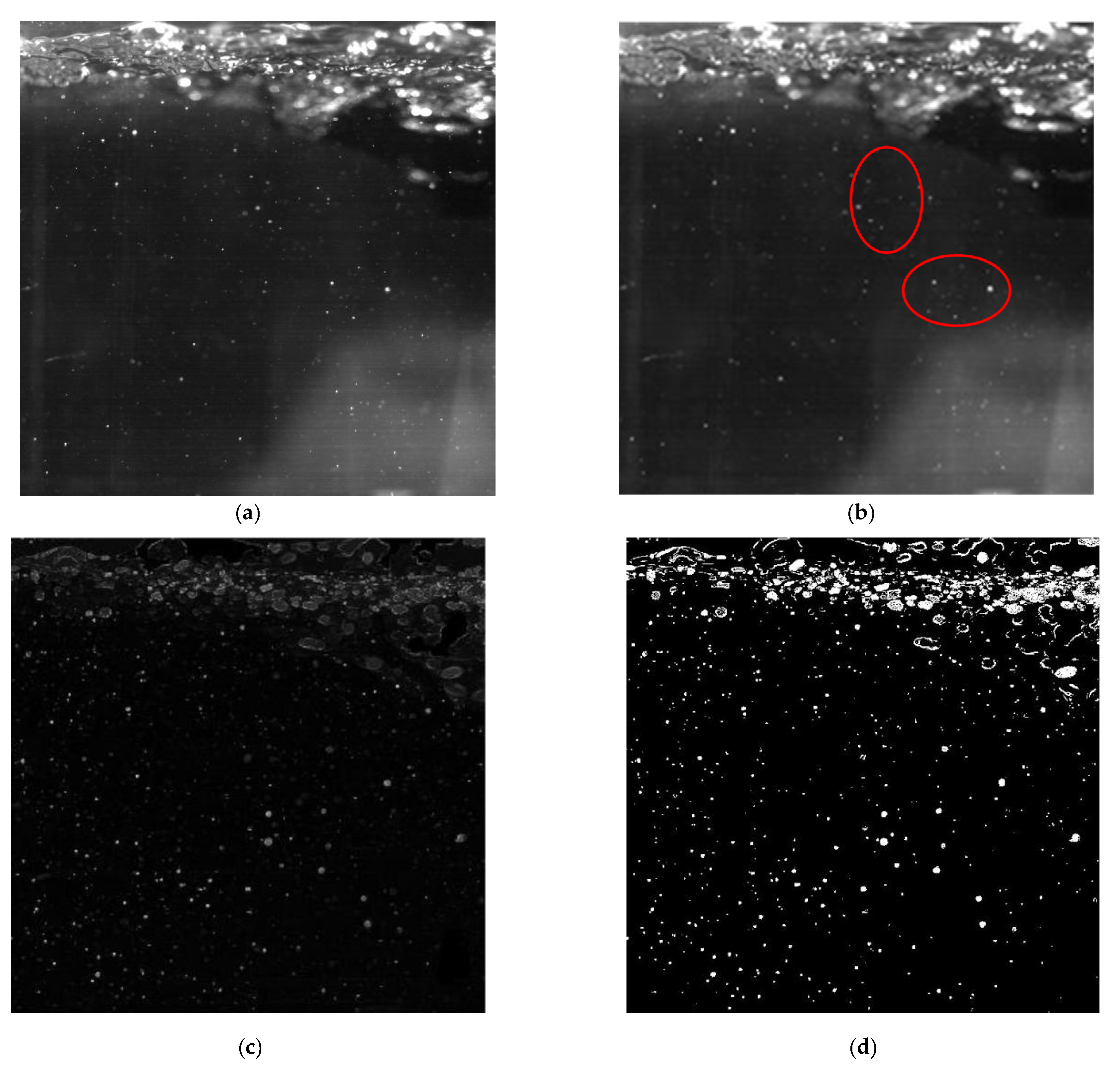
There are some phenomena in the aeration tank, such as overlapping, adhesion, bubble reflection, inconspicuous contrast between bubbles and background and surface reflection of plexiglass, as shown in Figure 4a. Therefore, bubble features are extracted effectively for the original image through MATLAB image processing technology, which includes pre-processing, watershed segmentation, binarization and feature extraction. The process is shown in Figure 4.

3.2.2. Feature Extraction

The feature parameters of bubbles are extracted from the binarization image after pre-processing and watershed segmentation. In order to get the distribution characteristics of bubbles, it is necessary to obtain the position and size of the bubbles.

a.

Bubble position

The coordinates of all pixels of the same bubble are added and averaged, and the average is taken as the coordinates of the bubble. The formulas are as follows:

$$x_c={\displaystyle \sum _{i,j\in \mathsf{\Omega }}\frac{j}{N}}$$

(4)

$$y_c={\displaystyle \sum _{i,j\in \mathsf{\Omega }}\frac{i}{N}}$$

(5)

where, (i, j) represents the pixels of column J in row I of the image, and N is the total number of pixels in the bubble-connected region in the image. Ω denotes the connecting region of the bubble plane.

b.

Bubble size

The moving bubbles are put on unbalanced pressure and deformed, which causes the bubble size to deviate from the experimental size. In order to accurately study the relationship between bubble size and gas–liquid mass transfer, the bubble equivalent diameter, d_b, is introduced. The diameter of a circle with the same area as the elliptical projection is defined as the equivalent diameter of a bubble, as shown in Equation (6):

$${\mathrm{d}}_{\mathrm{b}}=\sqrt{4\mathrm{S}/\mathsf{\pi }}$$

(6)

where, S is the area of the ellipse, m².

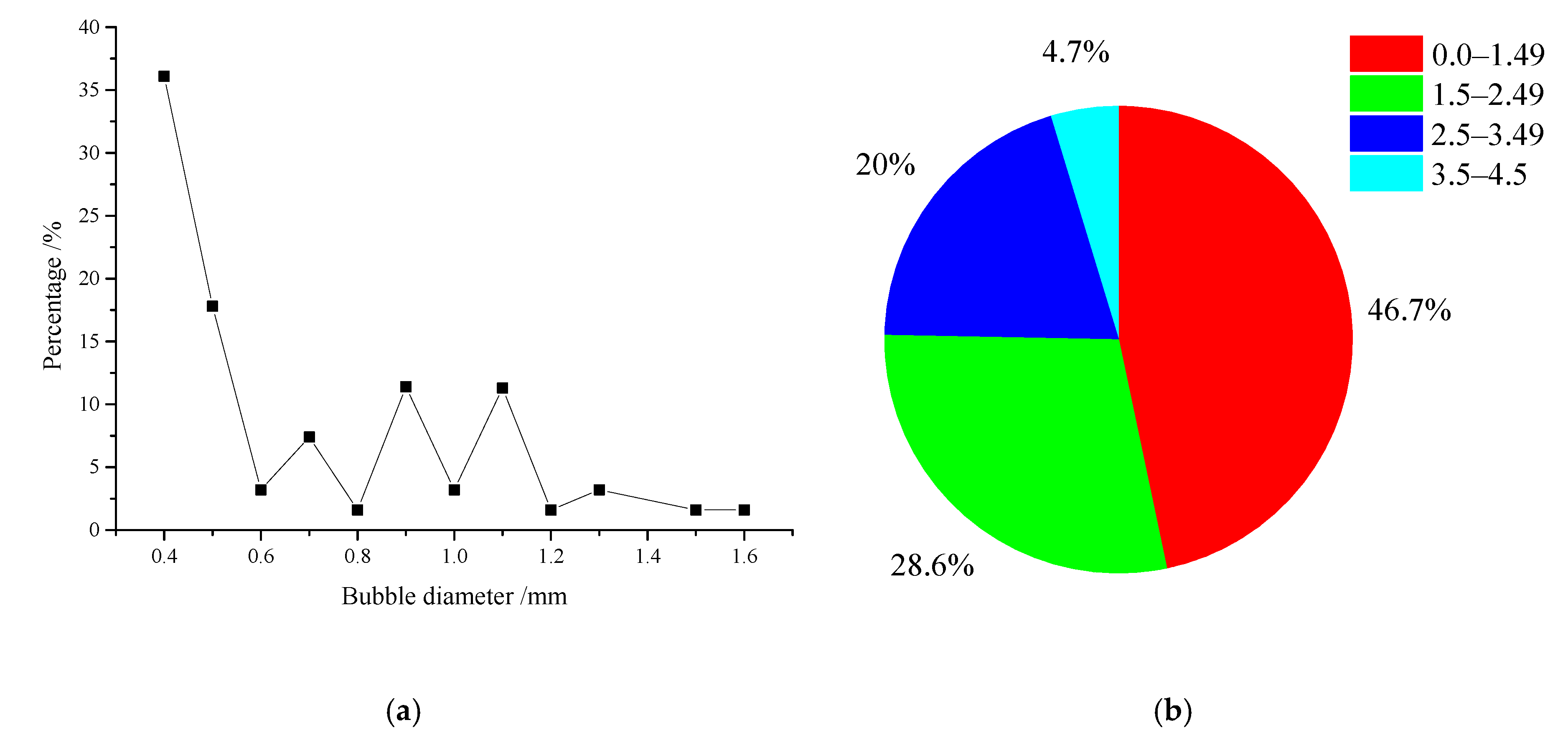
The equivalent diameter of bubbles is calculated according to Equation (5). Figure 5a shows the distribution of bubble diameter. It can be seen from the figure that the bubble size ranges from 0.4 to 1.6 mm, and the number of bubbles varies greatly. Small bubbles with a diameter between 0.4 and 0.6 mm account for a higher proportion of bubbles, reaching 58%. The main reason is that the aeration impeller has a cutting effect on the large bubbles in the process of rotating, and the large bubbles are divided into several small bubbles. For convenience, the bubble diameter in millimeters is converted to pixels. During image processing, the unit pixel is 0.353 mm. So, the bubble size ranges from 0 to 4.5 pixels, the size of bubbles is divided into four categories according to pixels, and the diameters are 0~1.49, 1.5~2.49, 2.5~3.49 and 3.5~4.5 pixels. Figure 5b shows the percentage of bubble size of each group. For the convenience of statistics and simulation, the four kinds of bubble size are rounded, and the diameters are 1, 2, 3 and 4 pixels respectively, and 0.353, 0.71, 1.06 and 1.41 mm respectively, accounting for 46.7%, 28.6%, 20% and 4.7%. The average diameter of the bubbles is about 0.62 mm.

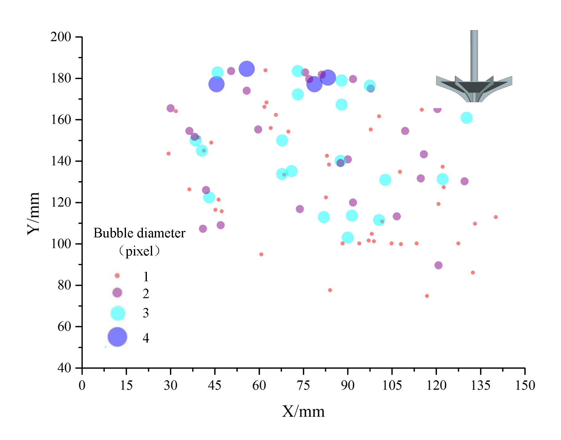
The bubble distribution at an immersion depth of 0 mm and a rotational speed of 250 rpm is shown in Figure 6. The hydraulic jump is more violent under the rotating action of the aeration impeller. A large amount of air enters the liquid and forms bubbles in different sizes due to hydraulic jump and negative pressure entrainment. The bubbles present triangular distribution near the impeller, which appear in not only the upper liquid but also the bottom.

3.2.3. Gas Holdup

The gas holdup is the main parameter that affects the performance of an inverted-umbrella aerator. Therefore, the measurement of gas holdup contributes to the analysis of oxygen mass transfer characteristics of the inverted-umbrella aerator. The liquid level difference method calculates the gas holdup by measuring the difference of liquid level height in the aeration tank during the operation [22,23]. Because of the drastic hydraulic jump, entrainment and other phenomena during the operation of the inverted-umbrella aerator, there are errors in the measurement of liquid level. To accurately obtain the gas holdup, a method is proposed to calculate the gas holdup through high-speed photography and image processing technology. The calculation formula is Equation (7):

$${\mathsf{\alpha }}_{\mathrm{g}}=\frac{{\mathrm{S}}_{\mathrm{bubbles}}}{{\mathrm{S}}_{\mathrm{L}}}$$

(7)

where, S_bubbles is the total area of bubbles, m², and S_L is the total area of gas–liquid two-phase, m².

The gas holdup is 0.0725% at an immersion depth of 0 mm and a rotational speed of 250 r/min.

4. Numerical Calculation Method

4.1. Model and Meshing

The computational domain of the model is divided into two parts: the rotation domain and the static domain. A structured array of hexahedral mesh elements is applied to the model using the Integrated Computer Engineering and Manufacturing code for Computational Fluid Dynamics (ICEM CFD) [24]. The computational domain and mesh are shown in Figure 7. In order to avoid the error of interpolation with different grid sizes of rotor stator interface, the same size of the interface mesh is used. At the same time, the grid size of the interface is locally refined, and the grid size in other computational domains is gradually increased, which can reduce the number of grids and ensure the accuracy of the simulation.

When considering the interaction of aeration and flow driving and gas–liquid two-phase flow, the gas holdup of a certain cross-section in the aeration tank is taken as the grid independence indicator. Six different numbers of grids are selected for the independence test, and the results are shown in

Table 4. The result of grid independence.

	Grid Number		Gas Holdup/%		Relative Error/%
	Static Domain	Rotation Domain	Experiment	Simulation
1	579,000	136,000	0.0769	0.0646	16.0
2	726,000	181,000		0.0692	10.0
3	868,000	226,000		0.0696	9.1
4	1,113,000	272,000		0.07	8.9
5	1,412,000	316,000		0.0695	8.7
6	1,856,000	362,000		0.0703	8.6

. It can be seen from the table that the predicted value of the gas holdup remains unchanged after the grid number is greater than 1.1 × 10⁶. Therefore, the third grid is selected for numerical simulations. Namely, the grid number of the static domain is 8.68 × 10⁵, and the grid number of the rotation domain is 2.26 × 10⁵. The simulation results are less than the experiment results, and the error is about 9.1%. The bubbles with different sections cannot be distinguished in the image processing, which results in the high gas holdup in the experiment.

4.2. Boundary Conditions

FLUENT 15.0 is employed to solve the problem. The process of gas–liquid two-phase flow and dissolved oxygen transport in the aeration tank is an unsteady state. The time step is 0.001 s, and the calculation time is 9 s. The liquid phase is set as the primary phase, and the gas phase is set as the secondary phase. The SIMPLE algorithm is adopted to deal with the pressure-velocity coupling [25]. The first-order upwind scheme is used for volume fraction, turbulent kinetic energy and turbulent dissipation. The gradient of the spatial discretization scheme adopts the least square method based on element volume. Momentum, volume fraction, turbulent kinetic energy and turbulent dissipation all take the first-order windward scheme. The top outlet is set as the pressure outlet [26], the sidewall and the bottom of the aeration tank are set as the no slip wall boundary condition. The impeller is set as a rotational wall. The reference pressure is at 1.01 × 10⁵ Pa, and the gravity acceleration is 9.81 m/s².

4.3. Numerical Calculation Model

The Euler-Euler model is used to simulate the gas–liquid two-phase flow. The drag function uses the Schiller and Naumann model, that is [27]:

$$C_D=\{\begin{array}{ll}24\left(1+0.15R{e}^{0.687}\right)/Re& Re\le 1000\\ 0.44& Re>1000\end{array}$$

(8)

where, $C_D$ is drag coefficient, and Re is relative Reynolds number.

$$Re=\frac{{\rho }_g|u_l-u_g|d_g}{{\mu }_g}$$

(9)

where, ${\rho }_g$ is the volume fraction of gas phase, kg/m³, $u_l$ is velocity of liquid phase, m/s, $u_g$ is velocity of gas phase, m/s, $d_g$ is the diameter of bubbles, m, and ${\mu }_g$ is the dynamic viscosity of gas phase, Pa·s.

Considering the lift generated by the shear and the vortex lift generated by the interaction between the bubbles and the liquid phase, the Moraga lift model, which is more suitable for spherical bubbles, is employed. The governing equation is [28]:

$$F_L=-{\alpha }_g{C}_L{\rho }_l\left(u_g-u_l\right)\times \left(\nabla \times u_l\right)$$

(10)

where, ${\alpha }_g$ is the volume fraction of gas phase, $C_L$ is lift coefficient, ${\rho }_l$ is the volume fraction of liquid phase, kg/m³, $u_g$ is velocity of gas phase, m/s, and $u_l$ is velocity of liquid phase, m/s.

The standard k-epsilon (k–ε) model has good calculation accuracy and efficiency in the calculation of gas–liquid two-phase flow. Therefore, the standard k–ε model is used [12]. k is the turbulent kinetic energy and ε is the turbulent dissipation rate.

Transport equation of k is [27]:

$$\frac{\partial }{\partial t}\left(\rho k\right)+\frac{\partial }{\partial x_i}\left(\rho k{u}_i\right)=\frac{\partial }{\partial x_i}\left[\left(\mu +\frac{{\mu }_l}{{\sigma }_k}\right)\frac{\partial k}{\partial x_i}\right]+G_k+G_b-\rho \epsilon$$

(11)

Transport equation of ε is [27]:

$$\frac{\partial }{\partial t}\left(\rho \epsilon \right)+\frac{\partial }{\partial x_i}\left(\rho \epsilon u_i\right)=\frac{\partial }{\partial x_i}\left[\left(\mu +\frac{{\mu }_l}{{\sigma }_{\epsilon }}\right)\frac{\partial k}{\partial x_i}\right]+C_{1\epsilon }\frac{\epsilon }{k}\left(G_k+C_{3\epsilon }{G}_b\right)-C_{2\epsilon }\rho \frac{{\epsilon }^2}{k}$$

(12)

$${\mu }_l=\rho C_{\mu }\frac{k^2}{\epsilon }$$

(13)

where, G_k is turbulent kinetic energy generated by average velocity gradient, m²/s², G_b is turbulent kinetic energy generated by buoyancy, m²/s², σ_k and σ_ε are prandtl number of k and ε, μ is viscosity coefficient, Pa·s, $\rho$ is arithmetic mean of two-phase density, kg/m³, C_1ε, C_2ε, C_3ε and C_μ are constant, and μ_l is turbulent viscosity, Pa·s.

4.3.1. Two-Fluid Model

The Euler-Euler model is used to simulate the gas–liquid two-phase flow. The Euler-Euler method regards discrete phase and continuous phase as continuous mediums, and at the same time, studies discrete phase and continuous phase motion in the Eulerian coordinate system [25].

(1)

Volume fraction equation:

$${\mathrm{V}}_{\mathrm{q}}={\displaystyle \sum }_{\mathrm{V}}{\mathsf{\alpha }}_{\mathrm{q}}\mathrm{dV}$$

(14)

where, ${\displaystyle \sum }_{\mathrm{q}=1}^{\mathrm{n}}{\mathsf{\alpha }}_{\mathrm{q}}=1$, α_q is the volume fraction of q-phase.

(2)

Mass-conservation equation:

The q-phase continuity equation is:

$$\frac{\partial }{\partial \mathrm{t}}{\mathsf{\alpha }}_{\mathrm{q}}{\mathsf{\rho }}_{\mathrm{q}}+\nabla ·\left({\mathsf{\alpha }}_{\mathrm{q}}{\mathsf{\rho }}_{\mathrm{q}}{\overrightarrow{\mathrm{v}}}_{\mathrm{q}}\right)={\displaystyle \sum }_{\mathrm{p}=1}^{\mathrm{n}}\left({\dot{\mathrm{m}}}_{\mathrm{pq}}-{\dot{\mathrm{m}}}_{\mathrm{pq}}\right)+{\mathrm{S}}_{\mathrm{q}}$$

(15)

where, α_q is the volume fraction of q-phase, ${\mathsf{\rho }}_{\mathrm{q}}$ is the density of q-phase, kg/m³, ${\overrightarrow{\mathrm{v}}}_{\mathrm{q}}$ is current velocity of q-phase, m/s, ${\dot{\mathrm{m}}}_{\mathrm{pq}}$ is mass transfer from p-phase to q-phase, kg, ${\dot{\mathrm{m}}}_{\mathrm{qp}}$ is mass transfer from q-phase to p-phase, kg, generally, ${\mathrm{S}}_{\mathrm{q}}$ = 0.

(3)

Momentum conservation equation:

The q-phase momentum conservation equation is:

$$\begin{array}{c}\frac{\partial }{\partial \mathrm{t}}({\mathsf{\alpha }}_{\mathrm{q}}{\mathsf{\rho }}_{\mathrm{q}}{\overrightarrow{\mathrm{v}}}_{\mathrm{q}})+(\nabla ·{\mathsf{\alpha }}_{\mathrm{q}}{\mathsf{\rho }}_{\mathrm{q}}{\overrightarrow{\mathrm{v}}}_{\mathrm{q}}{\overrightarrow{\mathrm{v}}}_{\mathrm{p}})=-{\mathsf{\alpha }}_{\mathrm{q}}{\nabla }_{\mathrm{q}}+\nabla ·{\overline{\overline{\mathsf{\tau }}}}_{\mathrm{q}}+{\mathsf{\alpha }}_{\mathrm{q}}{\mathsf{\rho }}_{\mathrm{q}}\overrightarrow{\mathrm{g}}\\ +{\displaystyle {\displaystyle \sum }_{\mathrm{p}=1}^{\mathrm{n}}}\left({\overrightarrow{\mathrm{R}}}_{\mathrm{pq}}\left({\overrightarrow{\mathrm{v}}}_{\mathrm{p}}-{\overrightarrow{\mathrm{v}}}_{\mathrm{q}}\right)+{\dot{\mathrm{m}}}_{\mathrm{pq}}{\overrightarrow{\mathrm{v}}}_{\mathrm{pq}}-{\dot{\mathrm{m}}}_{\mathrm{qp}}{\overrightarrow{\mathrm{v}}}_{\mathrm{qp}}\right)\\ +\left({\overrightarrow{\mathrm{F}}}_{\mathrm{q}}+{\overrightarrow{\mathrm{F}}}_{\mathrm{lift},\mathrm{q}}+{\overrightarrow{\mathrm{F}}}_{\mathrm{wl},\mathrm{q}}+{\overrightarrow{\mathrm{F}}}_{\mathrm{vm},\mathrm{q}}+{\overrightarrow{\mathrm{F}}}_{\mathrm{td},\mathrm{q}}\right)\end{array}$$

(16)

where, α_q is the volume fraction of q-phase, ${\mathsf{\rho }}_{\mathrm{q}}$ is the density of q-phase, kg/m³, ${\overrightarrow{\mathrm{v}}}_{\mathrm{q}}$ is current velocity of q-phase, m/s, $\overline{\overline{\mathsf{\tau }}}$ is stress-strain tensor of q-phase, ${\overrightarrow{\mathrm{F}}}_{\mathrm{q}}$ is external volume force, N, ${\overrightarrow{\mathrm{F}}}_{\mathrm{lift},\mathrm{q}}$ is lift, N, ${\overrightarrow{\mathrm{F}}}_{\mathrm{wl},\mathrm{q}}$ is wall slip force, N, ${\overrightarrow{\mathrm{F}}}_{\mathrm{vm},\mathrm{q}}$ is virtual mass force, N, ${\overrightarrow{\mathrm{F}}}_{\mathrm{td},\mathrm{q}}$ is turbulent diffusion force, N, ${\overrightarrow{\mathrm{R}}}_{\mathrm{pq}}$ is interphase force, N, and ${\overrightarrow{\mathrm{v}}}_{\mathrm{pq}}$ is interphase velocity, m/s, which is defined as follows: if ${\dot{\mathrm{m}}}_{\mathrm{pq}}$ > 0, ${\overrightarrow{\mathrm{v}}}_{\mathrm{pq}}$ = ${\overrightarrow{\mathrm{v}}}_{\mathrm{p}}$, if ${\dot{\mathrm{m}}}_{\mathrm{pq}}$ < 0, ${\overrightarrow{\mathrm{v}}}_{\mathrm{pq}}$ = ${\overrightarrow{\mathrm{v}}}_{\mathrm{q}}$, if ${\dot{\mathrm{m}}}_{\mathrm{pq}}$ > 0, ${\overrightarrow{\mathrm{v}}}_{\mathrm{qp}}$ = ${\overrightarrow{\mathrm{v}}}_{\mathrm{q}}$, and if ${\dot{\mathrm{m}}}_{\mathrm{pq}}$ < 0, ${\overrightarrow{\mathrm{v}}}_{\mathrm{qp}}$ = ${\overrightarrow{\mathrm{v}}}_{\mathrm{p}}$.

4.3.2. CFD-PBM Coupled Model

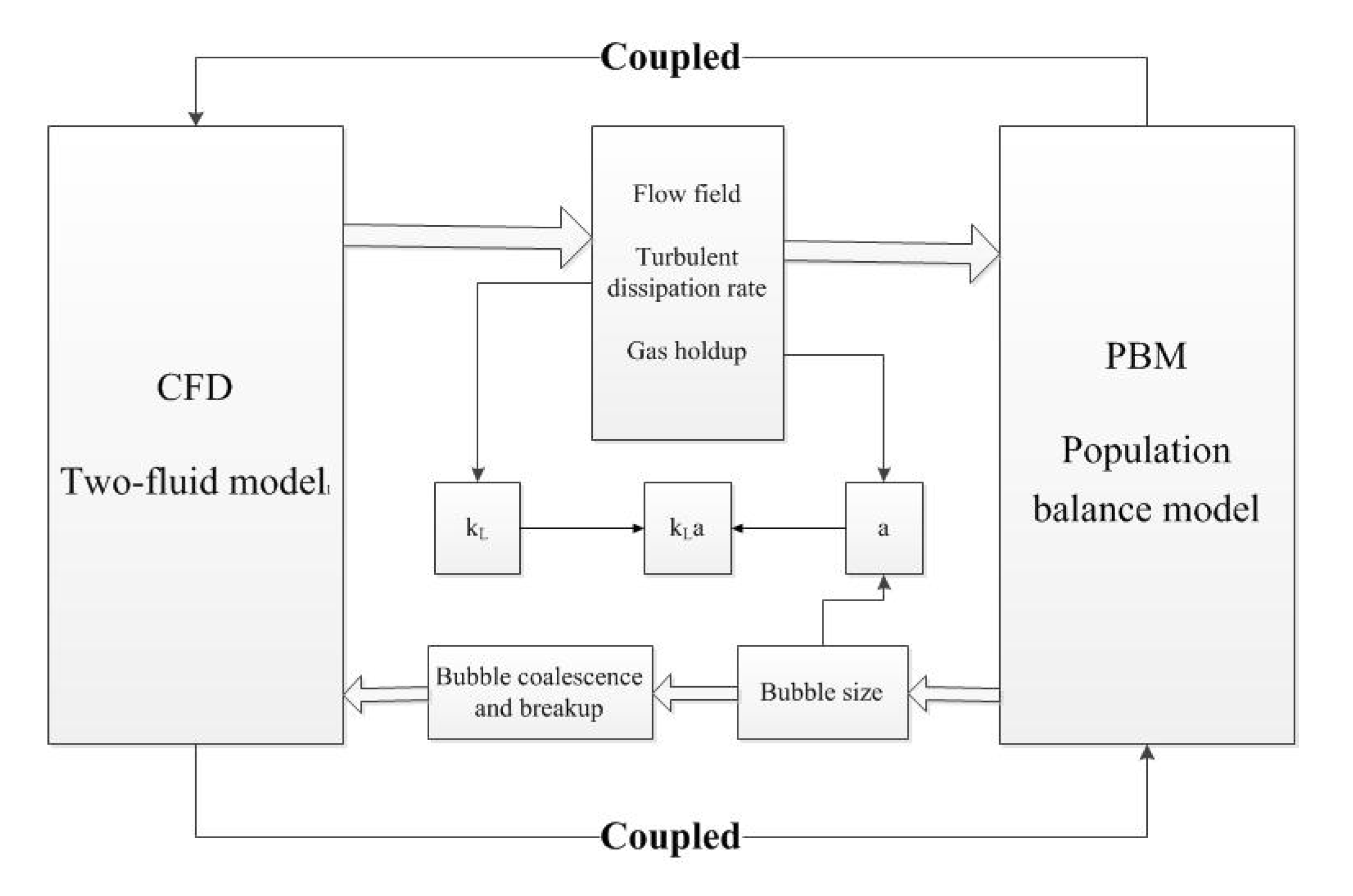
The interaction between bubbles and the bubble coalescence and fragmentation are ignored in the simulation of gas–liquid two-phase flow with a single bubble size. It cannot accurately describe the real flow in the aeration tank [29]. In order to better study the effect of bubble size on gas–liquid flow in the aeration tank, the CFD coupled population balance model (PBM) is employed in this paper. Figure 8 shows the diagram of the CFD-PBM coupled model. The flow field, gas holdup and turbulent energy dissipation rate are calculated by CFD and used to solve PBM [19]. The bubble size distribution obtained from the experiment is input into PBM, which considers bubble coalescence and breakup.

PBM is a standard method to describe the size distribution of the dispersed phase in multiphase flow simulation. The Luo-model, which considers bubble coalescence and fragmentation, is coupled, and it can adequately reflect the gas–liquid two-phase flow in the aeration tank. The population balance equation is expressed as [17]:

$$\begin{array}{l}\frac{\partial n\left(v,t\right)}{\partial t}+\nabla \left[u_{b}n\left(v,t\right)\right]=\frac{1}{2}{\displaystyle {\int }_0^{v}a\left(v-v^{\prime },v^{\prime }\right)}n\left(v-v^{\prime },t\right)d{v}^{\prime }\\ -{\displaystyle {\int }_0^{\infty }a\left(v,v^{\prime }\right)n\left(v,t\right)n\left(v^{\prime },t\right)d{v}^{\prime }+{\displaystyle {\int }_{\mathsf{\Omega }}vb\left(v^{\prime }\right)\beta \left(v|v^{\prime }\right)n\left(v^{\prime },t\right)d{v}^{\prime }-b\left(v\right)n\left(v,t\right)}}\end{array}$$

(17)

where, n(v,t) is the bubble size distribution function, a(v,v’) is the bubble coalescence rate function, b(v) is the bubble fragmentation rate function and β(v|v’) is the probability density function of the sub bubbles generated by the bubble fragmentation from v to v’.

The rate of coalescence and breakup can be expressed as [30]:

$${\mathsf{\phi }}_{\mathrm{n}}^{\mathrm{RC}}=-{\mathrm{C}}_{\mathrm{RC}1}\frac{{\mathsf{\alpha }}_{\mathrm{g}}^2{\mathsf{\epsilon }}^{1/3}}{{\mathrm{D}}_{\mathrm{s}}^{11/3}}\times \frac{\exp \left(-{\mathrm{C}}_{\mathrm{RC}2}\sqrt{\mathrm{We}/{\mathrm{We}}_{\mathrm{cr}}}\right)}{\left({\mathsf{\alpha }}_{\max }^{1/3}-{\mathsf{\alpha }}_{\mathrm{g}}\right)/{\mathsf{\alpha }}_{\mathrm{g}}^{1/3}+{\mathrm{C}}_{\mathrm{RC}3}{\mathsf{\alpha }}_{\mathrm{g}}\sqrt{\mathrm{We}/{\mathrm{We}}_{\mathrm{cr}}}}$$

(18)

$${\mathsf{\phi }}_{\mathrm{n}}^{\mathrm{TI}}=-{\mathrm{C}}_{\mathrm{TI}1}\frac{{\mathsf{\alpha }}_{\mathrm{g}}\left(1-{\mathsf{\alpha }}_{\mathrm{g}}\right){\mathsf{\epsilon }}^{1/3}}{{\mathrm{D}}_{\mathrm{s}}^{11/3}}\frac{\exp \left(-{\mathrm{We}}_{\mathrm{cr}}/\mathrm{We}\right)}{1+{\mathrm{C}}_{\mathrm{TI}2}\left(1-{\mathsf{\alpha }}_{\mathrm{g}}\right)\sqrt{\mathrm{We}/{\mathrm{We}}_{\mathrm{cr}}}}$$

(19)

where, C_RC is coalescence model constant, C_RC1 = 2.86, C_RC2 = 1.017, C_RC3 = 1.922. C_TI is rupture model constant, C_TI1 = 1.6, C_TI2 = 0.42. We_cr is critical Weber for bubble fragmentation, W_ecr = 1.42, and α_max is critical gas holdup, α_max = 0.52.

In order to simulate the flow field and mass transfer coefficient in the aeration tank more accurately, the bubble diameter and proportion are determined by high-speed photography experimental results, and PBM is employed. A single bubble size of 0.62 mm (average diameter) is set as the control group.

5. Results and Discussion of Gas–liquid Two-Phase Flow Considering Bubble Size

5.1. Results and Discussion of the Gas–Liquid Two-Phase Flow Field

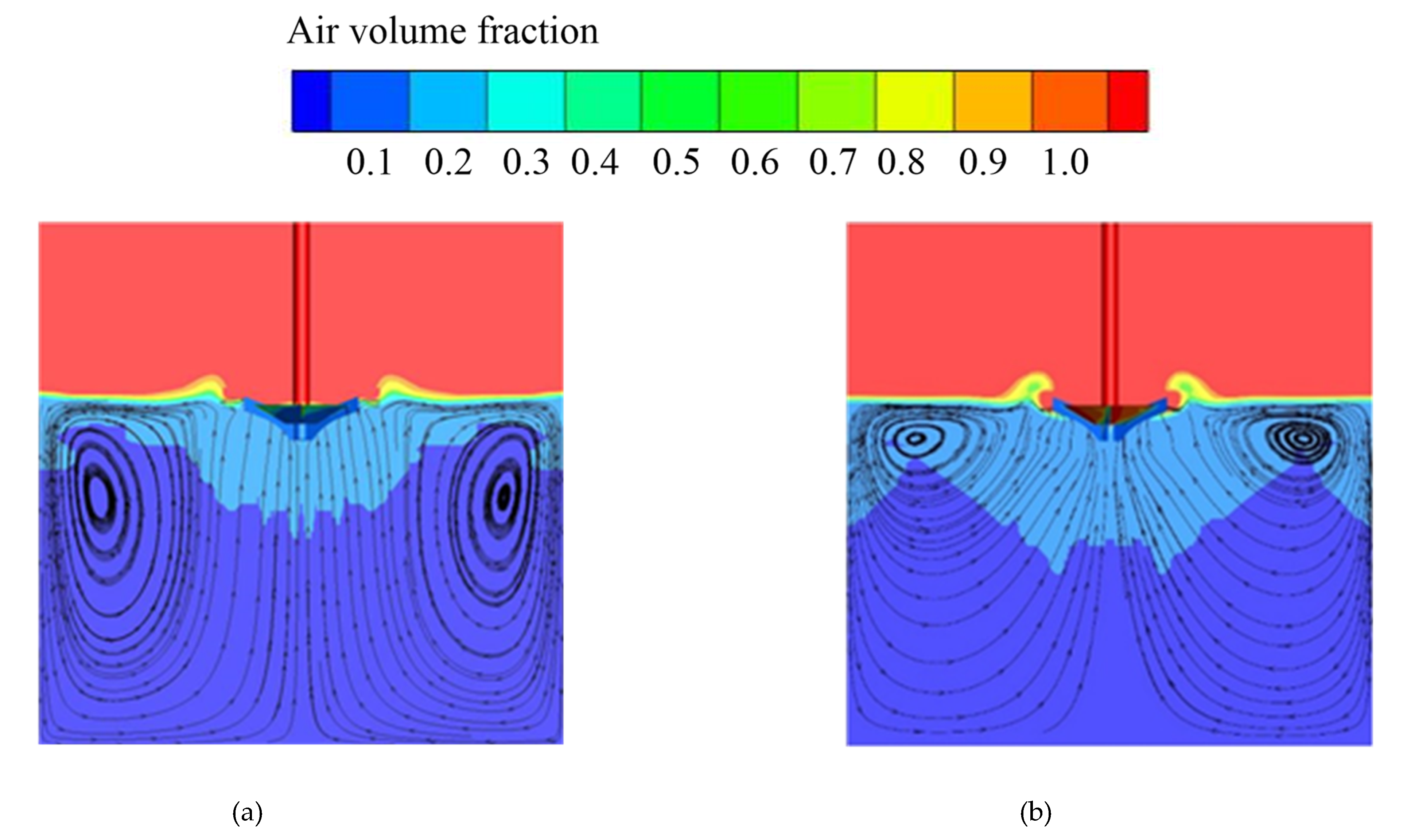
The gas–liquid two-phase distribution in the aeration tank is studied, and the flow field is shown in Figure 9.

It can be seen from the figure that the fluid under the liquid level on the left and right sides has the same flow law in the process of impeller rotation, which is approximately symmetrical distribution. The liquid diffuses longitudinally all around, and a small part of the liquid is impacted by the wall to form reflux after reaching the wall. The rest of the liquid moves along the wall to the bottom. The bottom fluid is lifted to the impeller by the lift of inverted-umbrella aerator, and the circumfluence vortex appears. The circumfluence vortex accelerates the exchange of liquid between the shallow layer and bottom layer, and the renewal of liquid is accelerated.

It can also be seen from the figure that the circulation vortices under the average diameter scheme and PBM scheme are different. As a surface aerator, the inverted-umbrella aerator mainly affects the shallow liquid, so the circulation vortex should be close to the free surface. Also, the gas–liquid interface is clear in most areas of the aeration tank, and there is a clear entrainment above the impeller. The gas phase first appears in shallow liquid due to the negative pressure entrainment. With the influence of the circulation vortex, it gradually moves to the bottom to complete the gas–liquid mixing. In conclusion, PBM can accurately simulate the gas–liquid two-phase flow distribution in the aeration tank.

5.2. Results and Discussion of Mass Transfer Coefficient

The oxygen mass transfer coefficient, k_La, includes two parameters: the liquid-phase mass transfer coefficient, k_L, and the interfacial area, a (the total area of interface between bubbles and liquid). The gas–liquid two-phase flow in the aeration tank is explained from the above two parameters.

a.

Liquid-phase mass transfer coefficient

k_L is calculated as follows [31]:

$${\mathrm{k}}_{\mathrm{L}}=\mathrm{c}{\left({\mathrm{D}}_{\mathrm{L}}\right)}^{1/2}{\left(\frac{\mathsf{\epsilon }\mathsf{\rho }}{\mathsf{\mu }}\right)}^{1/4}$$

(20)

where, D_L is diffusivity on the liquid, m²/s, ε is turbulent dissipation rate, w/kg, ρ is liquid density, kg/m³, μ is dynamic viscosity, Pa·s, and C is correction coefficient, taken as 1.13.

In order to determine k_L, the turbulent dissipation rate, ε, needs to be estimated, and ε is calculated as follows [31]:

$$\epsilon ={\epsilon }_{ave}=\frac{P}{\rho \left(\pi /4\right)T^{2}H}$$

(21)

where, ε_ave is average value of turbulent dissipation rate, w/kg, P is power input under gassed conditions, W, $\rho$ is liquid density, kg/m³, T is impeller diameter, m, and H is blade height of impeller, m.

k_L varies with the change of turbulent dissipation rate, which is different at different positions. Therefore, the turbulent dissipation rate is solved by the volume average method in post-processing, and the liquid-phase mass transfer coefficient, k_L, is calculated.

b.

Interfacial area

a is calculated as follows:

$$a=\frac{6{\alpha }_g}{d_b}$$

(22)

where, α_g is gas holdup, %, and d_b is bubble equivalent diameter, m.

5.2.1. Results and Discussion of Liquid-Phase Mass Transfer Coefficient

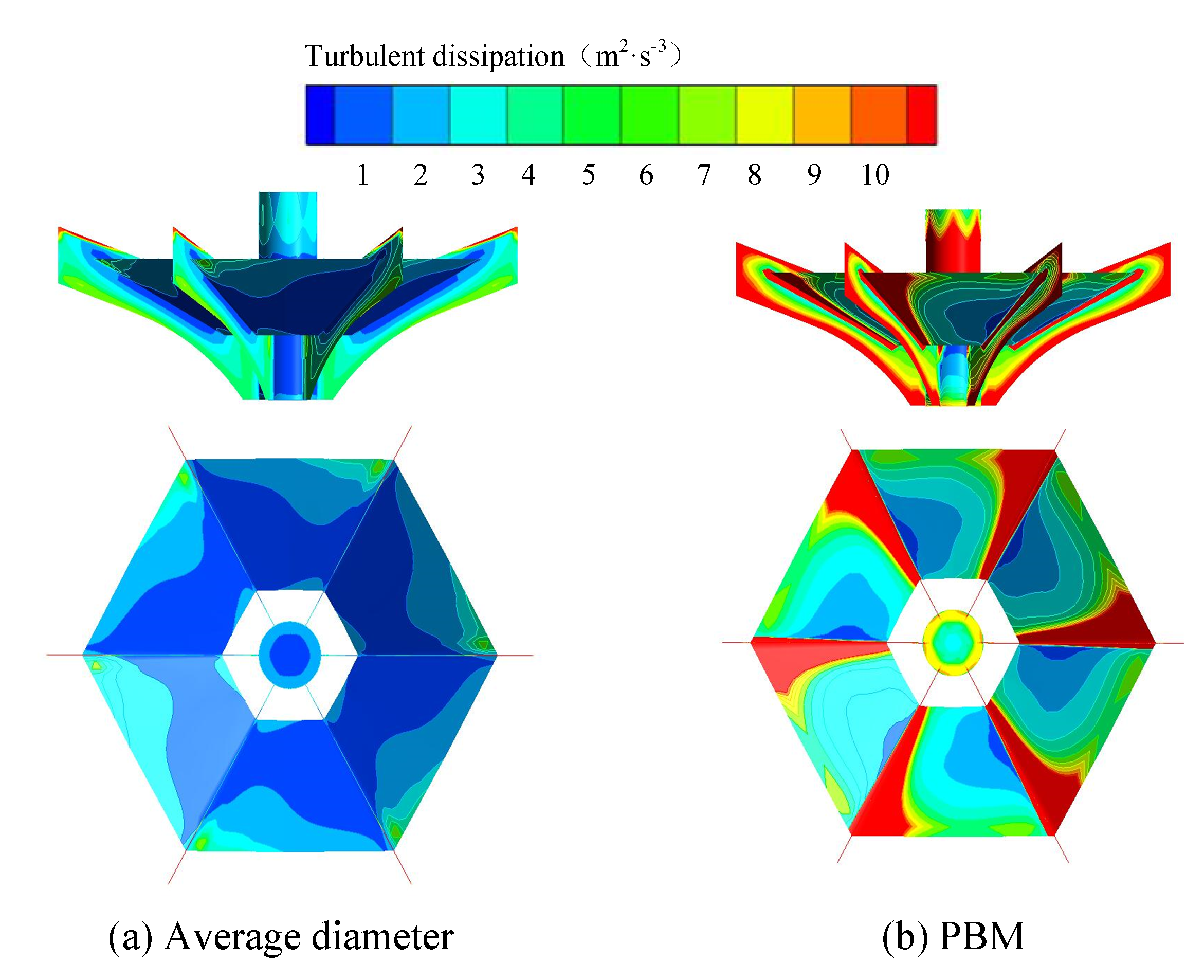
It can be seen from Equation (20) that the turbulent dissipation rate is the main parameter affecting the variation of k_L. So, it is necessary to analyze the turbulence dissipation rate. The turbulent dissipation rate is the rate at which mechanical energy is converted into heat energy, and most of them occur in the fluid–solid contact area. Therefore, the impeller of the inverted-umbrella aerator is selected to analyze the turbulent dissipation rate.

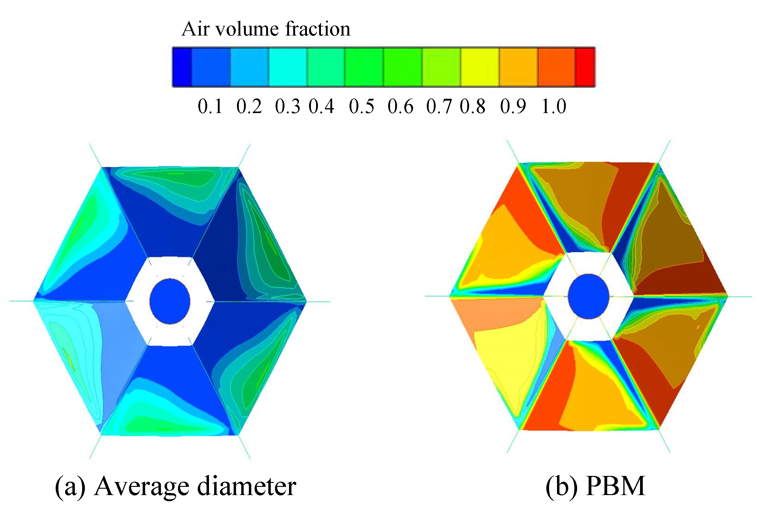
The distribution of air volume fraction and turbulent dissipation rate is shown in Figure 10 and Figure 11.

It can be seen from the figures that the air volume fraction on the upper side of the plate in the PBM scheme is significantly higher than in the average diameter scheme, and a high air concentration area is formed on the top side of the plate. The air is more likely to diffuse under the concentration gradient, which shows that the gas transportation capacity is great. The air volume fraction on the back of the blade decreases with the increase of bubble size, which hinders air diffusion. The turbulent dissipation rate is mainly concentrated in the edge of the blade and the region with high air volume fraction. The average turbulent dissipation rate of the average diameter scheme and the PBM scheme is 0.28 and 0.63, respectively.

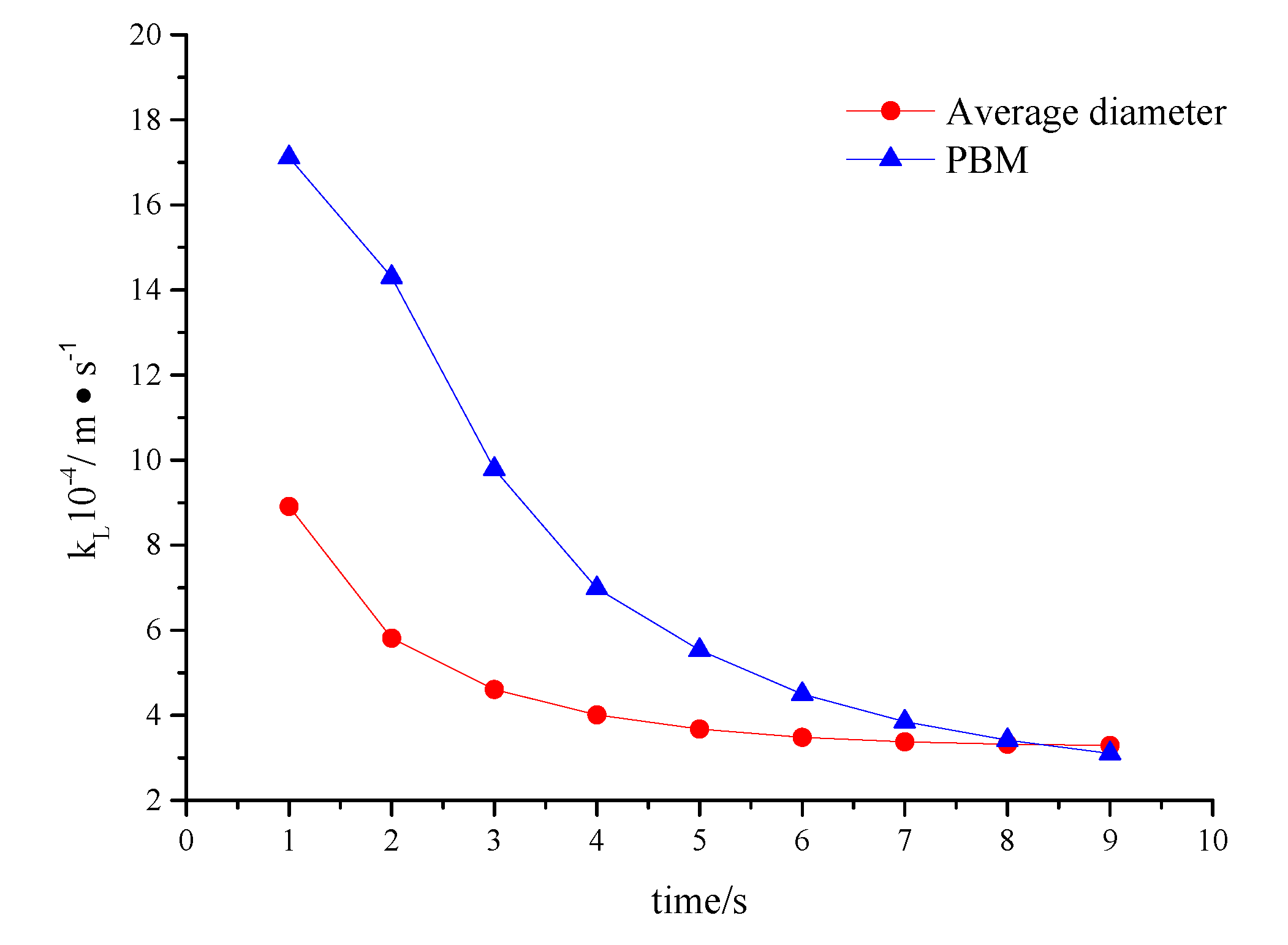
The variation of liquid-phase mass transfer coefficient, k_L, is shown in Figure 12. The liquid-phase mass transfer coefficient, k_L, decreases rapidly during 0~6 s, and it is stable at 6 s. The variation of k_L tends to be smooth and keeps at about 4 × 10⁻⁴ m·s⁻¹. The concentration gradient on both sides of the gas–liquid two-film is the largest at the beginning, the resistance when the gas enters liquid through the liquid membrane is the smallest, and liquid-phase mass transfer coefficient is more substantial. Bubble transfer and mass transfer appear in liquid with the increase of calculation time due to hydraulic jump and entrainment. The concentration difference between the two sides of the gas–liquid two-film decreases, and liquid-phase mass transfer coefficient decreases. Liquid-phase mass transfer coefficient of the PBM scheme is higher than the average diameter scheme. Bubble coalescence occurs in the PBM scheme, which leads to the increase of bubble size, and the retention time of bubbles in liquid is shortened. The total mass transfer is reduced at the same time, resulting in a higher concentration difference.

In conclusion, the bubble size affects the turbulent dissipation rate of the aerator, and indirectly affects the liquid-phase mass transfer coefficient, k_L. However, the order of the liquid-phase mass transfer coefficient is small, and it needs to be 1/4 square root through the turbulent dissipation rate. Therefore, the variation of liquid-phase mass transfer coefficient with different bubble sizes is not apparent. It is necessary to study the interfacial area.

5.2.2. Results and Discussion of Interfacial Area

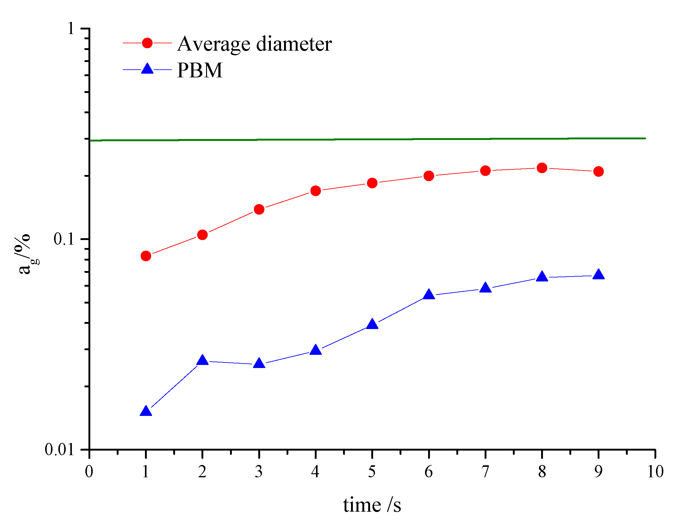
The variation of gas holdup is shown in Figure 13. The green line in the figure is the gas holdup test value at oxygen saturation under the same working condition (the rotational speed is 250 r/min, and immersion depth is 0 mm).

As can be seen from the figure, the gas holdup increases during 0~7 s and the curves change smoothly and tend to be stable in 7~9 s. The gas holdup in the PBM scheme is much smaller than in the average diameter scheme under the same calculation time, which is closer to the test. The main reason is that bubble coalescence is considered in the PBM scheme. The bubble coalescence will cause an increase in bubble size. Bubbles stay a short time in the liquid, and the overall gas holdup is reduced. The deviation between the simulated value and test value of gas holdup is about 7.2% in a stable state, which is within the normal range. The results show that PBM has good applicability in the simulation of gas–liquid two-phase flow which involves bubble mass transfer.

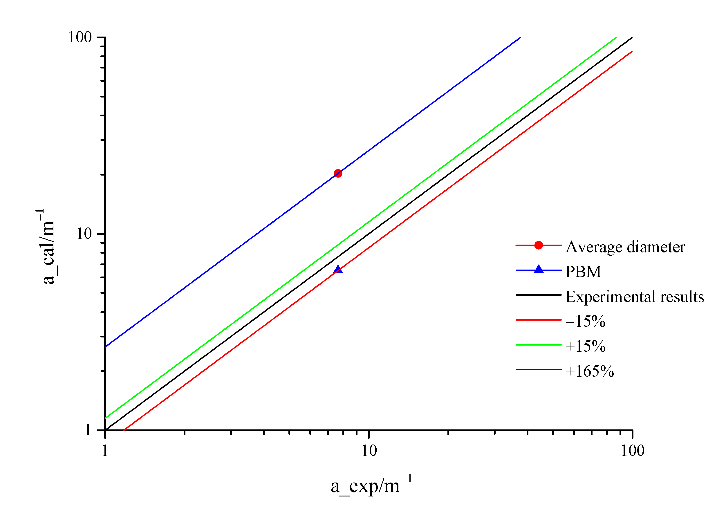
The interfacial area, when it is stable, is shown in Figure 14. It can be seen from the figure that the interfacial area is directly related to the bubble size in a steady state. The interfacial area in the PBM scheme is much smaller than in the average diameter scheme, and it is closer to the test value, with a relative deviation of about 12%. This is because the bubble coalescence is considered in PBM, which results in large-scale bubbles. The bubble number is smaller than in the average diameter scheme after coalescence. Large size bubbles move to the free surface after coalescence, which causes the waves of the free surface to break. The contact area between the liquid and gas is increased and free surface mass transfer is strengthened, but the bubble mass transfer is still dominant. Therefore, the interfacial area is smaller when the bubble size varies (in the PBM scheme), and the area is 6.51 m⁻¹.

5.2.3. Results and Discussion of Standard Oxygen Mass Transfer Coefficient

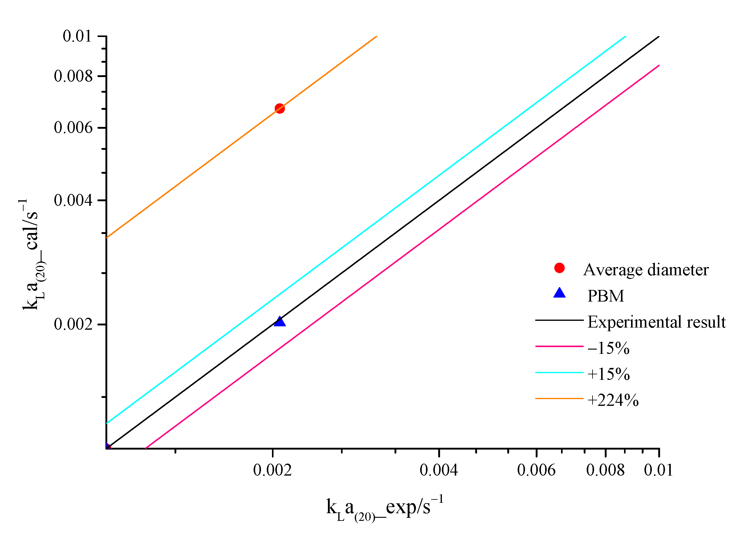
The comparison of standard oxygen mass transfer coefficient in stable state is shown in Figure 15. It can be seen from the figure that the calculation precision of the PBM scheme is higher, and the deviation is less than 3%, which is similar to the test value. The simulation value of the average diameter scheme is much greater than the test value. It shows that the CFD-PBM coupled model can improve the accuracy of calculation results in the simulation of gas–liquid two-phase flow.

6. Conclusions

In this paper, the aeration performance and the internal flow in the aeration tank were studied by both experimental and numerical simulations with the CFD-PBM coupled model when the immersion depth of the inverted-umbrella aerator impeller was 0 mm and the rotational speed of the impeller was 250 r/min. The main conclusions are as follows:

(1)

The size of bubbles in the aeration tank was different at an immersion depth of 0 mm and a rotational speed of 250 r/min, ranging from 0.4 to 1.6 mm.

(2)

The CFD-PBM coupled model can be considered as the effect of real bubble breakup and coalescence. Compared with the Euler-Euler two-fluid model with a single particle size, it can better simulate the gas–liquid two-phase flow field in the aeration tank.

(3)

The calculation precision of the liquid-phase mass transfer coefficient, k_L, interfacial area, a, and standard oxygen mass transfer coefficient, k_La, of the PBM scheme was higher than the average diameter scheme. The CFD-PBM coupled model can improve the accuracy of calculation, resulting in the simulation of gas–liquid two-phase flow.

References

- Dong, L.; Wang, Y.; Dai, C.; Liu, H.; Ming, J. Prediction of aeration performance for inverted umbrella aerator based on dimensional analysis. J. Chem. Eng. Jpn. 2019, 52, 369–376. [Google Scholar] [CrossRef]
- Fayolle, Y.; Cockx, A.; Gillot, S.; Roustan, M.; Heduit, A. Oxygen transfer prediction in aeration tanks using CFD. Chem. Eng. Sci. 2007, 62, 7163–7171. [Google Scholar] [CrossRef]
- Burgess, J.M.; Calderbank, P.H. The measurement of bubble parameters in Two-Phase dispersions—I: The development of an improved probe technique. Chem. Eng. Sci. 1975, 30, 743–750. [Google Scholar] [CrossRef]
- Burgess, J.M.; Calderbank, P.H. The measurement of bubble properties in two-phase dispersions—III: Bubble properties in a freely bubbling Fluidised-Bed. Chem. Eng. Sci. 1975, 30, 1511–1518. [Google Scholar] [CrossRef]
- Liu, J.W. Gas-Liquid Flow Mechanism and Optimization Design Research for Inverted Umbrella Aerator. Master’s Thesis, Jiangsu University, Zhenjiang, China, 2019. [Google Scholar]
- Lee, W.H.; Lee, J.-H.; Bishop, P.L.; Papautsky, I. Biological application of Micro-Electro mechanical systems microelectrode array sensors for direct measurement of phosphate in the enhanced biological phosphorous removal process. Water Environ. Res. 2009, 81, 748–754. [Google Scholar] [CrossRef] [PubMed]
- Xing, C.; Wang, T.; Wang, J. Experimental study and numerical simulation with a coupled CFD–PBM model of the effect of liquid viscosity in a bubble column. Chem. Eng. Sci. 2013, 95, 313–322. [Google Scholar] [CrossRef]
- Dhotre, M.; Niceno, B.; Smith, B. Large eddy simulation of a bubble column using dynamic Sub-Grid scale model. Chem. Eng. J. 2008, 136, 337–348. [Google Scholar] [CrossRef]
- Milelli, M.; Smith, B.L.; Lakehal, D. Large-Eddy Simulation of Turbulent Shear Flows Laden with Bubbles. Mech. Eng. Cong. Exp. 2001, 8, 461–470. [Google Scholar]
- Deen, N.G.; Solberg, T.; Hjertager, B. Large eddy simulation of the Gas–Liquid flow in a square cross-sectioned bubble column. Chem. Eng. Sci. 2001, 56, 6341–6349. [Google Scholar] [CrossRef]
- Dong, L.; Liu, J.; Liu, H.; Dai, C.; Gradov, D.V. Study on the internal Two-Phase flow of the Inverted-Umbrella aerator. Adv. Mech. Eng. 2019, 11, 1–13. [Google Scholar] [CrossRef]
- Karpinska, A.M.; Bridgeman, J. CFD-Aided modelling of activated sludge Systems—A critical review. Water Res. 2016, 88, 861–879. [Google Scholar] [CrossRef] [PubMed] [Green Version]
- Zhang, X.K.; Yao, T. CFD analysis seawater treatment plant for Flue Gas Desulphurization (FGD). Power Eng. 2004, 24, 276–279. [Google Scholar]
- Lehr, F.; Millies, M.; Mewes, D. Bubble-Size distributions and flow fields in bubble columns. AIChE J. 2002, 48, 2426–2443. [Google Scholar] [CrossRef]
- Buwa, V.V.; Ranade, V.V. Characterization of dynamics of Gas-Liquid flows in rectangular bubble columns. AIChE J. 2004, 50, 2394–2407. [Google Scholar] [CrossRef]
- Gupta, A.; Roy, S. Euler–Euler simulation of bubbly flow in a rectangular bubble column: Experimental validation with Radioactive Particle Tracking. Chem. Eng. J. 2013, 225, 818–836. [Google Scholar] [CrossRef]
- Xu, Y.; Dong, H.F.; Tian, X.; Zhang, X.P.; Zhang, S.J. CFD-PBM coupled simulation of ionic Liquid-Air Two-Phase flow in bubble column. J. Chem. Ind. Eng. 2011, 62, 2699–2706. [Google Scholar]
- Wang, L.; Su, J.W.; Zhang, X.P.; Yang, S. Numerical simulation of Gas-Liquid Two-Phase flow at variousinlet positions in bubble column at low gas velocity. J. Southwest Jiaotong Univ. 2018, 53, 164–172. [Google Scholar]
- Wang, T.; Wang, J. Numerical simulations of Gas–Liquid mass transfer in bubble columns with a CFD–PBM coupled model. Chem. Eng. Sci. 2007, 62, 7107–7118. [Google Scholar] [CrossRef]
- Wang, T. Simulation of bubble column reactors using CFD coupled with a population balance model. Front. Chem. Sci. Eng. 2010, 5, 162–172. [Google Scholar] [CrossRef]
- Inverted-Umbrella Type Surface Aerator; Standards Press of China: Beijing, China, 2014; pp. 10–11.
- De Jesus, S.S.; Neto, J.M.; Santana, A.; Filho, R. Influence of impeller type on hydrodynamics and Gas-Liquid Mass-Transfer in stirred airlift bioreactor. AIChE J. 2015, 61, 3159–3171. [Google Scholar] [CrossRef]
- De Jesus, S.S.; Neto, J.M.; Filho, R. Hydrodynamics and mass transfer in bubble column, conventional airlift, stirred airlift and stirred tank bioreactors, using viscous fluid: A comparative study. Biochem. Eng. J. 2017, 118, 70–81. [Google Scholar] [CrossRef]
- Liu, L.G. Flow Simulation and Optimization Research of Oxidation Ditch with Fine Bubble Based on CFD-PBM Coupled Model. Master’s Thesis, Shanxi Agricultural University, Ya’an, China, 2017. [Google Scholar]
- Guo, Y.Y. Numerical Simulation of the Effect of Radius of Impeller and Its Installation Deptht on the Gas-Liquid Two-Phase Flow in a Stirred Tank. Master’s Thesis, Xi’an University of Technology, Xi’an, China, 2018. [Google Scholar]
- Karpinska, A.M.; Bridgeman, J. Towards a robust CFD model for aeration tanks for sewage Treatment—A Lab-Scale study. Eng. Appl. Comput. Fluid Mech. 2017, 11, 371–395. [Google Scholar] [CrossRef]
- Xiao, H.F. CFD Numerical Simulation of Gas-Liquid Flow in Aeration Tank. Master′s Thesis, Dong Hua University, Shanghai, China, 2010. [Google Scholar]
- Zhang, X.; Peng, J.M.; Cong, J.L.; Li, X.J.; Chen, Y.Y. Uncertainty analysis on boundary condition in subcooled boiling flow by deterministic sampling. Atom. Energy Sci. 2019, in press. [Google Scholar]
- Zhang, B. Numercial Simulation of Gas-Liquid Flow in a Pressurized Bubble Column Using the CFD-PBM Coupled Model. Master’s Thesis, Beijing Institute of Petrochemical Technology, Beijing, China, 2018. [Google Scholar]
- Duan, X.Y.; Zhang, Z.B.; Li, Y.Z.; Tu, J.Y. Simulation of Flowing Characteristics in Complex Bubbly Flow with Population Balance Model. J. Chem. Ind. Eng. 2011, 62, 928–933. [Google Scholar]
- Garcia-Ochoa, F.; Gomez, E. Theoretical prediction of Gas–Liquid mass transfer coefficient, specific area and Hold-Up in sparged stirred tanks. Chem. Eng. Sci. 2004, 59, 2489–2501. [Google Scholar] [CrossRef]
Figure 1.
The geometric parameters of the impeller.
Figure 2.
Schematic diagram of the test system.
Figure 3.
Dissolved oxygen concentration curve and fitting results.
Figure 4.
Image processing process. (a) Original image, (b) nonlinear smoothing filtering, (c) watershed image after segmentation, (d) binarization image.
Figure 5.
Bubble size distribution. (a) Bubble diameter distribution, (b) percentage of bubble size of each group.
Figure 6.
Bubble distribution.
Figure 7.
Computational domain and mesh. (a) Computational domain, (b) mesh generation, (c) mesh of the impeller.
Figure 8.
The diagram of the computational fluid dynamics-population balance model (CFD-PBM) coupled model.
Figure 9.
Gas–liquid two-phase distribution in aeration tank. (a) Average diameter, (b) PBM.
Figure 10.
Distribution of air volume fraction. (a) Average diameter, (b) PBM.
Figure 11.
Distribution of turbulent dissipation rate. (a) Average diameter, (b) PBM.
Figure 12.
Variation of kL in different schemes.
Figure 13.
Variation of gas holdup.
Figure 14.
Comparison of interfacial area.
Figure 15.
Comparison of standard oxygen mass transfer coefficient.