Stereo Particle Image Velocimetry Measurements of the Wake Fields Behind A Panamax Bulker Ship Model Under the Ballast Condition

Abstract

Particle image velocimetry is applied in this study to measure the wake flow field of a Panamax Bulker ship model under the ballast condition. This investigation revealed that the Froude number is 0.167. The time-averaged velocity, turbulent fluctuations, turbulent kinetic energy (TKE), Reynolds stresses, and vorticity information were measured to perform a comparison with the design condition. The time-averaged velocity contours indicated that the ballast and design conditions have distinct hook-like axial velocity contours; however, they appeared at different positions. The big difference under the ballast condition is that the top of the propeller disk area is near the free surface and a region with strong root mean square velocity fluctuation is formed near the free surface. The TKE, the Reynolds stresses, and the hub cap vortex (Hcv) are all affected by the turbulent velocity fluctuation region under the ballast condition. A strong bilge vortex (Bv) is produced when the water flows through the U-shaped stern for the design and ballast conditions.

1. Introduction

Bulk carriers, oil tankers, and container ships are three main types of ships and they occupy a very important position in the international shipping industry. As of 1 January 2018, there are more than 94,171 merchant ships that totals almost 1.92 billion dead weight tons (DWT). Of these, 42.5% are bulk carriers, 29.2% are oil tankers, and 13.1% are container ships [1]. By having detailed measurements combined with an accurate knowledge and an insight into the flow characteristics of ships, this forms the basis for the theory and numerical simulations verification of the hull optimization and the propeller design.

The particle image velocimetry (PIV) method has an extensive use on measuring the wake of ships and propellers. Due to the coupled interaction of the turbulent boundary layer, 3D flow separation, and the orbital motion of water particles, the flow characteristics around the ships are very complex [2,3]. In addition, the flow characteristics are affected by the hull form, stern type, and loading conditions. For bulk carriers, the ballast condition accounts for almost 50% of the total operation time [4]. Our previous paper [2] described in detail the measurement of the wake fields based on the PIV under the design-loading condition, and most of the literature focuses on the flow characteristics around the hulls under the design conditions [5,6,7,8,9,10,11,12,13]. The flow characteristics around the ship under the ballast condition is different from that under the design condition with the change in the draft, inclination angle, and the float status. Hence, the literature review of this paper focuses on the hydrodynamic performance, especially the flow field measurement, for the ballast conditions.

Lee et al. [3] applied a 2D-PIV system to study the wake field of a Korea Research Institute of Ships & Ocean engineering (KRISO) container ship (KCS) with Lpp = 1.422 m under the design and ballast conditions in a circulating water channel. The PIV measurement results show that the intensity of the longitudinal counter-rotating vortices and the location of the vortex core are significantly different under the two conditions. Wu et al. [14,15] used the LaVision underwater stereoscopic particle image velocimetry (SPIV) system to measure the phase averaged wake fields in the wave of the second variant of KRISO very large crude carrier (KVLCC2) hull under the design and ballast conditions. At the same time, the corresponding numerical study was carried out using computational fluid dynamics (CFD) Ship-Iowa V4.5 code. The experimental and numerical results show that the ballast condition has a different axial velocity distribution, a hook-shaped velocity contour, and vortex distribution characteristics under the design condition. Park et al. [4] applied experimental and numerical methods to study the added resistance in the wave under the full-load, ballast, and two intermediate conditions. Luo et al. [16] conducted a numerical study on the viscous flow field around a KCS ship with Lpp = 7.2786 m under the ballast conditions. The influence of the different loading conditions on the surrounding flow field of the ship is described by the wave elevation contours, the nominal flow field distribution, and the volume fraction of the water on the hull surface at the bow and stern. Guo et al. [17] used the Dantec underwater SPIV system to measure the nominal wake field of a KCS with a Lpp = 4.3671 m for off-design loading conditions in a towing tank, which corresponds to numerical studies that have been simultaneously carried out. The experimental and numerical results show that the draft and inclination angle of the ships are different under the different loading conditions, which leads to a different inflow velocity and flow direction in the stern region, and different wake field distribution characteristics. Compared with the extensive research literature on the hydrodynamic performance of ships under the design condition, there are few research articles for the ballast condition, and there are fewer articles that provides detailed measurements and the analysis of a wake flow for a ship under the ballast condition. Although some studies have been carried out for this problem, there is still some important flow field information such as the velocity distribution, turbulence characteristic parameters, vortex distribution characteristics, and the spatial distribution of the wake vortices that need to be further investigated.

In the present study, the wake fields under the ballast condition were studied by a towed underwater SPIV system. In the process of the experimental study, the time-averaged velocity, turbulent fluctuations, TKE, Reynolds stresses, and vorticity information are the main concerns. Initially, we identified the time-averaged velocities, and then analyzed the TKE and Reynolds stresses. The vorticity information was analyzed based on the parameters of vorticity, lambda 2-criterion, planar 2nd invariant Q, the swirling strength, and the evolution of the bilge vortex (Bv) and the propeller hub cap vortex (Hcv). In addition, these characteristics are compared to our previous study of the wake field under the design condition, which reveals the loading condition influence on the flow field distribution.

The research content of this paper is as follows. Section 2 describes the experimental set up. The discussion of measurement results under the ballast condition are illustrated in detail in Section 3. In particular, Section 3.1, Section 3.2 and Section 3.3 report the time-averaged velocity fields. The turbulence characteristics and the vorticity information of the flow fields are described in Section 3.4 and Section 3.4, respectively. Section 4 delivers the conclusions for this study.

2. Experimental Set Up

2.1. Testing Model and Conditions

The test model is a 76000 DWT Panamax Bulker, which has a scale of 1:45 that is manufactured with fiberglass. The stern of the ship model is painted matte black in case of the laser sheet reflection. Meanwhile, as described in the previous paper [2], turbulence stimulators were installed according to the international towing tank conference (ITTC) rules [18]. The origin of the global xyz coordinate system is shown in Figure 1, which is located at the intersection of the hull center line, base line, and the Forward Perpendicular (FP). The directions of the xyz-axis, lines plans, and the geometric model are shown in Figure 1. The main dimensions of the model under the ballast condition are in

Table 1. Main parameters of the test model.

Principal Hull Data		Model	Full Scale
Scale	λ	45
Length Over All (m)	Loa	5.00	225
Length Between Perpendiculars (m)	Lpp	4.82	217
Breadth (m)	B	0.72	32.25
Depth (m)	D	0.45	20.10
Forward Perpendicular Draft (FP/m)	TFP	0.112	5.04
After Perpendicular Draft (AP/m)	TAP	0.160	7.20
Speed (m/s)	V0	1.150	7.716
Propeller Radius (m)	R	0.075	3.375

.

The measured sections, test draft, and the test conditions for the wake field measurements are listed in

Table 2. PIV test conditions under the ballast condition.

Testing Conditions	Parameters
Test Section	Propeller plane
Fore Draft (FP/m)	0.112
After Draft (AP/m)	0.160
Fluid Medium	Water
Test Velocity (m/s)	1.150
Waves	Steady surface

. The experimental section of the flow fields is the propeller plane, which is located at X/Lpp = 0.0199.

2.2. Facility and SPIV System

Tests were conducted in the towing tank, which is 180 m long, 7 m wide, and 3.5 m deep with a Dantec towed underwater 2D–3C stereoscopic PIV system. The submersible PIV system consists of the submersible camera housing, the mirror modules, and the submersible light sheet unit; the submersible camera housing and submersible light sheet unit are assembled in the water proof section. The mirror modules are assembled in the sections full of water and this ensures that the optical image can be acquired in a single water medium. The facility is described in our previous experimental studies [2]. The experimental setup of the SPIV measurement is shown in Figure 2. The specifications of the SPIV system are as follows. The resolution of the CCD is 2048 × 2048 pixels. The field of view (FOV) is 320 mm width and 280 mm height. The adopted laser supply is an Neodymium-doped: Yttrium Aluminum Garnet (Nd: YAG) laser with an energy of 200 MJ, a frequency of 15 Hz, a laser beam duration of 4 ns, a wavelength of 532 nm, and the thickness of the pulse laser sheet is 2 mm. The velocity vectors were calculated using the adaptive correlation method (Dantec Dynamics, 2015) with an initial 128 × 128 pixel interrogation window and a final 32 × 32 pixel interrogation window. An overlap of 50% among neighboring interrogation windows was used during the correlation analysis process. A total of 250 instantaneous velocity fields were measured with a single towing carriage run to acquire the time-averaged velocity fields. The final spacing of the vector grid of one velocity vector in the time-averaged velocity map was 2.45 × 2.45 mm². The tracer particles used are polyamide seeding particles. The diameter of the seeding particles is 50 μm. The calibration process and vector field calculation process of the SPIV system are described in detail in previous studies [2].

In the paper, the uncertainty and convergence analysis was basically the same with that in the reference [10]. The root-mean-square of the velocity as well as Reynolds stresses are second-order small quantities compared to the average velocity which means that the uncertainty and convergence of the root-mean-square of the velocity and Reynolds stresses require more instantaneous velocity samples. Because of the limit of the towing tank length, we can only take 250 images per run. The similar PIV test of the Seoul National University towing tank (110 m long, 8 m wide, and 3.5 m deep) and the IIHR towing tank of the University of Iowa (100 m long, 3 m wide, and 3 m deep) also took almost 250 images, the measurement accuracy of these images can meet the requirements of engineering and scientific research. In this paper, the detailed uncertainty analysis method and convergence analysis process of the present SPIV will not be described repeatedly. This is demonstrated in a previous paper [2]. The method of convergence analysis has referred to Falchi et al. [10] and Bendat and Piersol [19,20]. The distribution of the measurement errors is used to determine a 95% confidence interval that contains the true displacement. The uncertainty of the velocity is 2.5%. The uncertainty of the second-order statistical moments of the statistical samples is 17%.

3. Results and Discussion

In order to facilitate the comparative study of the flow field of the Panama bulk carrier under the ballast and design load conditions. Hereby description, the entire discussion includes results from previous work of the authors under design condition [2].

3.1. Time-Averaged Velocity Fields

The time-averaged characteristics of the velocity information are analyzed under the ballast condition in this section. The time-averaged velocity component u_i can be defined as: $u_i=\frac{1}{250}{\displaystyle \sum _{n=1}^{250}{u}_{i,n}}$, where the index i = 1, 2, 3 indicates the velocity components u, v, and w in the x, y and z direction, respectively. The time-averaged and towing speed of the ship model U are dealt with a dimensionless method. The y-axes and z-axes are normalized as Y/R and Z/R. 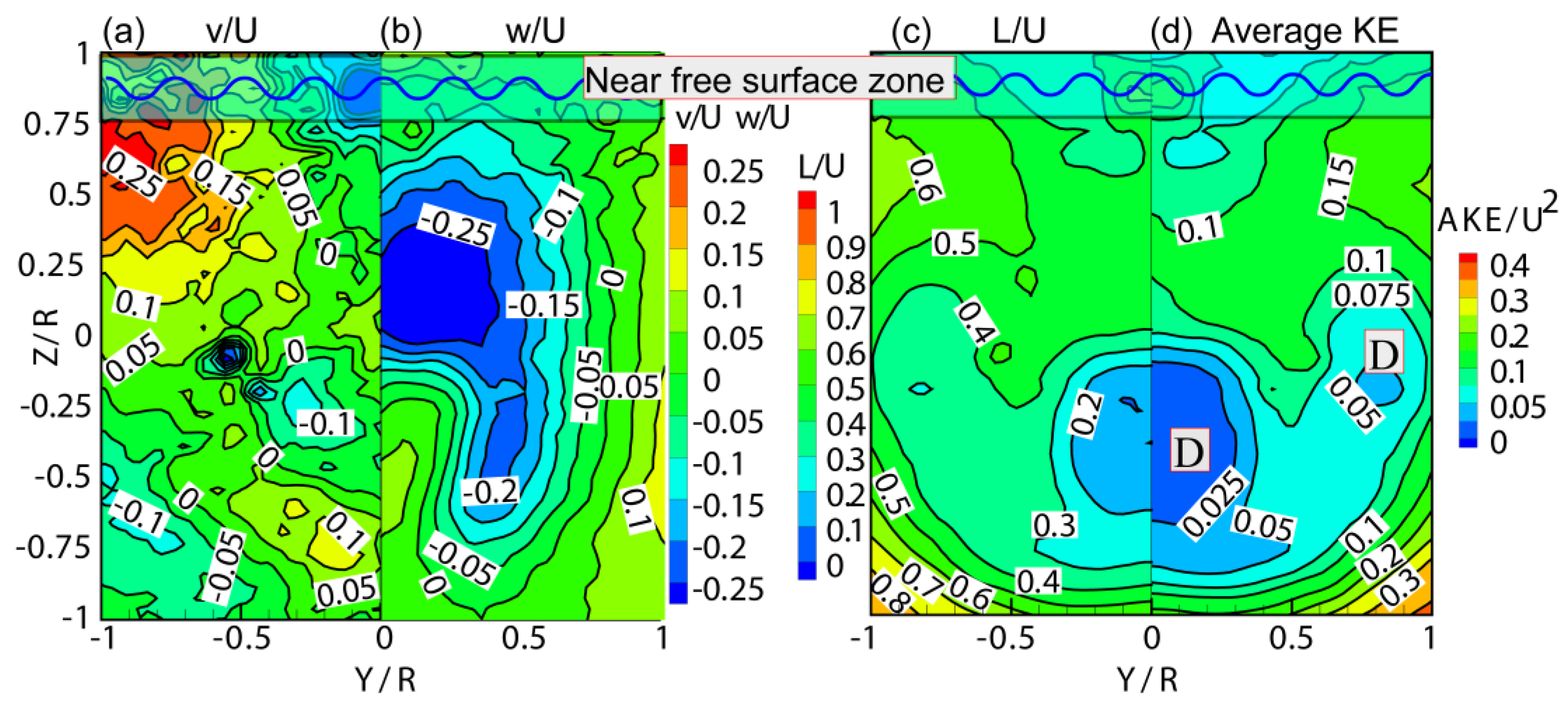The dimensionless axial flow velocity u/U, the cross-flow vector, cross-flow velocity S/U, and the streamline in the propeller region under the ballast and design conditions shown in Figure 3 and Figure 4a–d illustrates the results of the following parameters: the dimensionless transverse velocity v/U, vertical velocity w/U, whole-flow velocity L/U; and average kinetic energy AKE/U². The whole-flow velocity L ((u² + v² + w²)^1/2) and the cross-flow velocity S ((v² + w²)^1/2) conduct dimensionless processing with the towing speed of the ship model U. 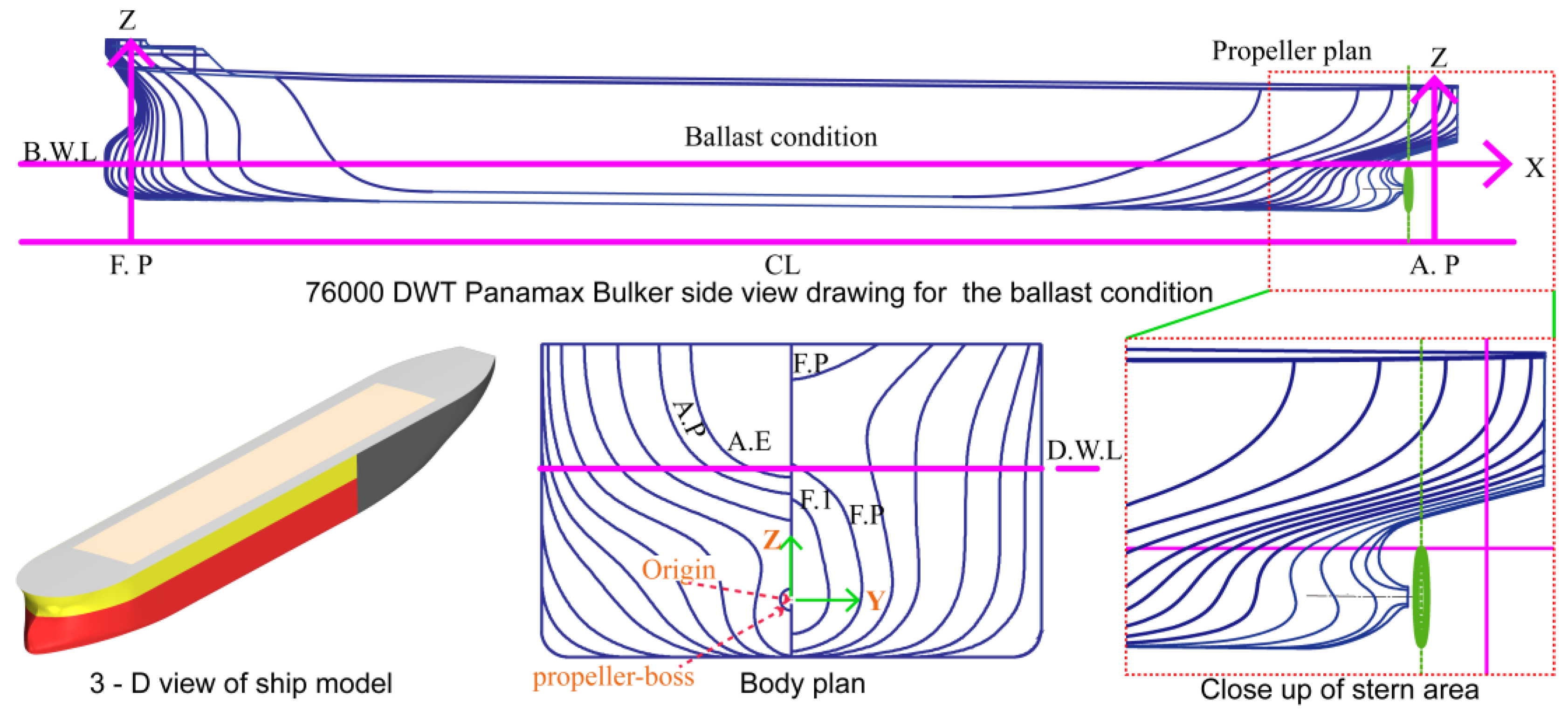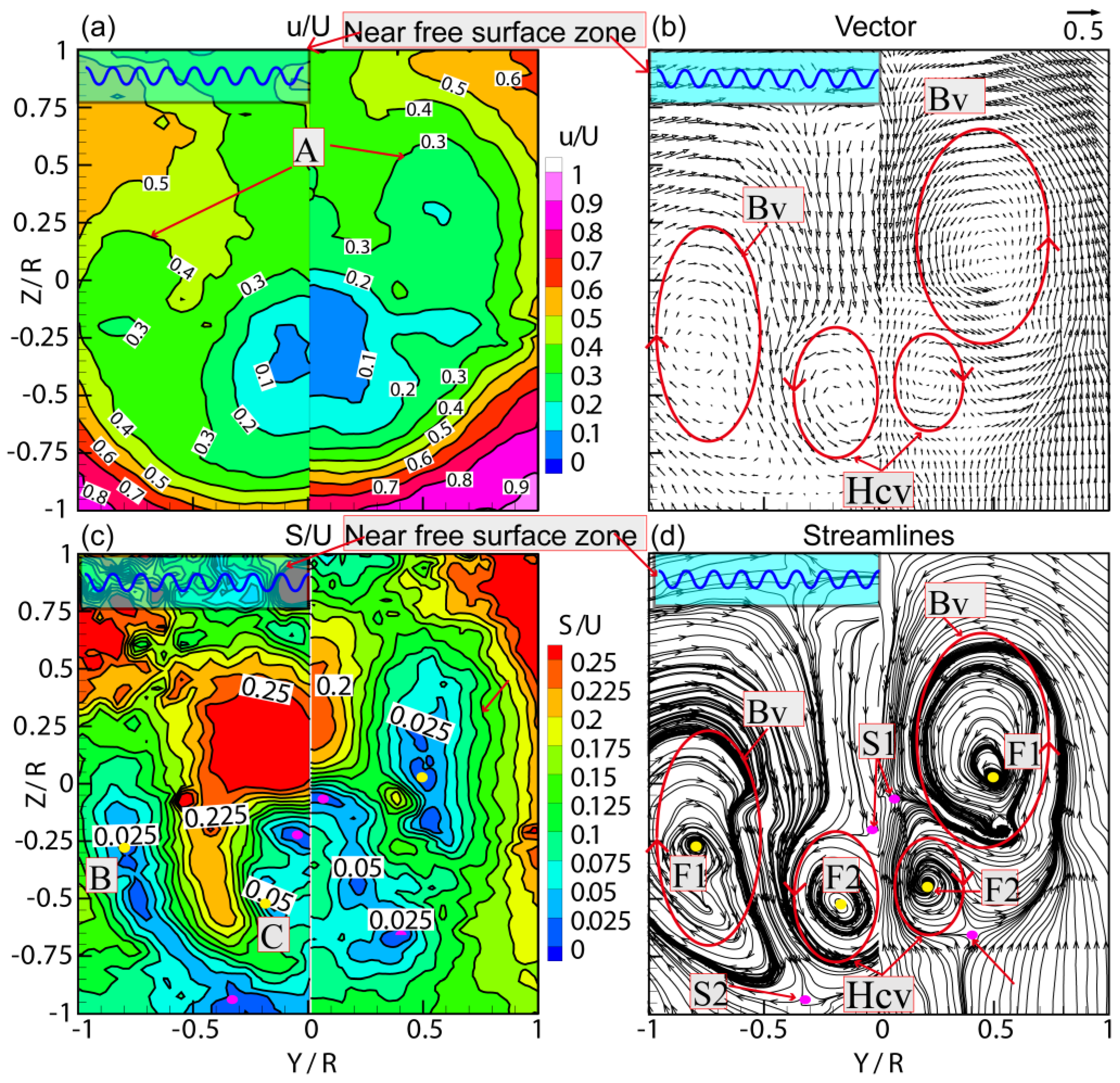The average kinetic energy (AKE = 1/2(u² + v² + w²)) conducts dimensionless processing with the square of the towing speed U². Under the ballast condition, the ship is a little trim by the stern and the draft is smaller than the design condition. Influenced by the change of the loading condition, the characteristics of the hook-like velocity contour can be found in Figure 3a, the distinct hook-like contours (labelled A) appear at the position of u/U = 0.4 (u/U = 0.3 under the design condition) [2], and the vertex of the hook-like contour is at the position of Z/R = 0.6 and Z/R = 0.25 under the design and ballast condition, respectively. The definition of hook-like characteristic, which was first proposed by Kim [6], is caused by flows with less average kinetic energy (Figure 4d, labeled D) being transferred through an intense longitudinal bilge vortex towards the center of the hull, which reduces its velocity and creates local hook-like structures. The bilge vortices formed by the flow passing through the stern of the U-shaped ship move down, which is almost in parallel with the hub cap vortices. The position of the hub cap vortex changes a little; however, the rotating range is larger than the design condition. The cross-flow vector and streamline clearly capture and illustrate the characteristics of the bilge vortex and the hub cap vortex. Figure 3c shows the contours of S/U. The bilge vortex foci (labelled F1) are at Y/R = ±0.5, Z/R = 0.05, and the hub cap vortex foci (labelled F2) are at Y/R = ±0.215, Z/R = −0.425 under the design condition. The bilge vortex foci (labelled F1) are at Y/R = ±0.75, Z/R = −0.25, and the hub cap vortex foci (labelled F2) are Y/R = ±0.215, Z/R = −0.55 under the ballast condition.

As the streamline shown in Figure 3d, on the starboard side of the ship, the bilge vortex flows counter-clockwise and the hub cap vortex flows clockwise. On the port side of the ship, the bilge vortex flows clockwise and the hub cap vortex flows counter-clockwise. The shape of the bilge vortex is "round" under the design condition. Under the ballast condition, the bilge vortex is in the shape of "ears", and the range of the hub cap vortex is larger than that under the design condition. In addition, the vortex foci of the twin vortex structure and the two saddle points of the propeller disk (labelled S1 and S2) are captured. The saddle point S1 is the intersection point of the upwash flow shear layer and the downwash flow shear layer. This is the point where the cross-section velocity S/U = 0 (S1 at Y/R = ±0.1, Z/R =−0.05, and Y/R = ±0.05, Z/R = −0.25 for the design and ballast condition, respectively). The saddle point S2 is the point where the left-wash flow and the right-wash flow separated from the up/down-wash flow shear layer and this is the point where the cross-section velocity S/U = 0 (S2 at Y/R = ±0.4, Z/R = −0.65, and Y/R = ±0.35, Z/R = −0.95 for the design and ballast condition, respectively).

It can be seen in Figure 4a,b that the positive and negative velocities represent the rotation direction of the bilge vortex and the hub cap vortex. This is because the ship is under the ballast condition and the top of the propeller disk area is near the free surface. The propeller disk area produces the near free surface layer disturbed by the free surface waveform. The dimensionless transverse velocity v/U and the dimensionless vertical velocity w/U are smaller than the dimensionless axial velocity u/U. These are greatly affected by the free surface disturbance. Therefore, the distribution of the dimensionless transverse velocity v/U and the dimensionless vertical velocity w/U in the near free surface layer is chaotic. Figure 4c,d shows that the hook-like region of the wake field in the propeller disk area has lower average kinetic energy (AKE) (labelled D in Figure 4d) characteristics due to the influence of the bilge vortex and the hub cap vortex.

3.2. Time-Averaged Velocity at Z/R = 0

Figure 5 shows the time-averaged velocity u/U, v/U, w/U, S/U, L/U, and AKE/U² profiles at Z/R = 0.00 in the propeller region under the ballast condition. The measurement results are as follows. The dimensionless axial velocity u/U and the whole-flow velocity L/U show an oscillatory profile from Y/R = 0 to Y/R = 1. The hook-like distributions of time-averaged velocity u/U and L/U first increase from Y/R = 0–0.5, then decrease from Y/R = 0.5–0.8, and finally increase from Y/R = 0.8–1.0. The velocity v/U increases first and then decreases at Y/R = 0.55. The velocity w/U shows a gradually decreasing trend from Y/R = 0 to Y/R = 1. Because of the larger range of the hook-like velocity profile under the ballast condition than that under the design condition, the distribution of S/U presents concave in the range Y/R = 0.5–1.0. It has a minimum velocity at Y/R = 0.85 with a magnitude of S/U = 0.065. The low kinetic energy AKE/U² appears in the range Y/R = 0–1.0 because of the disturbance caused by the hook-like velocity contours and the bilge vortex.

3.3. Time-Averaged Velocity at Each Radius

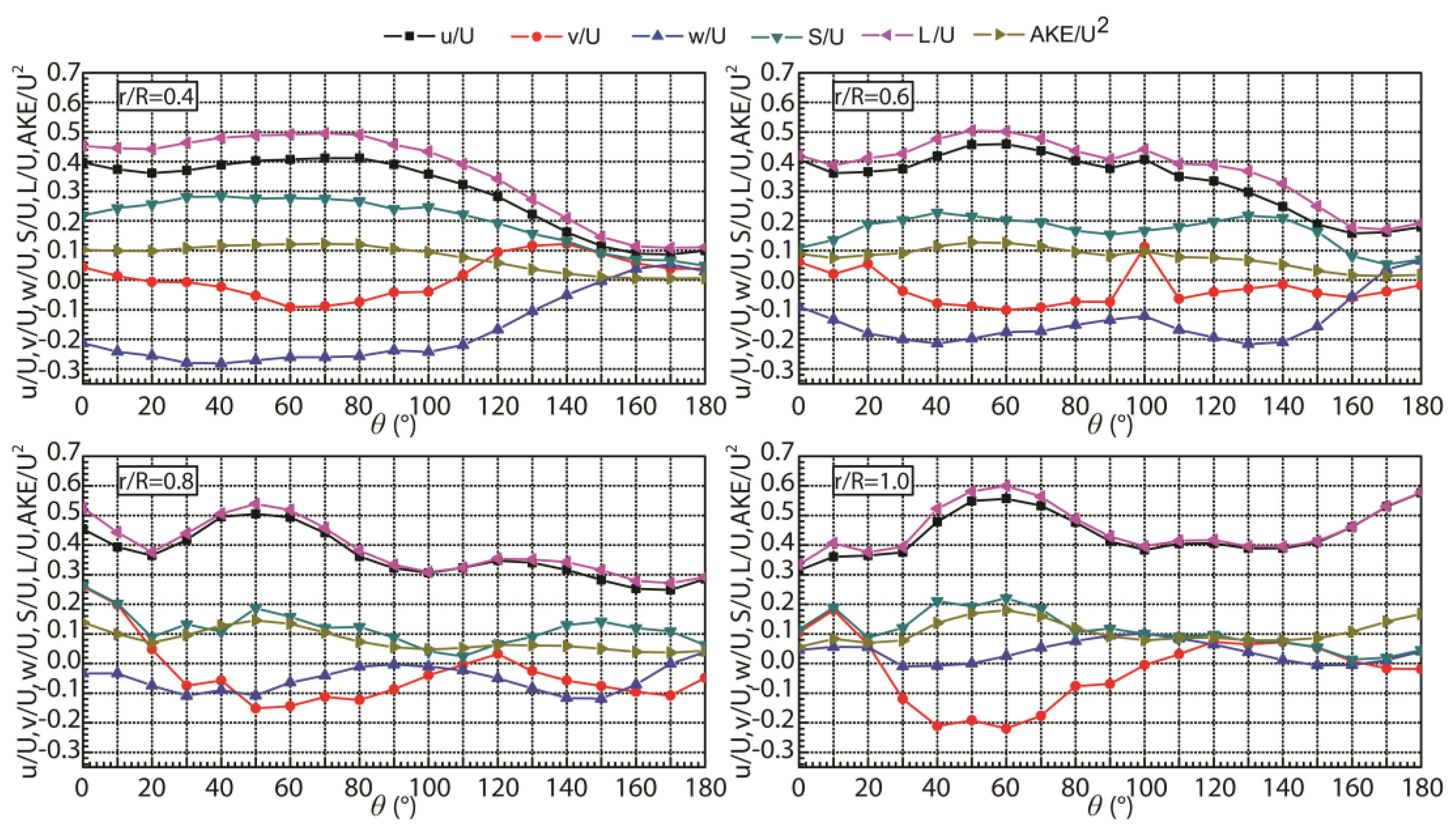
In this section, the velocity and the AKE/U² profiles with several radii (r/R = 0.4, 0.6, 0.8, 1.0) under the ballast condition are illustrated. Figure 6 shows the velocities u/U, v/U, w/U, S/U, L/U, and AKE/U². The circumferential angle θ runs clockwise from 0° (top) to 180°. When r/R = 0.4 and 0.6, as shown in Figure 6, the positive and negative values of the time-averaged velocity v/U and w/U represent the direction of these parameters. The time-averaged velocity u/U, S/U, L/U, and AKE/U² are basically positive and decrease with respect to θ, which is the same with that under the design condition. For r/R = 0.6, the cross-section velocity S/U has some slight fluctuations. The dimensionless transverse velocity v/U and w/U are basically negative. The "absolute" values of v/U and w/U with respect to the circumferential angle θ first increase and then decrease. At r/R = 0.8, the distributions of u/U, S/U, L/U, and AKE/U² with respect to θ show a decreasing trend followed by an increasing and decreasing trend. The "absolute" values of v/U and w/U with respect to the circumferential angle θ first increases and then it decreases with a relatively irregular change. However, the trend of S/U and AKE/U² are not significant and are relatively stable. When r/R = 1.0, u/U, S/U, L/U, and AKE/U² are increasing except for θ = 0–30° and 160–180° with a slight fluctuation (u/U, L/U). The dimensionless transverse velocity v/U exhibits strong fluctuations. The dimensionless vertical velocity w/U has a relatively stable distribution.

3.4. Velocity Fluctuations

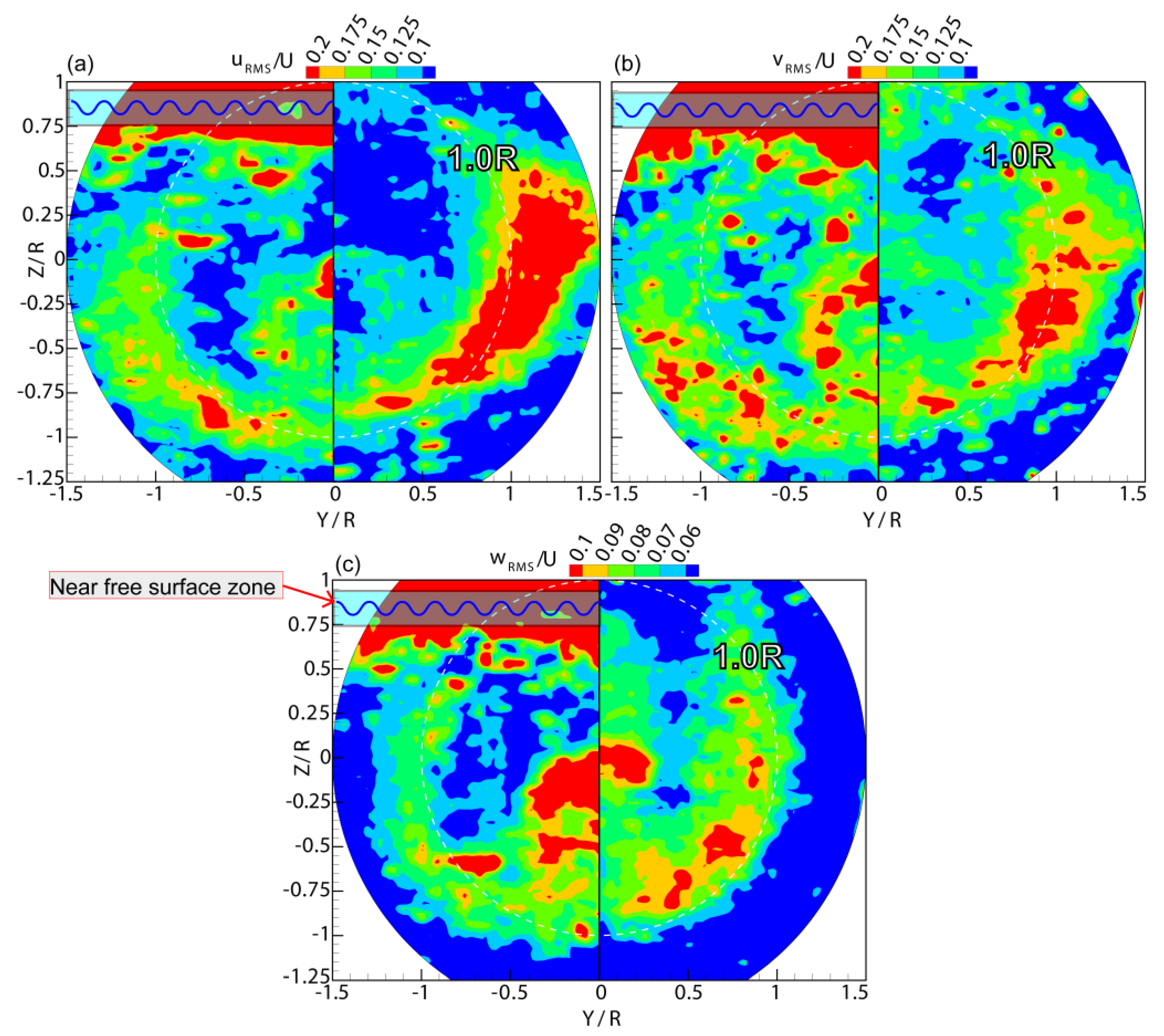
The turbulence characteristic of the flow fields is expressed as the root mean square velocity fields, which can be computed as: $u_{i-RMS}=u_i^{\prime }=\sqrt{\frac{1}{250}{\displaystyle \sum _{n=1}^{250}{(u_{i,n}-u_i)}^2}}$. Figure 7 shows the root mean square velocity fields under the ballast and design conditions. The root mean square velocity is dealt with a dimensionless method. Figure 7a–c displays the results of the dimensionless axial root mean square velocity u_RMS/U, the dimensionless transverse root mean square velocity v_RMS/U, and the dimensionless vertical root mean square velocity w_RMS/U, respectively. The white dotted line is the position where r/R = 1.0 and the light blue wavy line is near the free surface zone under the ballast condition. As depicted in Figure 7, the distribution of the root mean square velocity in the three directions is similar under the ballast and design conditions, which is either hook-shaped or U-shaped. Compared with that under the design condition, the areas with a strong fluctuation are mainly distributed at the end of the shaft, the range of r/R = 0.9–1.5, and the end of the hub cap. In addition, the top edge of the propeller is tangent to the free surface under the ballast condition, and a strong root mean square velocity fluctuation region is formed near the free surface.

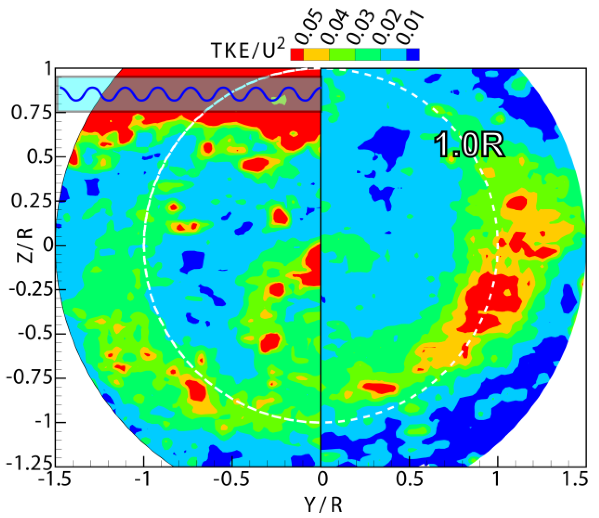
Figure 8 presents the TKE in the propeller region under the ballast and design conditions, Figure 9 presents the Reynolds stresses in the propeller region under the ballast condition. The Reynolds stresses tensor and TKE can be defined as: $\overline{u_i^{\prime }{u}_j^{\prime }}=\frac{1}{250}{\displaystyle \sum _{n=1}^{250}(u_{i,n}-u_i)(u_{j,n}-u_j)}$ and $TKE=1/2(\overline{u^{\prime }{u}^{\prime }}+\overline{v^{\prime }{v}^{\prime }}+\overline{w^{\prime }{w}^{\prime }})$, respectively, where i, j = 1, 2, 3 indicate the velocity fluctuations $u^{\prime }$, $v^{\prime }$, and $w^{\prime }$ in the x, y and z direction, respectively, u_i,n or u_{j, n} represents the n-th instantaneous velocity data. The TKE and the Reynolds stresses are dealt with the dimensionless method. 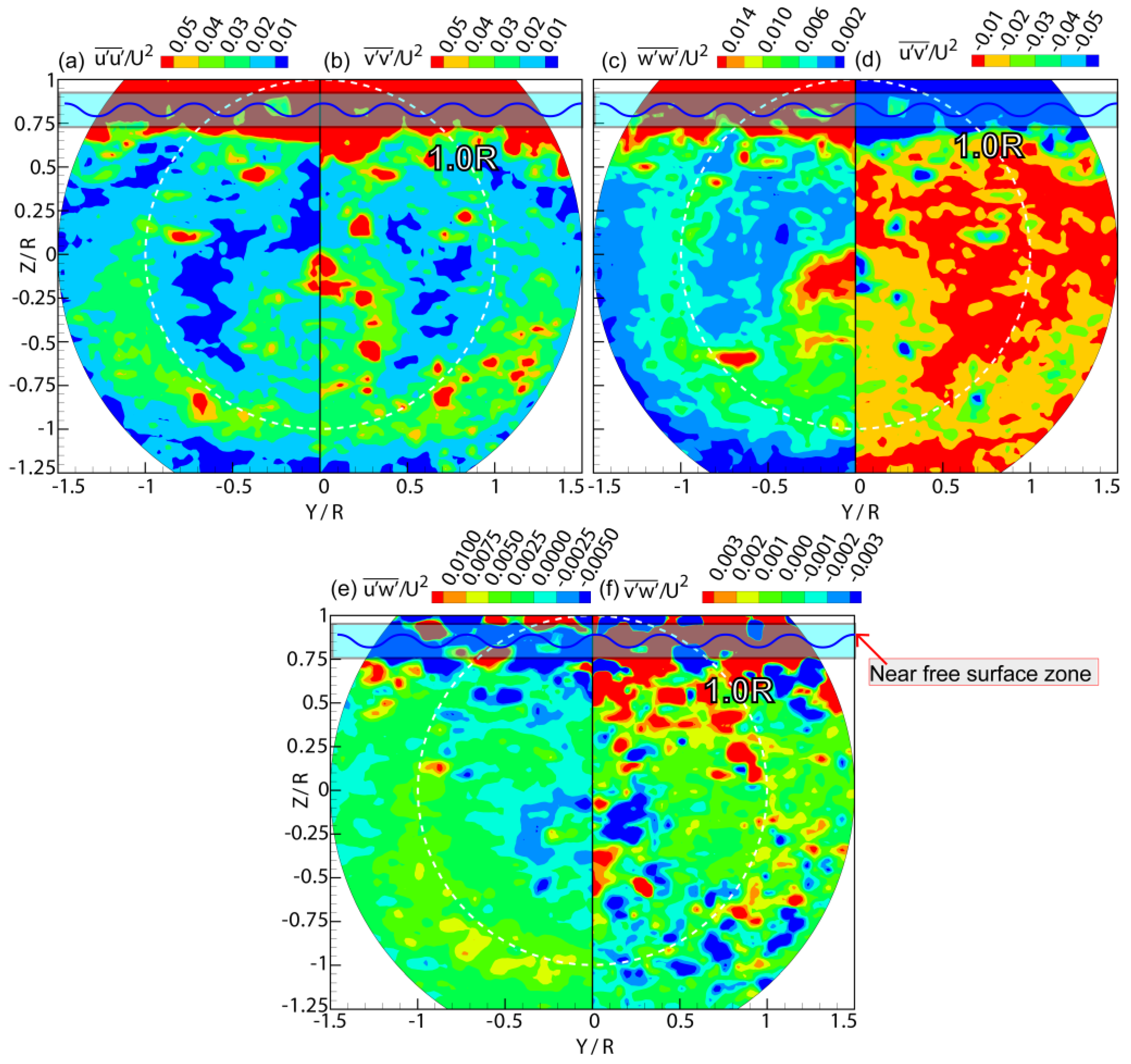Figure 9a–c displays the dimensionless Reynolds normal stress $\overline{u^{\prime }{u}^{\prime }}/U^2$, $\overline{v^{\prime }{v}^{\prime }}/U^2$, and $\overline{w^{\prime }{w}^{\prime }}/U^2$, respectively. Figure 9d–f depicts the dimensionless shear stress $\overline{u^{\prime }{v}^{\prime }}/U^2$, $\overline{u^{\prime }{w}^{\prime }}/U^2$, and $\overline{v^{\prime }{w}^{\prime }}/U^2$, respectively, and the white dotted line shows the position of r/R = 1.0.

As demonstrated in Figure 8, the distribution of the TKE is also U-shaped; however, the interval is wider and the U-shaped distribution is concentrated in the kinetic energy change layer, which is the transition from low kinetic energy to high kinetic energy. Compared with that under the design condition, the changing layer with strong gradient of the turbulent kinetic energy under the ballast condition is outward-transferring to 0.9R. Due to the influence of the loading condition, the shaft is no longer in the hydrodynamic downstream state under the ballast condition. Therefore, the TKE at the end of the shaft in the non-downstream state has a large amplitude. As demonstrated in Figure 9, the axial Reynolds normal stress $\overline{u^{\prime }{u}^{\prime }}/U^2$, the transverse Reynolds normal stress $\overline{v^{\prime }{v}^{\prime }}/U^2$, and the vertical Reynolds normal stress $\overline{w^{\prime }{w}^{\prime }}/U^2$ have the characteristic of anisotropy. The influence of the shallow draft at the stern under the ballast condition makes the propeller disk area have a turbulent area of about 0.25R near the free surface. Due to the influence of the rooster tail near the free surface, the TKE and the Reynolds stress in the turbulent region have a large amplitude. The maximum value of the axial Reynolds normal stress $\sqrt{\overline{u^{\prime }{u}^{\prime }}}$ ≈ 0.07U, the transverse Reynolds normal stress $\sqrt{\overline{v^{\prime }{v}^{\prime }}}$ ≈ 0.05U, and the vertical Reynolds normal stress $\sqrt{\overline{w^{\prime }{w}^{\prime }}}$ ≈ 0.016U in the non-interference region. The contours of the TKE are similar with the axial Reynolds normal stress $\overline{u^{\prime }{u}^{\prime }}/U^2$. The maximum TKE occurs in the high shear zone and the velocity gradient of the axial velocity component is large. This is because the axial Reynolds normal stress is much larger than the maximum of the transverse and vertical Reynolds normal stress.

The distribution of the Reynolds shear stress $\overline{u^{\prime }{v}^{\prime }}/U^2$, $\overline{u^{\prime }{w}^{\prime }}/U^2$, and $\overline{v^{\prime }{w}^{\prime }}/U^2$ is similar to the Reynolds normal stress and the TKE, which is U-shaped, except that the U-shape distribution of $\overline{v^{\prime }{w}^{\prime }}/U^2$ is not obvious. The propeller disk is also affected by the U-shaped stern and it has a U-shaped shear layer. However, due to the influence of the draft under the ballast condition, the underwater shape of the U-shaped stern is different from that under the design condition; thus, resulting in a different U-shaped shear layer. The shear layer under the ballast condition covers the bilge vortex and hub cap vortex in a wider range. The Reynolds shear stress $\overline{u^{\prime }{v}^{\prime }}/U^2$ is negative, where ∂u/∂Y is decreasing and it has a maximum value of $\sqrt{\overline{u^{\prime }{v}^{\prime }}}$ ≈ −0.05U. The Reynolds shear stress $\overline{u^{\prime }{w}^{\prime }}/U^2$ has similar behavior; however, it is correlated with ∂u/∂Z and it attains a maximum of $\sqrt{\overline{u^{\prime }{w}^{\prime }}}$ ≈ 0.01U. The vertical Reynolds shear stress $\overline{v^{\prime }{w}^{\prime }}/U^2$ represents the turbulent shear characteristics of the y-z section of the propeller disk. Compared with that under the design condition, the U-shaped shear layer in the outer region of the two vortices is slightly weaker than that under the design condition. In addition, the turbulent region near the free surface also has a great influence on the Reynolds shear stress in the range of Z/R = 0.75–1.0R.

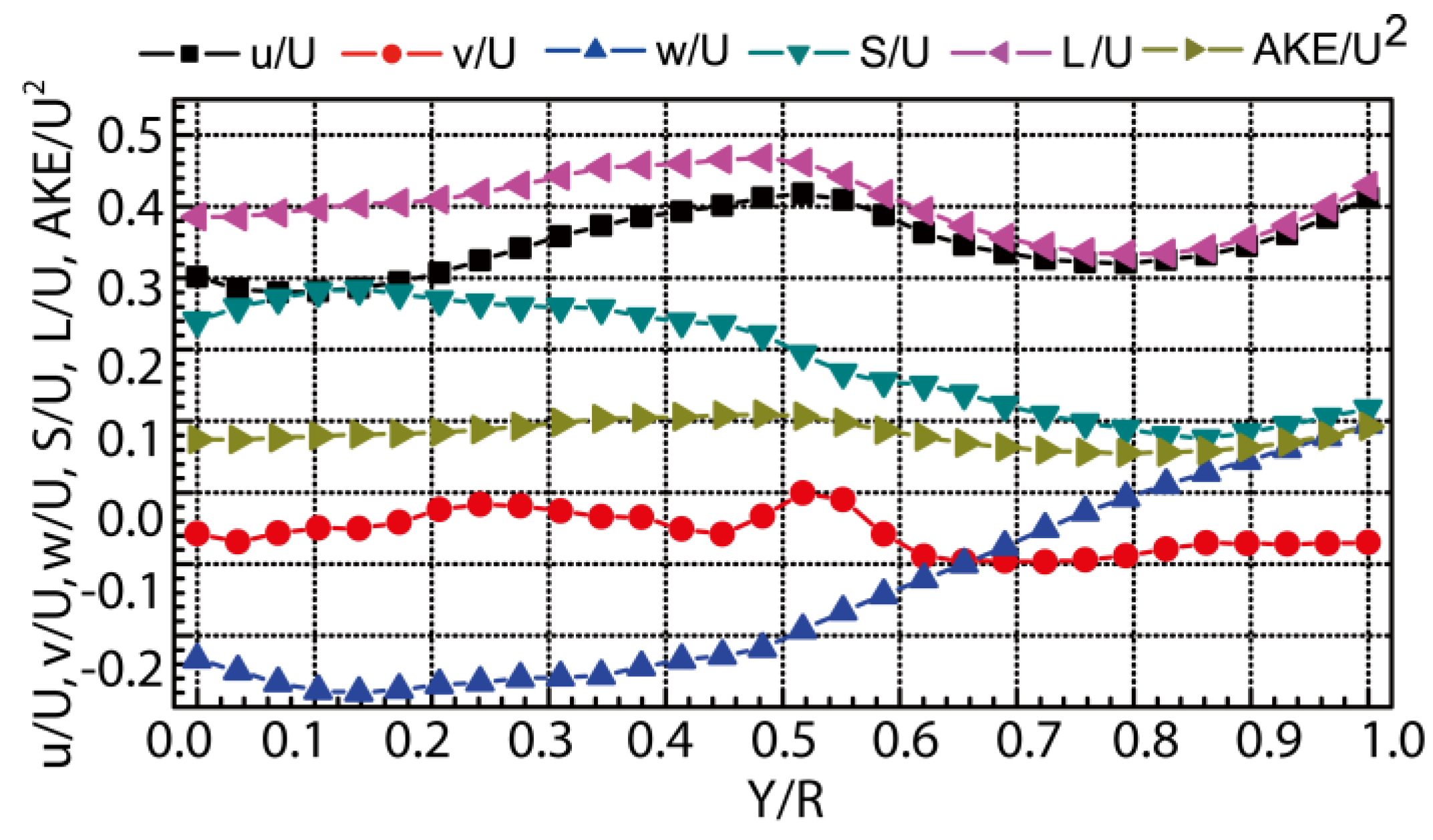
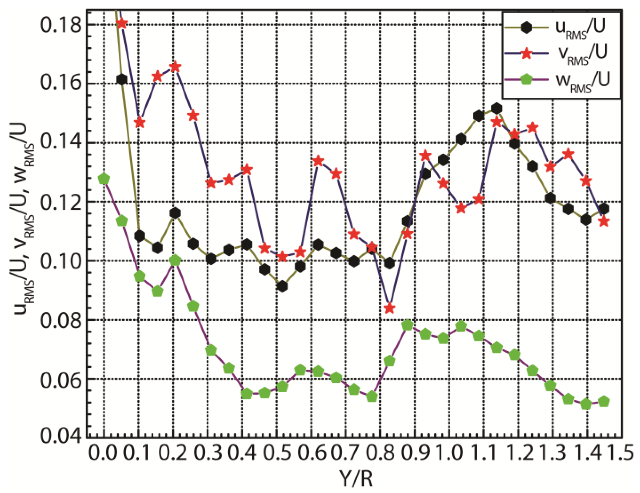
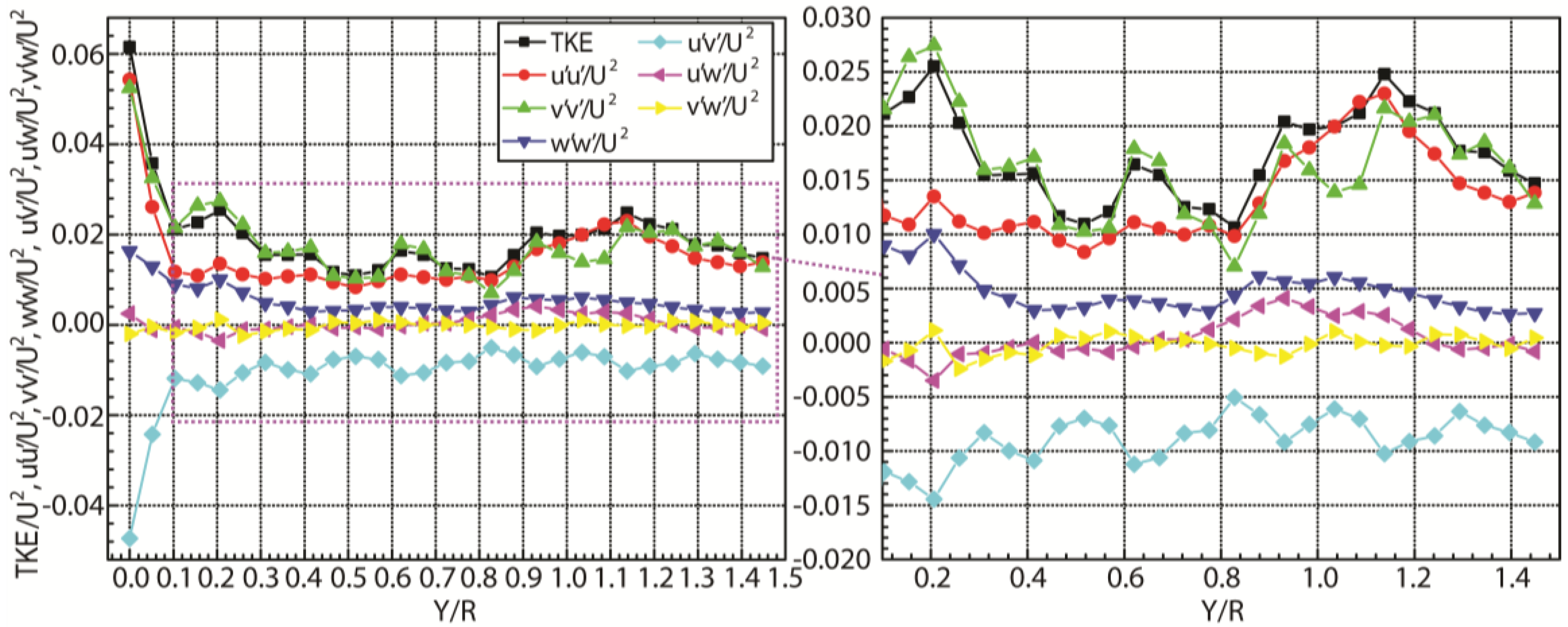
Figure 10 depicts the root mean square velocity profiles at Z/R = 0.00 under the ballast condition, which is a quantitative expression of the distribution of the turbulent fluctuating velocity field. The results show that the dimensionless turbulent fluctuating velocity first decreases, then it increases, and it finally decreases from Y/R = 0 to Y/R = 1. Figure 11 displays the turbulence statistics at Z/R = 0.00 under the ballast condition. The dimensionless Reynolds normal stress $\overline{u^{\prime }{u}^{\prime }}/U^2$, $\overline{v^{\prime }{v}^{\prime }}/U^2$, $\overline{w^{\prime }{w}^{\prime }}/U^2$, and TKE/U² show an overall decreasing distribution from Y/R = 0 to Y/R = 1. The dimensionless Reynolds shear stress $\overline{u^{\prime }{v}^{\prime }}/U^2$ is increasing. The dimensionless Reynolds shear stress $\overline{u^{\prime }{w}^{\prime }}/U^2$ and $\overline{v^{\prime }{w}^{\prime }}/U^2$ show a relatively flat trend of change. As illustrated in Figure 11 on the right for the close up of the turbulence statistics profiles, the dimensionless Reynolds normal stress $\overline{u^{\prime }{u}^{\prime }}/U^2$, $\overline{v^{\prime }{v}^{\prime }}/U^2$, TKE/U², and the Reynolds shear stress $\overline{u^{\prime }{v}^{\prime }}/U^2$ have been acutely fluctuating.

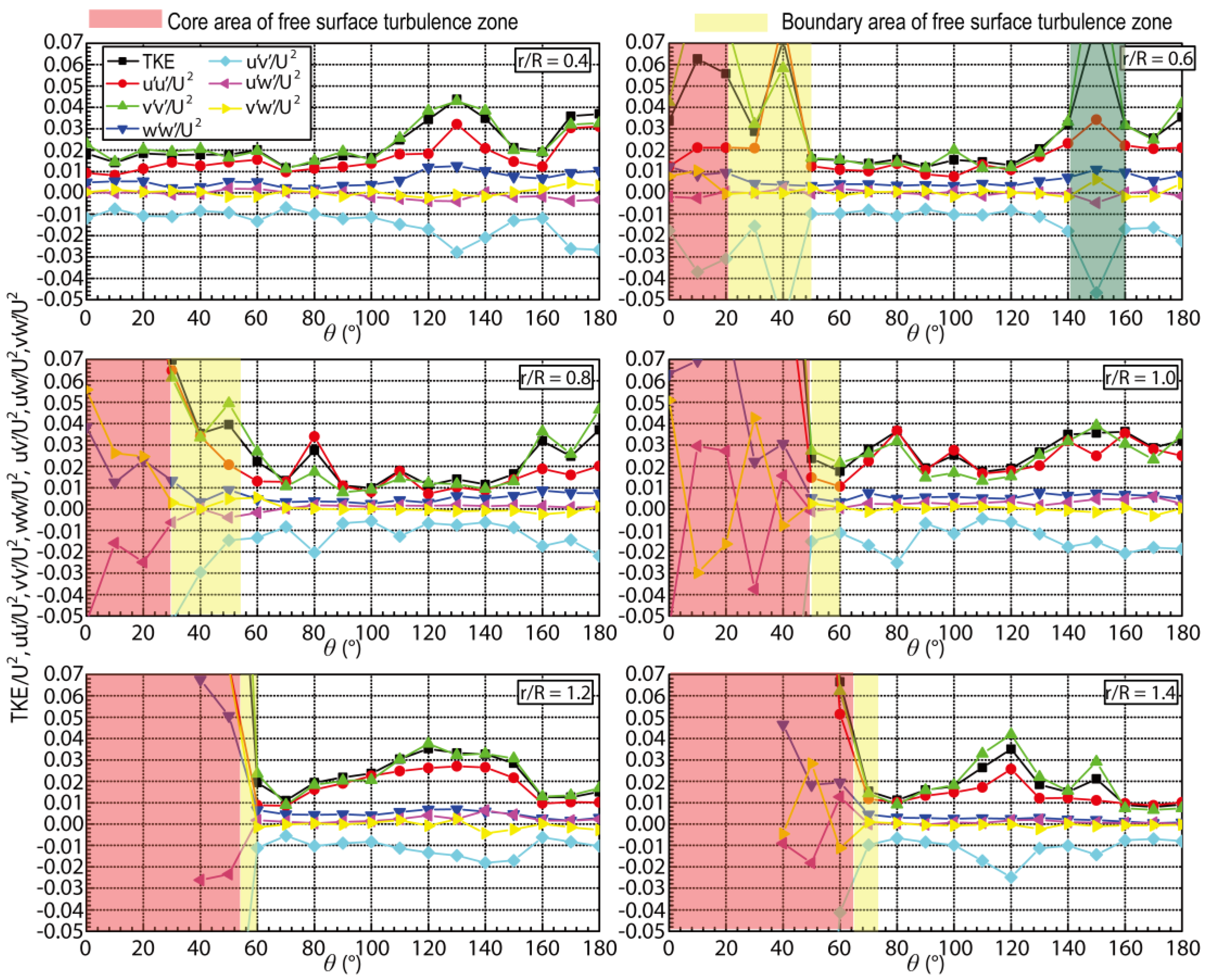
Figure 12 presents the turbulence statistics profiles at different radius in the propeller region under the ballast condition and the interval is 10°. Among them, the 0° circumferential angle is directly above the propeller disk surface and the circumferential angle gradually increases clockwise to 180°. The red area is near the free surface wave core turbulent area, the yellow area is the boundary area affected by the core area, and the green frame is the local high-turbulence area in the propeller disk.

In the circumferential distribution area with a radius r/R = 0.4, the TKE and Reynolds stress at the end of the shaft show a relatively stable distribution trend with increasing circumferential angle, and the peak distribution appears in the corresponding area at the end of the shaft. In the region with r/R = 0.6–0.8, which is located in the low-kinetic-energy region, the TKE and Reynolds stress are relatively stable as the circumferential angle increases. In the circumferential distribution area with r/R = 1.0–1.4, the curves of the points taken from the circumferential distribution are in the average kinetic energy change layer region. With the increase in the circumferential angle, the dimensionless TKE and the Reynolds normal stress present a relatively violent fluctuation distribution as a whole. In addition, the near free surface wave core turbulent region in red and the boundary region affected by the yellow core have a large amplitude and a violent fluctuation. The shape of the stern has typical longitudinal curvature and cross-sectional curvature (see Figure 1). The anisotropic turbulent flow of the wake has a strong correlation with the longitudinal curvature and cross-sectional curvature of the stern as well as the flow gathering and dispersion around the stern. The local geometry in the stern region of the ship is different at different span wise and circumferential angle positions, and thus the average velocity and turbulence characteristic are different at various span wise and circumferential angle positions. Figure 6, Figure 10, Figure 11 and Figure 12 in the article illustrate the average velocity and turbulence characteristic parameters at different span and circumferential angle positions. The trend is closely related to the flow nature, and it should be pointed out that it also includes measurement uncertainty factors. But the main factor is the flow factor, and uncertainty has little effect on the overall distribution characteristics and distribution trends.

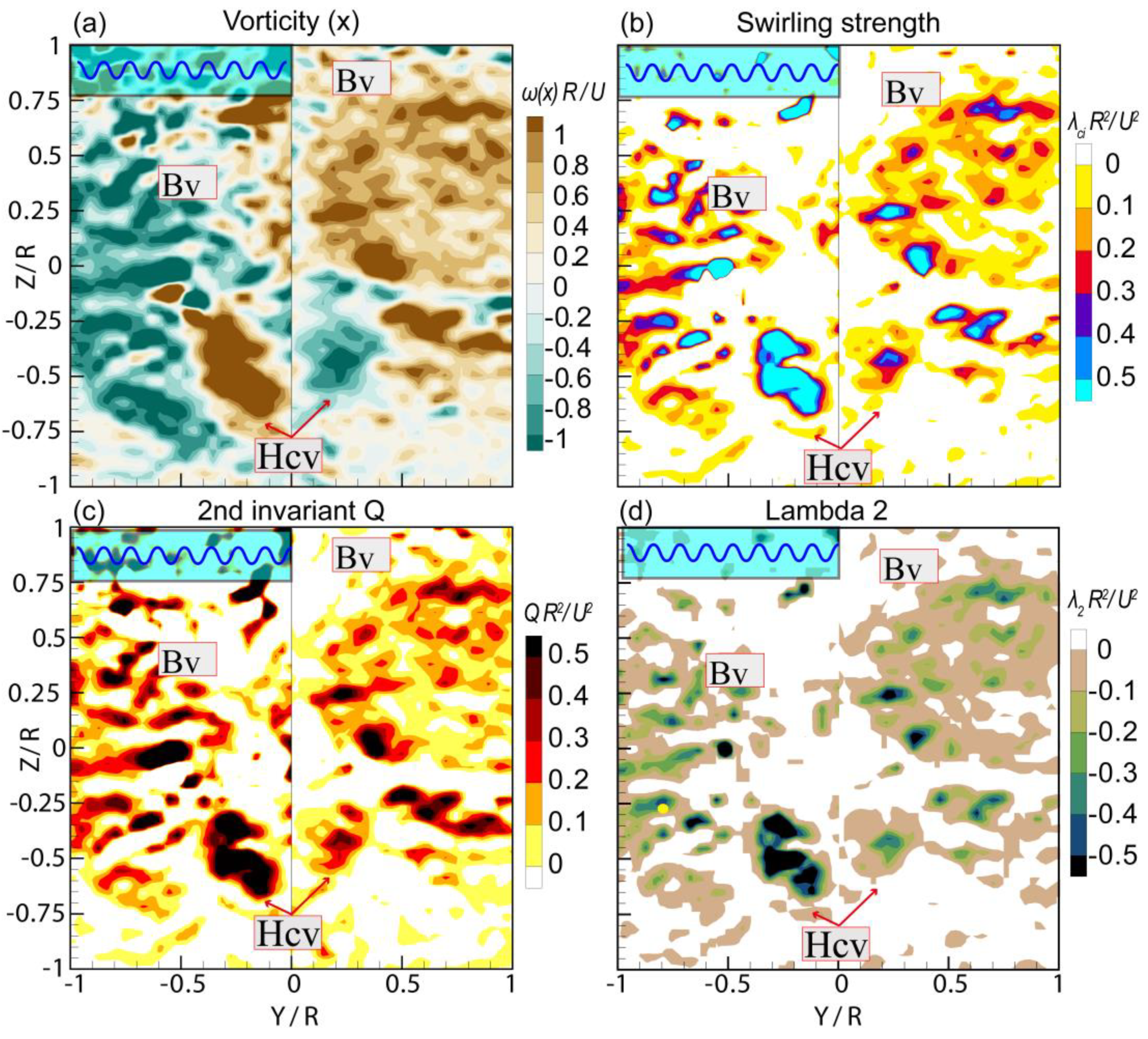
3.5. Vorticity Information

Figure 13 shows the vorticity information under the ballast and design conditions. Figure 13a shows the contour maps of the vorticity (x) which can be computed as: $Vorticity(x)={\omega }_x=\frac{\partial w}{\partial y}-\frac{\partial v}{\partial z}$, and the positive value of the vorticity (x) indicates that the rotation direction of the vortex is counter clockwise and the negative value is clockwise. Figure 13b shows the contour maps of the swirling strength, and the swirl strength is defined as the imaginary part of the complex eigen-value of the velocity gradient tensor [21,22], and the square of the imaginary part can be computed as:${\lambda }_{ci}=\frac{1}{2}\sqrt{-4\left(\frac{\partial W}{\partial y}\frac{\partial V}{\partial z}-\frac{\partial V}{\partial y}\frac{\partial W}{\partial z}\right)-{\left(\frac{\partial V}{\partial y}+\frac{\partial W}{\partial z}\right)}^2}$, Figure 13c shows the contour maps of the planar 2nd invariant Q, the 2nd invariant Q of the velocity gradient matrix [23,24], which can be used to identify vortices, can be defined as $Q=-\left(\frac{\partial W}{\partial y}\frac{\partial V}{\partial z}-\frac{\partial V}{\partial y}\frac{\partial W}{\partial z}\right)-\frac{1}{2}{\left(\frac{\partial V}{\partial y}+\frac{\partial W}{\partial z}\right)}^2$. Figure 13d shows the contour maps of the lambda 2 criterion, detailed definitions and calculation formulas of the lambda 2 criterion can be found in the literature [24], The vorticity (x), swirling strength, 2nd invariant Q and lambda 2 conducts dimensionless processing by multiply R/U and R²/U², respectively, where R is the propeller and U is the towing speed. The local minimum negative value of lambda-2 can be used to identify the vortex core, while the positive value indicates the flow field, and the shear flow may be displayed but not rotated. The local maximum positive value of the swirling strength and planar 2nd invariant Q can be used to identify the vortex core. A strong bilge vortex (Bv) will be produced when the water flows through the U-shaped stern. There is a propeller hub cap vortex (Hcv) under the bilge vortex, which is opposite to the rotation direction of the bilge vortex, and the hub cap vortex is close to the longitudinal section of the ship. Under the ballast condition, the ship has a trim by the stern, and the draft is smaller than that under the design condition. Influenced by the position of the ship, the bilge vortex formed by the U-shaped stern moves down, which is almost in parallel with the hub cap vortex. The position of the hub cap vortex changes a little bit; however, the rotating range is larger than that under the design condition. The lambda 2-criterion, the vorticity, and planar 2nd invariant Q all recognize the bilge vortices and the propeller hub cap vortex. The positive value of the vorticity (x) indicates that the local vortex rotates anticlockwise and vice versa. The bilge vortex generated by the bilge area in the middle of the hull rotates anticlockwise on the port side and on the starboard side. In addition, it is transmitted to the propeller disk, and it is located within the velocity contour range from u/U = 0.3 to u/U = 0.5 (Figure 3). The hub cap vortex has the opposite rotation direction to the bilge vortex and it is generated by the hub at the installation position of the propeller on the shaft of the hull. In addition, it is transmitted to the propeller disk area along with the wake. The hub cap vortex is located along the velocity contour range of u/U < 0.3 (Figure 3). According to the contour of the vorticity and swirling strength, the bilge vortex on the propeller disk appears “round-like” under the design condition and is “ear-like” under the ballast condition.

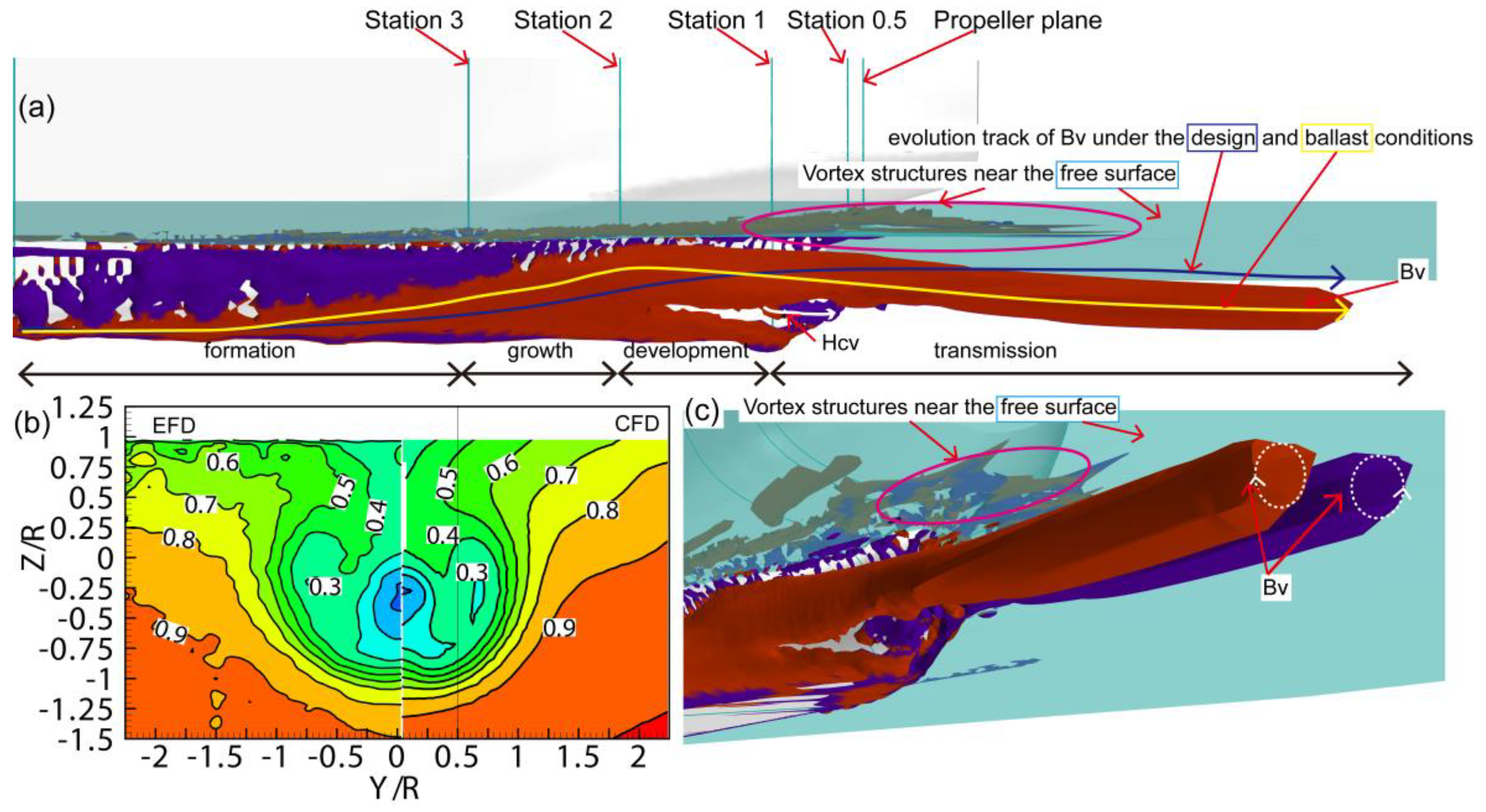
In order to analyze the vortex evolution characteristics of Panama bulk carriers under ballast condition, CFD numerical simulation analysis was carried out using the formed calculation strategy [2,25]. Figure 14 is the vortex evolution of Panama bulk carrier under the ballast condition based on CFD. As shown in Figure 14b, the CFD numerical results agree well with the PIV measurement results, which verifies the accuracy of the numerical calculation. Figure 14a,c is the global evolution and close-up view of the vortex structure, under the ballast condition. In addition to the bilge vortex and hubcap vortex similar to the design one, there are also vortex structures near the free surface caused by fluctuations of free surface. In addition, the evolution trajectories of the bilge vortex and the hub cap vortex in ballast are different from the design ones.

4. Conclusions

The wake fields of the test model under the ballast condition is experimentally investigated based on the authors’ previous research, which is under the design condition. The wake field data includes time-averaged, turbulence characteristics, and vorticity information. When comparing the results under the design condition, it can be concluded as follows.

(1) The time-averaged velocity contours indicate that the ballast and design conditions have distinct hook-like axial velocity contours, but they appear at different positions. The distinct hook-like axial velocity contours appear at the position of u/U = 0.3 and the vertex of the hook-like contour is at the position of Z/R = 0.6 under the design condition. Under the ballast condition, the distinct hook-like axial velocity contours appear at the position of u/U = 0.4 and the vertex of the hook-like contour is at the position of Z/R = 0.25. The shape of the bilge vortex is "round-like" under the design condition, but it has an “ear-like” shape under the ballast condition. The big difference under the ballast condition is that the top of the propeller disk area is near the free surface. The propeller disk area produces the near free surface layer that is disturbed by the free surface waveform. The vortex foci of the twin vortex structure and the two saddle points (S1 and S2) of the propeller disk are captured under the ballast and design conditions. Under the design condition, the saddle point S1 at Y/R = ±0.1, Z/R = −0.05, S2 at Y/R = ±0.4, and Z/R = −0.65. Under the ballast condition, the saddle point S1 at Y/R = ±0.025, Z/R = −0.25, S2 at Y/R= ±0.35, and /R= −0.9.

(2) In comparison to the design condition, the areas with strong fluctuation are mainly distributed at the end of the shaft, the range of r/R = 0.9–1.5, and the end of the hub cap. In addition, the top edge of the propeller is tangent to the free surface under the ballast condition, and a strong root mean square velocity fluctuation region is formed near the free surface. The TKE, Reynolds stresses, and the hub cap vortex are all affected by the turbulent velocity fluctuation region under the ballast condition. The interval is wider and the U-shaped distribution is concentrated in the kinetic energy change layer under the ballast condition. The shear layer under the ballast condition covers the bilge vortex and the hub cap vortex in a wider range.

(3) A strong bilge vortex (Bv) is produced when the water flows through the U-shaped stern under the design and ballast conditions. Under the ballast condition, the bilge vortex formed by the U-shaped stern moves down, which is almost in parallel with the hub cap vortex. The position of the hub cap vortex changes a little bit; however, the rotating range is larger than that under the design condition. According to the contour of the vorticity and the swirling strength, the bilge vortex on the propeller disk appears "round" under the design condition and it resembles an "ear" under the ballast condition.

References

1. Asariotis, R.; Assaf, M.; Benamara, H.; Hoffmann, J.; Premti, A.; Rodríguez, L.; Weller, M.; Youssef, F. Review of Maritime Transport, United Nations. 2018. Available online: https://shop.un.org/series/review-maritime-transport (accessed on 26 May 2020).
2. Guo, C.Y.; Wu, T.C.; Luo, W.Z.; Chang, X.; Gong, J.; She, W.X. Experimental study on the wake fields of a Panamax Bulker based on stereo particle image velocimetry. Ocean. Eng. 2018, 165, 91–106. [Google Scholar] [CrossRef]
3. Lee, J.Y.; Paik, B.G.; Lee, S.J. PIV measurements of hull wake behind a container ship model with varying loading condition. Ocean. Eng. 2009, 36, 377–385. [Google Scholar] [CrossRef]
4. Park, D.; Kim, Y.; Seo, M.; Lee, J. Study on added resistance of a tanker in head waves at different drafts. Ocean. Eng. 2016, 111, 569–581. [Google Scholar] [CrossRef] [Green Version]
5. Dong, R.R.; Katz, J.; Huang, T.T. On the structure of bow waves on a ship model. J. Fluid Mech. 1997, 346, 77–115. [Google Scholar] [CrossRef]
6. Kim, W.J.; Van, S.H.; Kim, D.H. Measurement of flows around modern commercial ship models. Eperiments Fluids 2001, 31, 567–578. [Google Scholar] [CrossRef]
7. Lee, S.J.; Koh, M.S.; Lee, C.M. PIV velocity field measurements of flow around a KRISO 3600TEU container ship model. J. Mar. Sci. Technol. 2003, 8, 76–87. [Google Scholar] [CrossRef]
8. Lee, S.J.; Kim, H.R.; Kim, W.J.; Van, S.H. Wind tunnel tests on flow characteristics of the KRISO 3600 TEU containership and 300K VLCC double-deck ship models. J. Ship Res. 2003, 47, 24–38. [Google Scholar]
9. Calcagno, G.; Di Felice, F.; Felli, M.; Pereira, F. A stereo-PIV investigation of a propeller’s wake behind a ship model in a large free-surface tunnel. Mar. Technol. Soc. J. 2005, 39, 94–102. [Google Scholar] [CrossRef]
10. Falchi, M.; Felli, M.; Grizzi, S.; Aloisio, G.; Broglia, R.; Stern, F. SPIV measurements around the DELFT 372 catamaran in steady drift. Exp. Fluids 2014, 55, 1844. [Google Scholar] [CrossRef]
11. Yoon, H.; Longo, J.; Toda, Y. Benchmark CFD validation data for surface combatant 5415 in PMM maneuvers–Part II: Phase-averaged stereoscopic PIV flow field measurements. Ocean. Eng. 2015, 109, 735–750. [Google Scholar] [CrossRef] [Green Version]
12. Gui, L.; Longo, J.; Stern, F. Towing tank PIV measurement system, data and uncertainty assessment for DTMB model 5512. Exp. Fluids 2001, 31, 336–346. [Google Scholar] [CrossRef]
13. Seo, J.; Seol, D.M.; Han, B.; Rhee, S.H. Turbulent wake field reconstruction of VLCC models using two-dimensional towed underwater PIV measurements. Ocean. Eng. 2016, 118, 28–40. [Google Scholar] [CrossRef] [Green Version]
14. Wu, P.C. A CFD Study on Added Resistance, Motions and Phase Averaged Wake Fields of Full form Ship Model in Head Waves. Ph.D. Thesis, Osaka University, Osaka, Japan, July 2013. [Google Scholar]
15. Wu, P.C.; Okawa, H.; Kim, H.; Akamatsu, K.; Sadat-Hosseini, H.; Stern, F.; Toda, Y. Added resistance and nominal wake in waves of KVLCC2 model ship in ballast condition. In Proceedings of the 30th Symposium on Naval Hydrodynamics, Hobart, Tasmania, Australia, 2–7 November 2014; pp. 2–7. [Google Scholar]
16. Luo, W.Z.; Guo, C.Y.; Wu, T.C.; Dai, S.S.; Su, Y.M. Numerical simulation of viscous flow field around ships in ballast. J. Coastal Res. 2016, 32, 911–922. [Google Scholar] [CrossRef]
17. Guo, C.Y.; Wu, T.C.; Zhang, Q.; Gong, J. Numerical simulation and experimental research on wake field of ships under off-design conditions. China Ocean. Eng. 2016, 30, 821–834. [Google Scholar] [CrossRef]
18. The Propulsion Committee. In Proceedings of the 25th ITTC, Fukuoka, Japan, 14–20 September 2008; Volume II.
19. Bendat, J.S.; Piersol, A.G. Random Data—Analysis and Measurement Procedures; John Wiley & Sons, Inc.: Hoboken, NJ, USA, 1986. [Google Scholar]
20. Bendat, J.S.; Piersol, A.G. Random Data; John Wiley & Sons, Inc.: Hoboken, NJ, USA, 2010. [Google Scholar]
21. Adrian, R.J.; Christensen, K.T.; Liu, Z.C. Analysis and interpretation of instantaneous turbulent velocity fields. Exp. Fluids 2000, 29, 275–290. [Google Scholar] [CrossRef]
22. Hunt, J.C.; Wray, A.A.; Moin, P. Eddies, Streams, and Convergence Zones in Turbulent Flows. Center for Turbulence Research Report CTR-S88. 1988, p. 193. Available online: https://ui.adsabs.harvard.edu/abs/1988stun.proc..193H/abstract (accessed on 30 May 2020).
23. Chong, M.S.; Perry, A.E.; Cantwell, B.J. A general classification of three-dimensional flow fields. Phys. Fluids Fluid Dyn. 1990, 2, 765–777. [Google Scholar] [CrossRef]
24. Jeong, J.; Hussain, F. On the identification of a vortex. J. Fluid Mech. 1995, 285, 69–94. [Google Scholar] [CrossRef]
25. Wu, T.C.; Guo, C.Y.; Luo, W.Z. Experimental and Numerical Study on the Wake Field of a 76000 DWT Panamax Bulker. In Proceedings of the 8th International Conference on Computational Methods (ICCM2017), Guilin, China, 25–29 July 2017; pp. 813–820. [Google Scholar]
Figure 1. Lines plan and the geometric model.
Jmse 08 00397 g001
Figure 2. Experimental setup of SPIV measurement: (a) photograph of SPIV setup in the towing tank; (b) schematic diagram of SPIV setup; (c) close-up of the position of the propeller plane and PIV system; (d) close-up of the position of the propeller plane, free surface, and laser sheet.
Jmse 08 00397 g002
Figure 3. The time-averaged characteristics of the velocity information in the propeller plane: (a) dimensionless axial flow velocity u/U; (b) the cross-flow vector; (c) dimensionless cross-flow velocity S/U; (d) streamline. For (ad), Left. The ballast condition; Right. The design condition.
Jmse 08 00397 g003
Figure 4. The time-averaged characteristics of the velocity information in the propeller plane under ballast condition: (a) dimensionless transverse velocity v/U; (b) dimensionless vertical velocity w/U; (c) dimensionless whole-flow velocity L/U; (d) dimensionless average kinetic energy AKE/U2.
Jmse 08 00397 g004
Figure 5. Time-averaged velocity and the AKE/U2 profiles at Z/R = 0.00 under the ballast condition.
Jmse 08 00397 g005
Figure 6. Time-averaged velocity and the average kinetic energy (AKE) profiles at each radius in the propeller region under the ballast condition.
Jmse 08 00397 g006
Figure 7. Root mean square velocity fields in the propeller region: (a) dimensionless axial root mean square velocity uRMS/U; (b) dimensionless transverse root mean square velocity vRMS/U; (c) dimensionless vertical root mean square velocity wRMS/U. For (ac), Left. The ballast condition; Right. The design condition.
Jmse 08 00397 g007
Figure 8. The turbulent kinetic energy (TKE) in the propeller region: Left. The ballast conditions; Right. The design condition.
Jmse 08 00397 g008
Figure 9. The Reynolds stresses in the propeller region under the ballast condition. (a) Reynolds normal stress u u ¯ / U 2 ; (b) Reynolds normal stress v v ¯ / U 2 ; (c) Reynolds normal stress w w ¯ / U 2 ; (d) Reynolds shear stress u v ¯ / U 2 ; (e) Reynolds shear stress u w ¯ / U 2 ; (f) Reynolds shear stress v w ¯ / U 2 .
Jmse 08 00397 g009
Figure 10. The root mean square velocity profiles at Z/R = 0.00 of the propeller region under the ballast condition.
Jmse 08 00397 g010
Figure 11. Turbulence statistics profiles at Z/R = 0.00 under the ballast condition: Left. The global distribution of the turbulence statistics profiles; Right. Close up of the turbulence statistics profiles).
Jmse 08 00397 g011
Figure 12. Turbulence statistics profiles at each radius in the propeller region under the ballast condition.
Jmse 08 00397 g012
Figure 13. Time-averaged vorticity information in the propeller region: Left. The ballast condition; Right. The design condition. (a) Contour maps of the vorticity; (b) Contour maps of the swirling strength; (c) Contour maps of the planar 2nd invariant; (d) Contour maps of the lambda 2 criterion.
Jmse 08 00397 g013
Figure 14. The vortex evolution of Panama bulk carrier under the ballast condition based on CFD: (a) The global evolution of the vortex structure; (b). Comparison chart of numerical and PIV result; (c) Close-up of the vortex structure.
Jmse 08 00397 g014