Inundation Map Prediction with Rainfall Return Period and Machine Learning

Abstract

To date, various methods of flood prediction using numerical analysis or machine learning have been studied. However, a methodology for simultaneously predicting the rainfall return period and an inundation map for observed rainfall has not been presented. Simultaneous prediction of the return period and inundation map would be a useful technique for responding to floods in real-time and could provide an expected inundation area by return period. In this study, return period estimation for observed rainfall was performed via PNN (probabilistic neural network). SVR (support vector regression) and a SOM (self-organizing map) were used to predict flood volume and inundation maps. The study area was the Gangnam area, which has experienced extensive urbanization. The database for training SVR and SOM was constructed by one- and two-dimensional flood analysis with consideration of 120 probable rainfall events. The probable rainfall events were composed with 2–100 year return periods and 1–3 hour durations. The SVR technique was used to predict flood volume according to the rainfall return period, and the SOM was used to cluster various expected flood patterns to be used for predicting inundation maps. The prediction results were compared with the simulation results of a two-dimensional flood analysis model. The highest fitness of the predicted flood maps in the study area was calculated at 85.94%. The proposed method was found to constitute a practical methodology that could be helpful in improving urban flood response capabilities.

1. Introduction

Flood damage occurring within the Korean peninsula has become a significant issue despite the investment and efforts made toward improving disaster response capabilities. According to statistical analysis results provided by the Korea Meteorological Administration (KMA), the amount of heavy rainfall is increasing annually. A comprehensive plan to reduce flood damage has been introduced to establish regional disaster prevention policies that consider systematic disaster prevention and localized characteristics of calamities. Current basin state, cause of past damage, and risk factors are analyzed for selecting candidate sites to accurately represent flood hazards in urban areas. Flood simulation results for the rainfall of 10 and 30 year frequency and the historical flood record are used to analyze risk factors. For these reasons, flood forecasting is of paramount importance because it is efficient for achieving flood control and reduction of damage [1]. Pramanik et al. [1] suggested a data-driven model based on a wavelet artificial neural network (ANN) for forecasting short-term flow. Demeritt et al. [2] emphasized the importance of flood forecasting by using ensemble prediction systems (EPS), and performed analysis of the association between flood forecasting, risk, uncertainty, and errors. Furthermore, flood forecasts can be used for making decisions that have important consequences for the economy, public health, and safety [3]. Therefore, a sophisticated system capable of quickly predicting floods for multiple sites is required. In order to improve the responsiveness to flood disasters in urban watersheds, analysis of flood frequency and development of flood forecasting techniques are very important.

Various studies have been conducted on flood prediction in urban areas. Studies of flood prediction based on deterministic numerical models have made considerable progress, and many studies have succeeded in reproducing flood situations. Vojinovic et al. [4] used a combination of stream flood analysis with a one-dimensional model and flood plain analysis with a two-dimensional model to assess flood damage to urban areas. Domingo et al. [5] proposed an accurate and new urban flood analysis method by linking a hydrologic model based on numerical analysis to a hydraulic model that considered drainage systems. Cea et al. [6] conducted two-dimensional analysis of urban basins using the kinematic wave equation and diffusion wave equation with the input of rainfall intensity, and they evaluated the results through experimental verification. Bertsch et al. [7] successfully reproduced a flood situation through a one- and two-dimensional CityCAT hydraulic simulation based on the integrated drainage system. Although flood simulations have been conducted intensively for urban areas using numerical analysis methods, the problem exists that sufficient lead time cannot be ensured due to the necessary input data preparation and parameter calibration. In addition, two-dimensional flood wave analysis for estimating the extent of flooding may consume a large amount of time. These problems can make flood forecasting particularly difficult.

In addition, flood prediction can be conducted with numerical analysis based on programs, conceptual models, and data-driven models. Although there are suitable analysis techniques for various situations, research on data-driven models using machine learning has increased in recent years. According to Mosavi et al. [8], the application of machine learning to hydraulic and hydrology analysis is increasing and has proved to be efficient in the context of flood prediction algorithms. For urban flood prediction, Granata et al. [9] compared and examined the amount of runoff in an urban area with the EPA’s Storm Water Management Model (SWMM) and support vector regression (SVR). This work established that SVR underestimated peak discharge, but confirmed the usefulness of SVR for urban flood prediction. It is judged that this research is an adequate reference for predicting flood volume using the SVR technique. Chang et al. [10] conducted prediction of flood volume and inundation maps by using the nonlinear auto regressive with exogenous (NARX) neural network and self-organizing map (SOM). It successfully predicted inundation maps by linking the results of flood volume prediction and the SOM. The application of the SOM for flood prediction is considered reasonable, and it can be applied in various ways to the analysis of flood patterns in urban watersheds. Flood frequency analysis considering various design rainfall events was conducted and exhibited good agreement with continuous simulation results [11]. It successfully analyzed the frequency of peak flow that drained from the urban watershed. However, this paper did not analyze the frequency of inundation maps occurring from extreme rainfall events.

The above studies have successfully applied various machine learning techniques for flood prediction, but not considered the rainfall return period in urban areas. The major purpose of this research is to estimate the return period of observed rainfall, and predict the flood volume that could occur in the target drainage basin. After estimating the return period of the observed rainfall, if the flood aspect is accurately predicted, the frequency of the predicted inundation map can be determined. In addition, this study shows how the predicted inundation maps closely match the results of two-dimensional numerical modeling through the proposed methodology. In a situation in which there has been insufficient research on the frequency of flood patterns in urban watersheds, the results of this study could be applied to estimate the return period and extent of inundation maps with consideration of observed rainfall. With the suggested machine learning-based model, it is possible to provide sufficient basic data to cope with future flood situations.

2. Study Area and Methodology

2.1. Study Area, Validation, and Flowchart

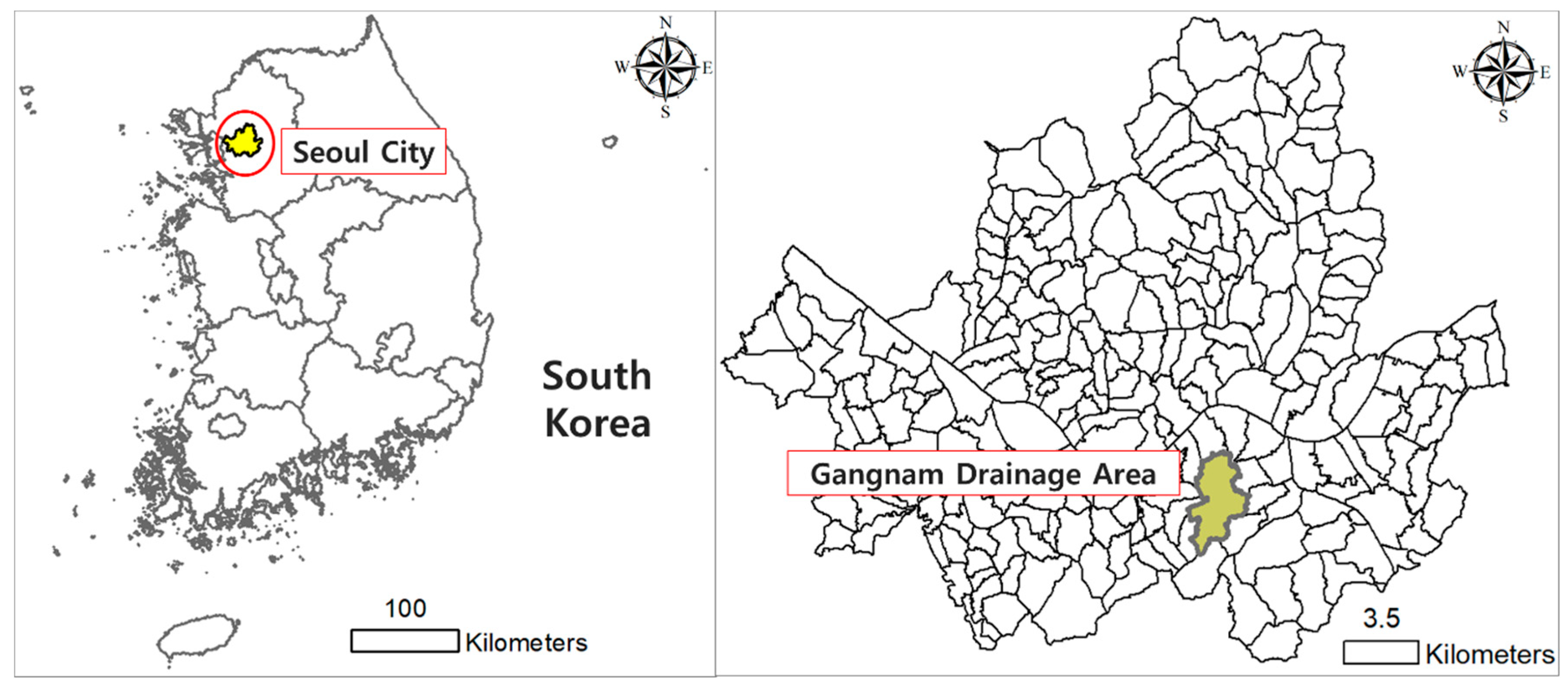
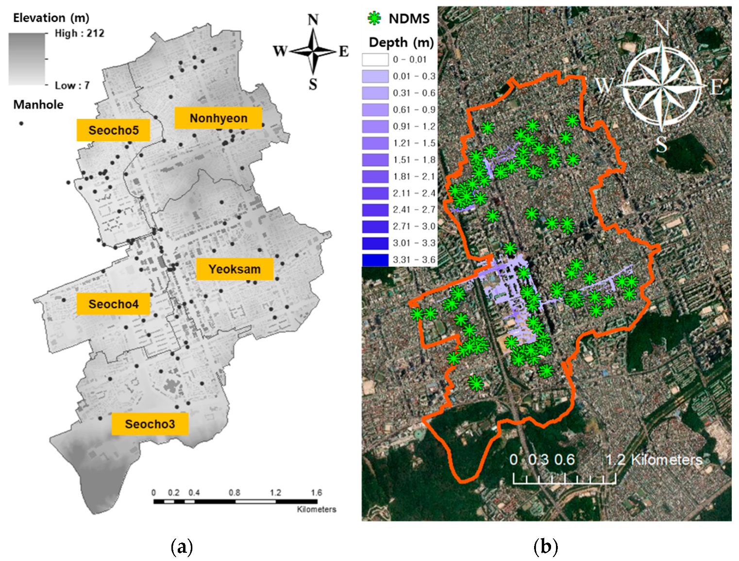
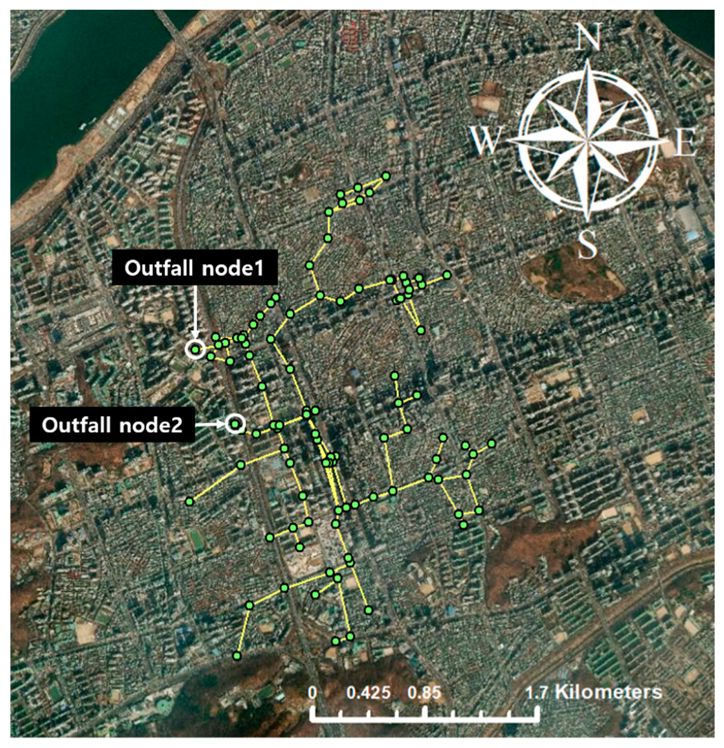
The Gangnam district in Seoul city was selected as the study area (7.4 ${\mathrm{km}}^2$). This district contains Nonhyeon, Yeoksam, and Seocho-3, 4, 5 sub-watersheds. The average annual precipitation in the study area is 1346.7 mm, the sum of precipitation in summer (June, July, August) is 808.2 mm (about 60% of annual precipitation), and the sum of precipitation in winter (December, January, February) is 55.7 mm (approximately 4% of annual precipitation). The study area consists of relatively low land in comparison with surrounding areas and has a complex drainage system, which may lead to a high risk of flooding owing to heavy rainfall [12]. In addition, this area has an inundation trace map, which shows the extent of flooding from rainfall on 21 September 2010 and 27 July 2011. The inundation area at those times was calculated as 1.4 ${\mathrm{km}}^2$ and 1.1 ${\mathrm{km}}^2$, respectively. The rainfall intensity of each rainfall event was 77.5 and 68.5 mm/hr. In 2012 and 2013, small-scale flooding occurred in the study area. Figure 1 and Figure 2 show the location of the study area and the result of a two-dimensional flood simulation using September 21, 2010 rainfall data [13]. In this study, 102 manholes and 120 conduit links were applied to a one-dimensional urban runoff simulation (Figure 3). Two outfall nodes were used, and the outfall boundary conditions were set to “free”. The free condition is an outfall stage determined by minimum critical flow depth and normal flow depth in the connecting conduit.

The simulation results were compared with NDMS(National Disaster Management System) points that indicate reporting locations during floods (Figure 2b). Verification of the two-dimensional model in the study area was conducted to indicate that the flood database in this study was reliable. For this reason, goodness of fit was calculated by counting the NDMS points that were included in the flooded area and using Equation (1) [14].

$$Goodness of Fit(\%)=\frac{Number of \mathrm{NDMS} included in the flood area}{Total number of NDMS}\times 100(\%)$$

(1)

On September 21, 2010, floods were reported by residents at 118 sites, and two-dimensional flood simulation results included 82 sites. A goodness of fit of 70.1% was estimated for the points reported by the NDMS and flood analysis results. A limitation existed due to the inability of flood flow to spread between narrow roads and buildings on account of the topographical data being processed using a 5 $\times$ 5 $\mathrm{m}$ grid. However, the goodness of fit results were deemed sufficient to produce a flood database for machine learning.

The basic data for this study consisted of the rainfall scenario probability, geographical data, and the drainage network coordinates. The probable rainfall was calculated using the return period according to the FARD2006 rainfall analysis software (National Disaster Management Institute, Ulsan, Korea). The annual maximum precipitation data recorded by the Seoul weather station during the period 1961–2015 was applied to FARD2006. Rainfall time distribution was performed with the Huff four-quantile method [15]. A total of 120 rainfall events (amount of rainfall and return period) were calculated by FARD2006 with three duration times (1, 2, and 3 hours). Rainfall data was applied to one- and two-dimensional models for generating the flood database. Geographical data based on light detection and ranging (LiDAR) data was converted to 5 $\mathrm{m}$ square digital elevation model (DEM) with consideration of road and building details. This was used as topographical data for surface flow analysis in the two-dimensional flood analysis program. The drainage network coordinates were used to accurately input the SWMM outflow results into the inflow conditions of the two-dimensional model.

The results of one- and two-dimensional analysis were applied for training neural network models. The probable rainfall (mm) was used as probabilistic neural network (PNN) and support vector regression (SVR) input data. The rainfall return period (2–100 year) was used as target data for the PNN. The flood volume (sum of 10 minutes unit overflows, ${\mathrm{m}}^3/\mathrm{s}$) calculated by the SWMM was used as target data for the SVR. The result of two-dimensional flood analysis was clustered via self-organizing map (SOM) and the SOM results were used for inundation prediction purposes. In this study, observed rainfall (mm) on September 21, 2010 was entered to train the PNN for estimation of the rainfall return period (year). Then, the estimated rainfall return period was applied to the SVR to predict flood volume (${\mathrm{m}}^3/\mathrm{s})$. The SVR flood volume and clustered two-dimensional simulation results were linked to predict the inundation map in real-time. An overall flowchart for this study is shown in Figure 4.

2.2. Numerical Model

2.2.1. One-Dimensional Runoff Analysis

In order to construct the flood prediction model, it was necessary to establish a flood database using diverse rainfall events and runoff scenarios. To calculate the runoff at each manhole in the urban watershed, the SWMM can be used with consideration of the drainage system capacity and high rainfall intensity conditions [16]. This model can consider surface and ground flows and the simulation of runoff and channel routing in an artificial drainage system [17]. This study used the EPA-SWMM because it is useful for checking the amount of urban watershed flooding.

The EXTRAN block of the EPA-SWMM can perform flow routing based on a hydraulic method with an open channel and a drainage system. A drainage system composed of pipelines connected to nodes was used to represent the physical properties and the mathematical solution for Saint-Venant’s gradual unsteady flow equation. The basic differential equation for interpreting water flow in a pipeline was derived from Equation (2), which was established by linking the momentum and continuity equations. In Equation (2), $A$ is the sectional area, $Q$ is the flow at the conduit, $V$ is the velocity of flow in the conduit, $x$ is the distance in the channel, $t$ is time, $g$ is gravitational acceleration, $H$ is the water level at the conduit, $z$ is the maximum depth of the conduit, and $S_f$ is the energy slope.

$$\frac{\partial Q}{\partial t}+gA{S}_f-2\mathrm{V}\frac{\partial A}{\partial t}-V^2\frac{\partial A}{\partial x}+gA\frac{\partial H}{\partial x}=0$$

(2)

The flood volume for each rainfall scenario was calculated by accumulating the SWMM results. Flood volume was applied as the target data for the SVR, and it also entered the two-dimensional flood analysis program as inflow data.

2.2.2. Two-Dimensional Analysis

Appropriate flood map data can be estimated by using a two-dimensional flood analysis program and a grid network that can be used for analyzing the flood flow with continuity and momentum equations. The continuity and momentum equations used are given by Equations (3)–(5). In this study, a surface flood analysis was conducted with Equations (3)–(5), which is a finite difference method [18]. The points of overflow owing to excess rainfall were treated as the inflow section, and the points where the propagated flood flow was drained were applied as the outflow section.

$$\frac{\partial d}{\partial t}+\frac{\partial q_x}{\partial x}+\frac{\partial q_y}{\partial y}=e$$

(3)

$$\frac{\partial u}{\partial t}+u\frac{\partial u}{\partial x}+v\frac{\partial u}{\partial y}=g\left(S_{ox}-S_{fx}-\frac{\partial d}{\partial x}\right)$$

(4)

$$\frac{\partial v}{\partial t}+u\frac{\partial v}{\partial x}+v\frac{\partial v}{\partial y}=g\left(S_{oy}-S_{fy}-\frac{\partial d}{\partial y}\right)$$

(5)

where $d$ is depth at a surface; $q_x$ and $q_y$ are the flows per unit width in the $x$ and $y$ directions, respectively; $\mathrm{u}$ and $\mathrm{v}$ indicate average velocities in the $x$ and $y$ directions, respectively; $S_{ox}$ and $S_{oy}$ are the bed slope $x$ and $\mathrm{y}$ directions, respectively; and $S_{fx}$ and $S_{fy}$ are the friction slopes in the $x$ and $y$ directions, respectively. The variable $e$ is the generation or extinction section per unit area. To conduct a two-dimensional flood analysis, simulated inundation results with the finite difference method were used as input data for the self-organizing map.

2.3. Machine Learning Method

2.3.1. Probabilistic Neural Network

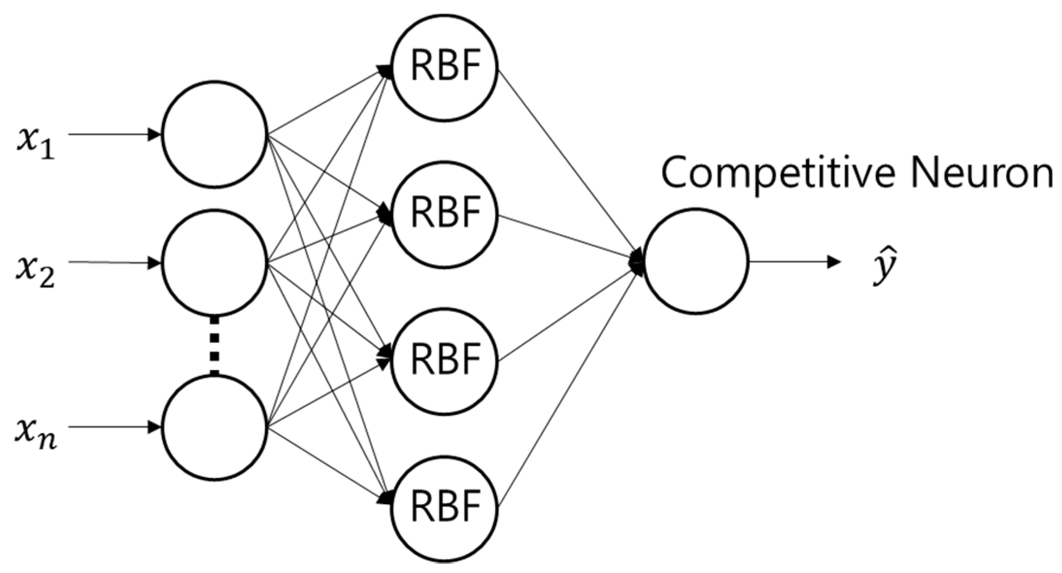
A PNN can be used for classification problems. It classifies an input vector into a specific class because that class has the maximum probability of being correct. This network has three layers: the input layer, radial basis layer, and competitive layer. The radial basis layer evaluates the vector distances between the input vector and row weight vectors in a weight matrix [19]. Distances are adjusted by radial basis function (RBF) that has a nonlinear feature, and then the competitive layer finds the shortest distance among them, thus establishing the training pattern that is closest to the input pattern based on the calculated distance. In Figure 5, $x_1$, $x_2$, …, $x_n$ are input data and $\hat{y}$ shows the estimated value. In this study, the rainfall ($\mathrm{mm})$ and duration (h) in

Table 1. Rainfall events for training of the PNN.

Return Period			Huff 1-Quartile (mm)	Huff 2-Quartile (mm)	Huff 3-Quartile (mm)	Huff 4-Quartile (mm)
1–3 h rainfall duration	2 years	1 h	48.74	48.65	48.71	48.70
		2 h	70.17	70.03	70.11	70.11
		3 h	82.78	82.62	82.71	82.71
	3 years	1 h	56.85	56.74	56.81	56.80
		2 h	82.08	81.92	82.01	82.01
		3 h	98.39	98.21	98.31	98.31
	5 years	1 h	65.96	65.83	65.91	65.90
		2 h	95.29	95.11	95.21	95.21
		3 h	115.91	155.69	115.81	115.81
	10 years	1 h	77.27	77.13	77.21	77.20
		2 h	111.91	111.69	111.81	111.81
		3 h	137.93	137.67	137.81	137.81
	20 years	1 h	88.18	88.01	88.11	88.10
		2 h	127.72	127.48	127.61	127.61
		3 h	159.05	158.75	158.92	158.92
	30 years	1 h	94.49	94.31	94.41	94.40
		2 h	136.73	136.47	136.61	136.61
		3 h	171.16	170.83	171.02	171.02
	50 years	1 h	102.19	102.00	102.11	102.11
		2 h	148.14	147.86	148.02	148.02
		3 h	186.28	185.92	186.12	186.12
	70 years	1 h	107.30	107.09	107.21	107.21
		2 h	155.65	155.35	155.52	155.52
		3 h	196.19	195.81	196.02	196.02
	80 years	1 h	109.30	109.09	109.21	109.21
		2 h	158.55	158.25	158.42	158.42
		3 h	200.19	199.81	200.02	200.02
	100 years	1 h	112.71	112.49	112.61	112.61
		2 h	163.65	163.34	163.52	163.52
		3 h	206.80	206.40	206.62	206.62

were used as input data and the rainfall return period (year) was used as target data for PNN training.

2.3.2. Support Vector Regression

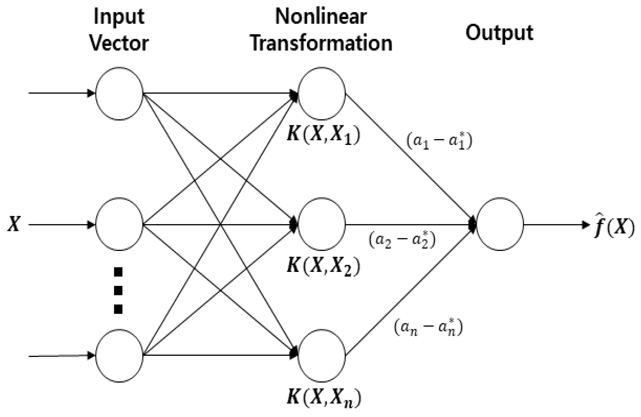
SVR was developed based on the theory of the statistical learning method [20]. The theory of the support vector machine (SVM), which was used to address the subject of classification, was extended to a regression model for prediction of continuous variance. Structural risk minimization (SRM), which minimizes the boundaries for overall errors, was recommended for machine learning rather than empirical risk minimization (ERM), which simply minimizes the difference between observed and predicted values [21]. Figure 6 shows the structure of an SVR that performs optimization using two pairs of Lagrangian multipliers ${\alpha }_i$ and ${\alpha }_i^{*}$. In the figure, $K\left(X,X_n\right)$ is the nonlinear kernel function. In this study, the input data of the SVR was the rainfall return period and the target data was flood volume as calculated by the SWMM simulation. The SVR was applied for predicting flood volume when the rainfall return period was given. In Figure 4, the variable $\mathrm{X}$ is the rainfall return period and $\hat{f}\left(X\right)$ is the predicted flood volume. The flood volume data simulated by SWMM is shown

Table 2. Flood volume database simulated by the Storm Water Management Model (SWMM).

Flood Volume Simulated by SWMM	Return Period and Duration of Rainfall		Flood Volume WithHuff 1-Quartile Rainfall (m3/s)	Flood Volume WithHuff 2-Quartile Rainfall (m3/s)	Flood Volume WithHuff 3-Quartile Rainfall (m3/s)	Flood Volume WithHuff 4-Quartile Rainfall (m3/s)
	2 years	1 h	17.82	29.36	30.16	24.46
		2 h	14.49	18.04	16.98	17.13
		3 h	12.21	14.03	13.58	12.40
	3 years	1 h	37.34	42.96	56.58	43.33
		2 h	31.65	36.25	38.95	38.20
		3 h	18.63	24.78	23.48	25.95
	5 years	1 h	55.02	89.95	101.79	88.3
		2 h	55.26	77.68	68.93	72.10
		3 h	46.48	54.22	55.76	50.58
	10 years	1 h	103.19	181.04	180.51	158.03
		2 h	116.64	149.84	148.07	147.69
		3 h	85.01	115.44	115.56	120.23
	20 years	1 h	178.17	264.05	278.16	242.56
		2 h	193.40	249.06	248.98	230.31
		3 h	164.84	221.61	214.12	217.76
	30 years	1 h	226.88	323.03	323.38	294.01
		2 h	225.46	237.56	302.01	309.70
		3 h	232.82	295.96	289.70	282.33
	50 years	1 h	319.57	389.14	387.27	340.97
		2 h	285.21	396.33	391.86	359.22
		3 h	326.11	400.23	384.11	366.27
	70 years	1 h	358.73	439.82	430.39	380.93
		2 h	368.68	462.91	449.81	412.47
		3 h	386.22	463.41	450.43	432.82
	80 years	1 h	388.84	464.98	448.29	397.73
		2 h	388.94	484.64	474.34	431.47
		3 h	411.38	489.18	484.71	455.69
	100 years	1 h	419.66	492.23	490.19	437.62
		2 h	424.95	524.40	510.35	466.06
		3 h	455.77	537.62	530.87	500.71

.

2.3.3. Self-Organizing Map

A self-organizing map (SOM) is a clustering technique based on unsupervised learning. This can be trained even if it is not given a target vector. The representative vector for each cluster is stored as weight for the corresponding output neurons [22]. The numerical distance relationship on the input space is maintained in the two-dimensional lattice space of the output neurons. The structure of an SOM is shown in Figure 7 and the data features are expressed by maintaining the intact topological attributes. In this study, the SOM input data consisted of inundation maps that were simulated via two-dimensional flood analysis modeling. The total number of inundation maps, 120, was the same as the number of rainfall scenarios. In

Table 3. Maximum flood area of SOM input data inundation map.

Rainfall Scenario		Duration	$\mathbf{Max}. \mathbf{Flood} \mathbf{Area} \left(\mathbf{k}{\mathbf{m}}^2\right)$	Rainfall Scenario		Duration	$\mathbf{Max}. \mathbf{Flood} \mathbf{Area} \left(\mathbf{k}{\mathbf{m}}^2\right)$
Two-dimensional simulation results	2 years	1 h	0.085	Two-dimensional simulation results	30 years	1 h	0.565
		2 h	0.086			2 h	0.604
		3 h	0.083			3 h	0.566
	3 years	1 h	0.174		50 years	1 h	0.638
		2 h	0.118			2 h	0.696
		3 h	0.106			3 h	0.638
	5 years	1 h	0.333		70 years	1 h	0.679
		2 h	0.307			2 h	0.769
		3 h	0.249			3 h	0.728
	10 years	1 h	0.436		80 years	1 h	0.702
		2 h	0.477			2 h	0.785
		3 h	0.402			3 h	0.746
	20 years	1 h	0.523		100 years	1 h	0.724
		2 h	0.566			2 h	0.823
		3 h	0.539			3 h	0.746

, the widest inundation area among the four Huff quantiles is indicated by the rainfall return period. The SOM results are clustered inundation maps, and the results were used as expected inundation maps. The output dimensions were set as 4 $\times$ 4 (16), 5 $\times$ 5 (25), and 6 $\times$ 6 (36) by reference to the research of [10]. The clustered inundation map that has a flood amount similar to the SVR prediction results (via SOM results) was selected and, finally, the inundation map prediction was performed through correction using interpolation.

3. Applications

3.1. Observed Rainfall for Testing Suggested Methodology

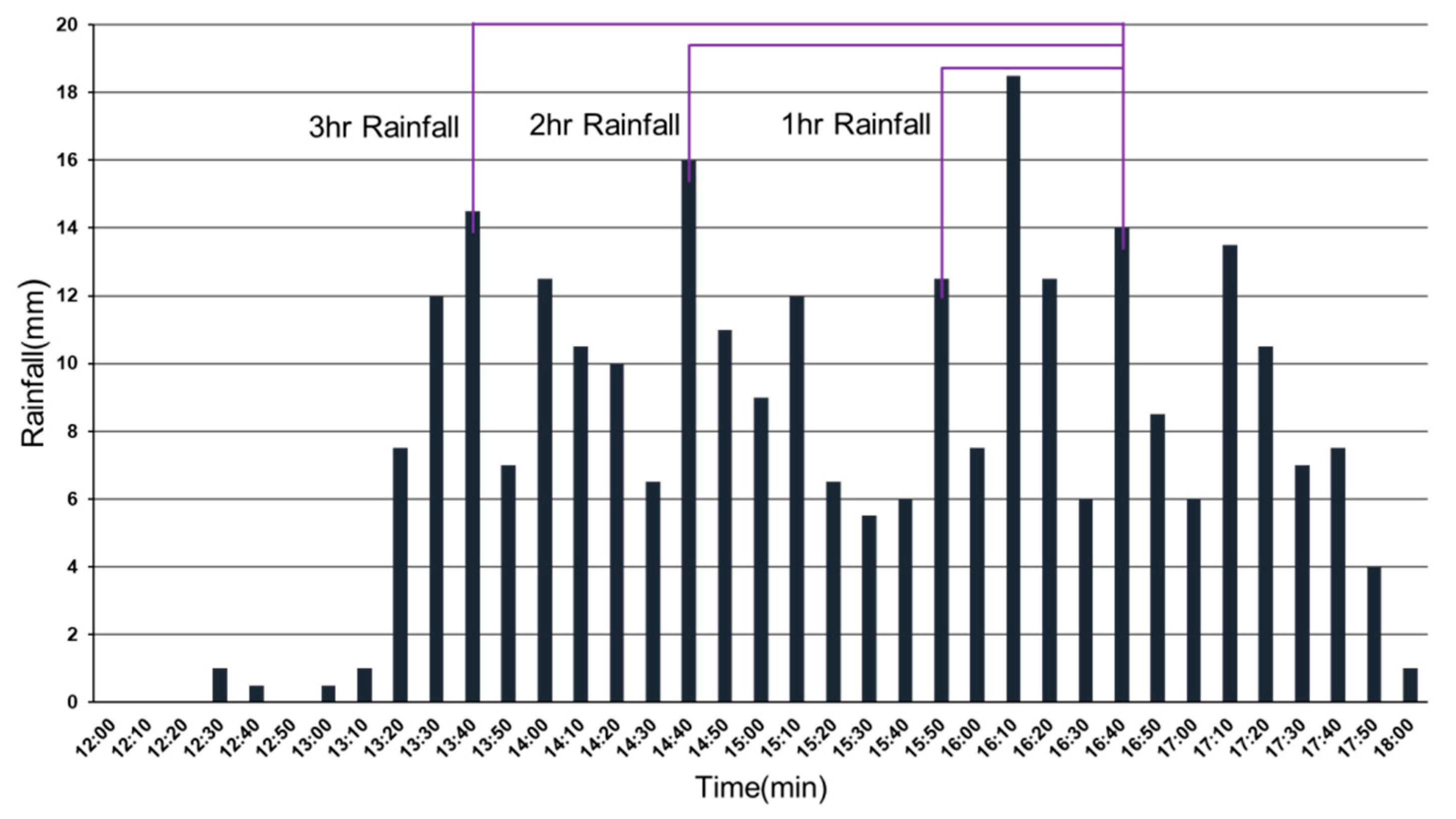
The purpose of this study was to estimate the rainfall return period with consideration of rainfall duration, and to predict a flood map for observed rainfall on 21 September 2010 (Figure 8). The rainfall data that was obtained from the Automatic Weather System (AWS) in Gangnam, and rainfall between 12:00 to 18:00 were selected. In this study, the rainfall events containing peak rainfall values for each time duration were used as target data. The rainfall durations for the prediction and simulation were set as 1, 2, and 3 h. Total rainfall was 71 mm for the duration of 1 h, 128.5 mm for 2 h, and 204 mm for 3 h.

3.2. SOM Results

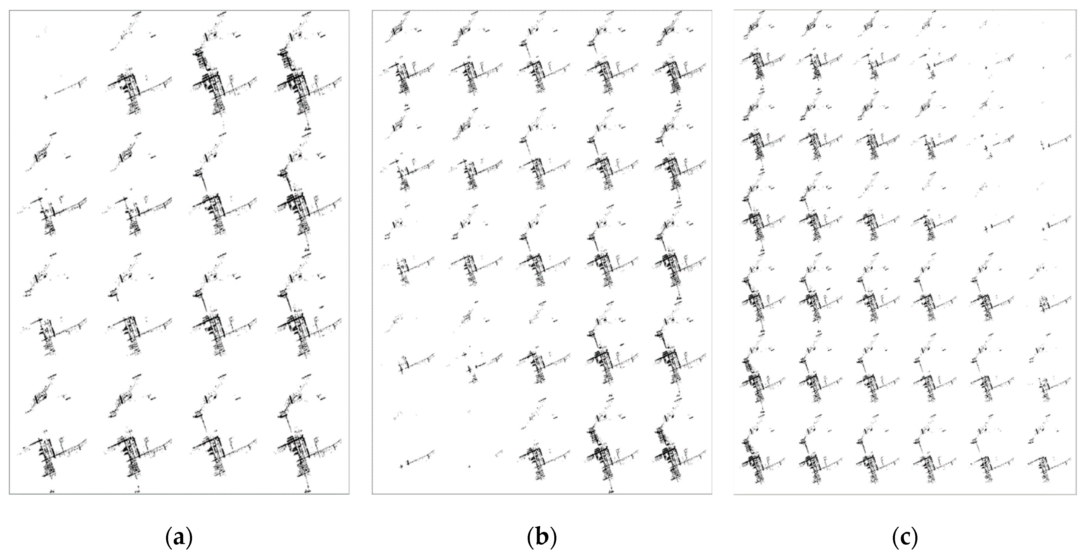
As shown in Table 2, the results of the two-dimensional hydraulic analysis were used as SOM input data. This makes it possible to reflect various flood patterns when implementing inundation predictions. It is unrealistic to check all possible time intervals of an inundation map when prediction is performed. Therefore, it is necessary to reduce the amount of expected inundation data in order to implement prediction in real time. For this reason, SOM was applied to produce 16 (4 $\times$ 4), 25 (5 $\times$ 5), and 36 (6 × 6) inundation maps (Figure 9). To construct the SOM, the number of learning steps was 500 and a hextop topological function was used. The hextop parameter functions as a layer to internally calculate the position of neurons after arranging input data in a hexagonal pattern. Euclidean distance estimation was used to calculate the distance between neurons, and the size of the initial neighboring neuron was 3. The clustered inundation maps were used as expected inundation maps.

When flood volume is predicted by SVR, an inundation map showing the most similar flood amount is found. An expected inundation map that is similar to the predicted flood volume can be established with 16 maps of 4 × 4, 25 maps of 5 × 5, or 36 maps of 6 × 6. When an appropriate expected inundation map is found, the final predicted inundation map is displayed through adjustment using interpolation. The comparison according to which the SOM result finds the expected inundation map is to be shown later.

3.3. Rainfall Frequency and Urban Flooding

To estimate the frequency of rainfall events that caused actual flooding in the study area, observed rainfall data for September 21, 2010 was entered into the trained PNN. The observed rainfall frequency was estimated by each time duration. The estimated results were compared with the return period rainfall database used in this study (

Table 4. Results of Return Period Estimation using a Probabilistic Neural Network (PNN).

Duration	Target Rainfall (AWS data)	Comparable Rainfall in Database (1)	Comparable Rainfall in Database (2)	Estimation with PNN
1 h	71 $\mathrm{mm}$	65.$\mathrm{mm}$ (5 year return period)	77.1 $\mathrm{mm}$ (10 year return period)	10 years
2 h	128.5 $\mathrm{mm}$	127.7 $\mathrm{mm}$ (20 year return period)	136.4 $\mathrm{mm}$ (30 year return period)	20 years
3 h	204 $\mathrm{mm}$	200 $\mathrm{mm}$ (80 year return period)	206.4 $\mathrm{mm}$ (100 year return period)	100 years

). The return period of AWS with 1 h rainfall was estimated to be 10 years, the 2 h AWS rainfall return period was estimated to be 20 years, and the frequency of 3 h AWS rainfall was estimated to be 100 years.

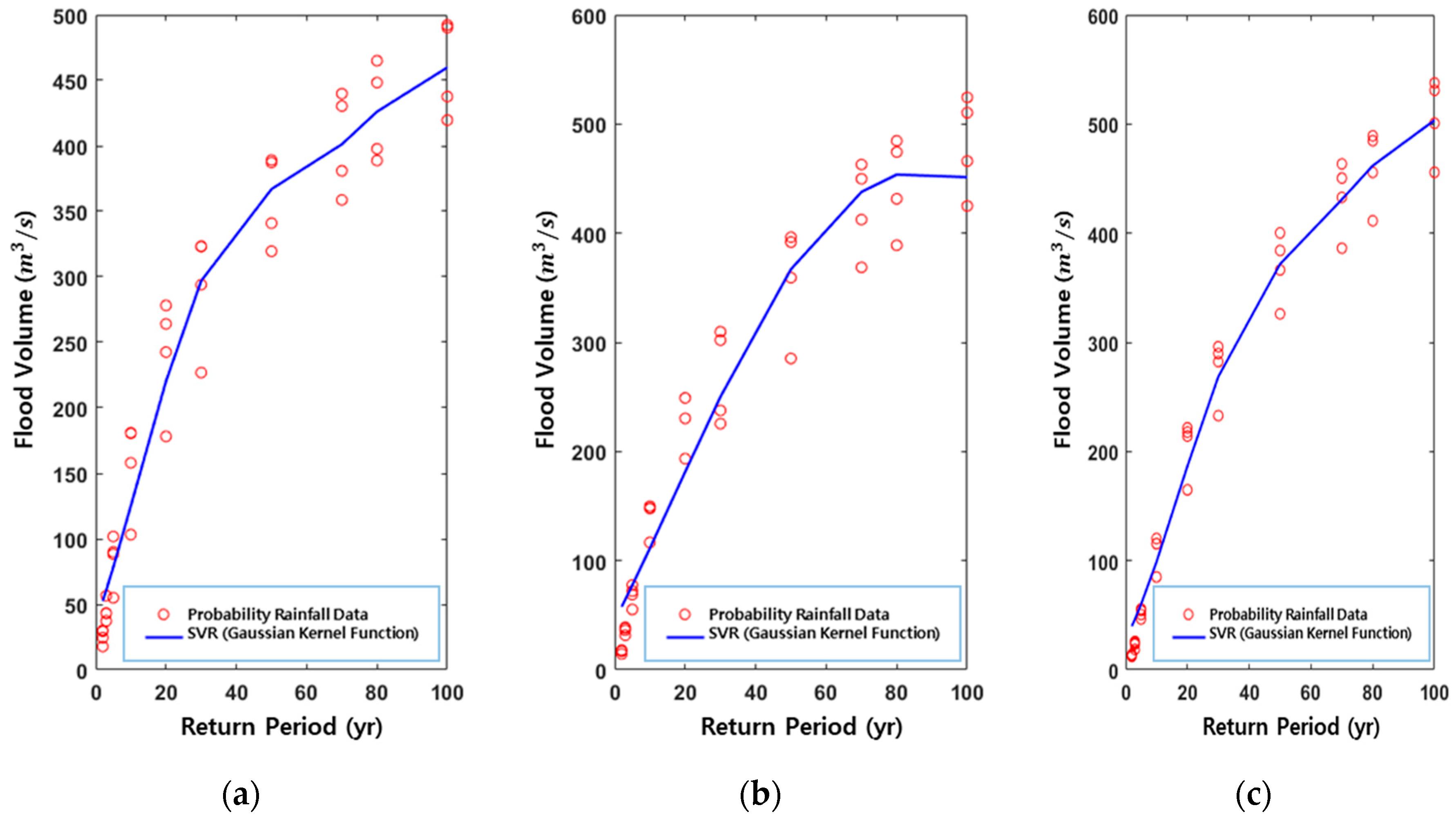
Three kernel functions—linear, polynomial, and Gaussian—were used to train the SVR. The data for flood volume (horizontal axis) and rainfall return period (vertical axis) were entered in the SVR. Figure 10 shows the fitting result of the SVR with a Gaussian kernel function. Figure 10a shows the results of generating a regression curve (SVR) for the return period of 1 h rainfall and the SWMM simulation results. SVR curves were generated in the same way for 2 and 3 h rainfall durations (Figure 10b,c). The curves based on SVR were applied to predict flood volume with the rainfall return period estimated by the PNN. By considering PNN results (Table 4), the 10, 20, and 100 year estimated return periods were entered for predicting flood volume. The predicted flood volume according to the estimated frequency for each duration is shown in

Table 5. Flood volumes predicted using support vector regression (SVR).

Kernel Function	Rainfall Duration/ Return Period	Simulated Flood Volume (m3/s)	Predicted Flood Volume (m3/s)	Residual (m3/s) (SWMM–SVR)
Linear	1 h/10 years	145.8	258.30	−112.46
	2 h/20 years	227.5	244.37	−16.92
	3 h/100 years	469.1	289.49	179.65
Polynomial	1 h/10 years	145.8	224.66	−78.82
	2 h/20 years	227.5	225.87	1.58
	3 h/100 years	469.1	413.86	55.28
Gaussian	1 h/10 years	145.8	105.98	39.86
	2 h/20 years	227.5	217.69	9.76
	3 h/100 years	469.1	491.45	−22.31

. The residuals were calculated by subtracting the predicted flood volume results from the SWMM simulation result. As a result, it was found that the Gaussian kernel function approached the SWMM results most closely. Therefore, this predicted flood volume with the Gaussian kernel function was applied to the SOM clustering result to predict the inundation map.

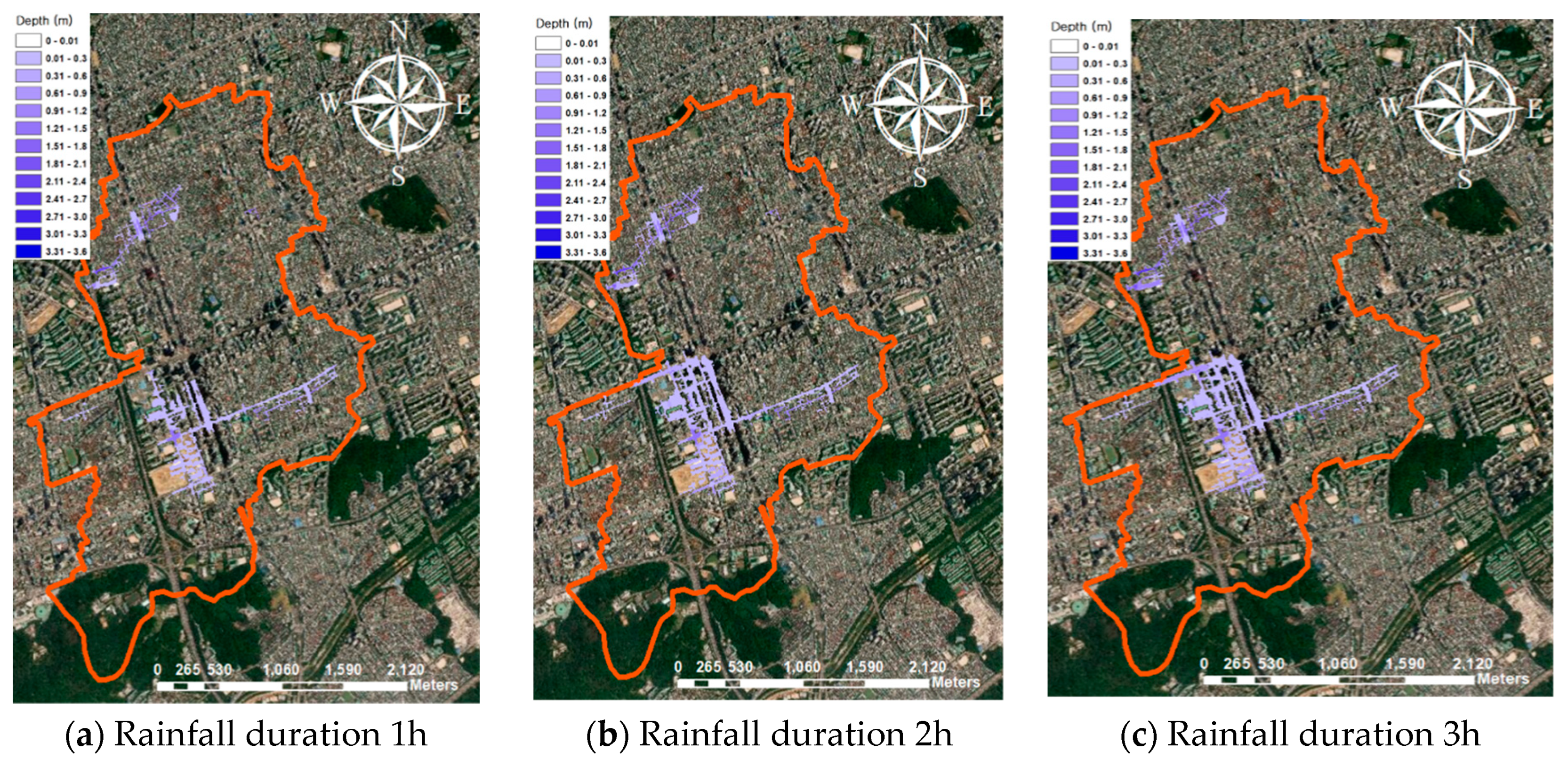
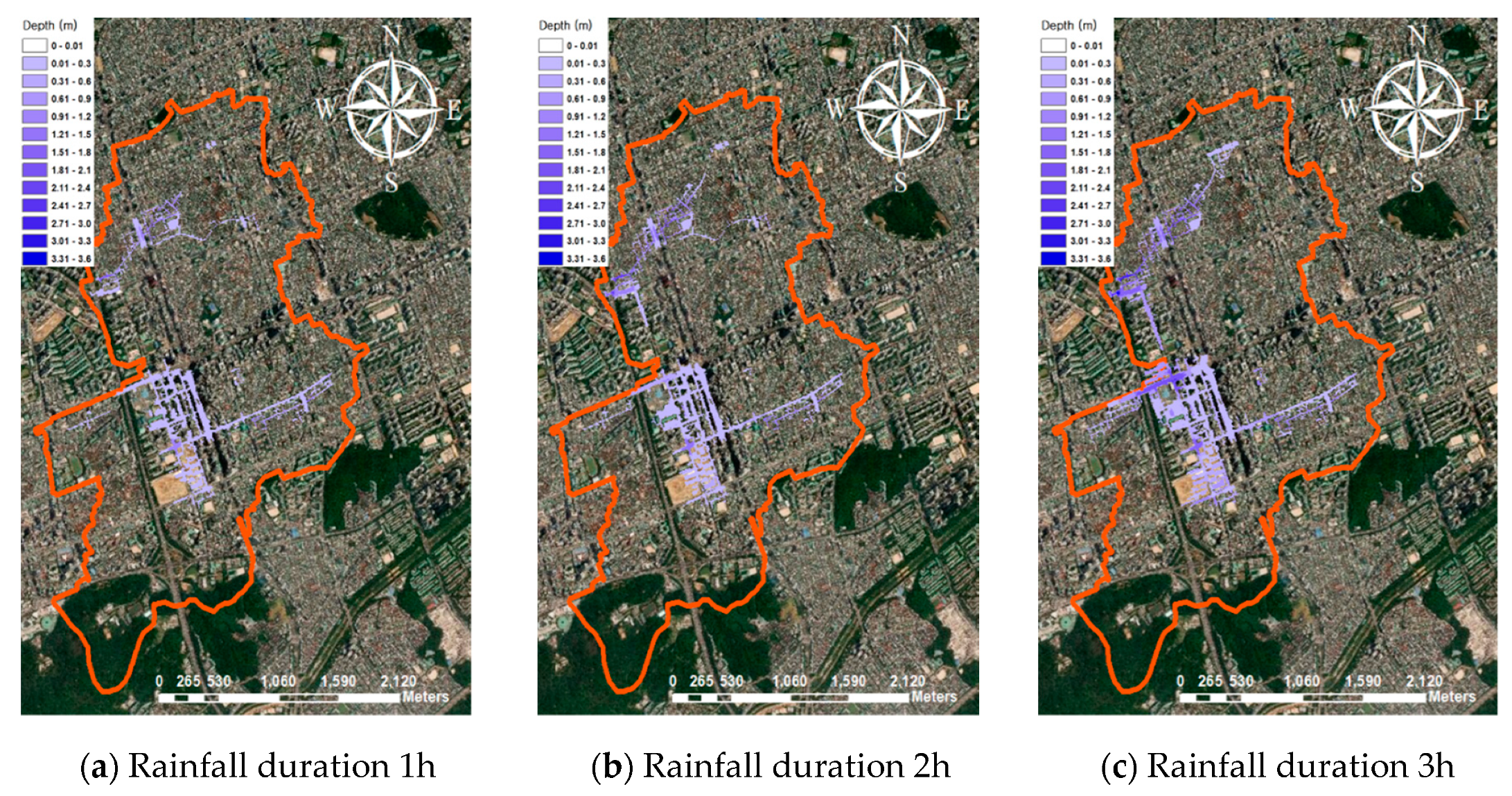
The inundation map prediction was performed by finding the similar or same flood volume among the expected inundation maps, before an adjustment process between the predicted flood volume and selected inundation map was conducted using the interpolation method. Two-dimensional hydraulic analysis with the target rainfall, used to evaluate the flood prediction results, is shown in Figure 11. The predicted inundation map obtained by linking the SVR and SOM results is shown in Figure 12. For the two-dimensional simulation shown in Figure 11, the rainfall data for each time duration in Figure 8 was used. The PNN and SVR prediction results shown in Table 4 and Table 5 were applied to the SOM results.

In order to analyze errors in the flood prediction results quantitatively, the root mean square error (RMSE), Nash sufficient efficiency coefficient (NSEC), and the goodness of fit with the flooded area were calculated by comparing with the simulated results (

Table 6. Evaluation of Flood Map Prediction.

Target Rainfall	Duration	RMSE (m)			NSEC			Goodness of Fit (%)
		SOM 4 × 4	SOM 5 × 5	SOM 6 × 6	SOM 4 × 4	SOM 5 × 5	SOM 6 × 6	SOM 4 × 4	SOM 5 × 5	SOM 6 × 6
Observed Rainfall on 21 September 2010	1 h	0.03	0.04	0.06	0.83	0.84	0.11	72.04	60.91	52.16
	2 h	0.02	0.03	0.02	0.95	0.95	0.95	81.57	81.56	85.94
	3 h	0.09	0.09	0.12	0.90	0.78	0.72	67.00	67.35	74.53

Bold text indicates the highest goodness of fit for each rainfall duration. RMSE: root mean square error; NSEC: Nash sufficient efficiency coefficient.

). RMSE and NSEC were calculated based on flood depth value. The goodness of fit is a measure of how much the inundation map prediction corresponded to the simulated flood map in grid units.

4. Conclusions

This study suggested a methodology for estimating the unknown return period of a specific observed rainfall event and for rapidly predicting an urban inundation map. The return period of observed rainfall (on 21 September 2010) was estimated through a PNN, and the flood volume and inundation map were predicted successfully by means of the estimated return period. In this study, neural network learning was performed through numerical analysis results, and various facts could be grasped via construction of a database. Flood volume simulated in urban watersheds was high when Huff’s 2nd and 3rd quartiles were mainly used. As a result of two-dimensional analysis, the inundation area with the duration of 2 hours showed the largest flood area. It is understood that rainfall in the 2nd and 3rd quartiles with a duration of 2 hours was recognized as relatively high rainfall intensity in the SWMM simulation. Finally, in order to predict flooding, it was necessary to perform a complicated process of sequentially passing through a PNN, SVR, and SOM, but it was possible to display results quickly. In addition, the inundation results were almost identical to the two-dimensional flooding analysis results. The return period of the observed rainfall was estimated using a PNN, and SVR was used to predict the flood volume considering the rainfall return period. The inundation map was predicted for the estimated rainfall return period with the PNN by linking the SVR and SOM results. The flood features for observed rainfall were successfully predicted by linking the numerical analysis model with the machine learning model. The main research results of this study were as follows:

(1)

The PNN was able to consider the return period of probable rainfall events and estimate the return period of the actual AWS event that caused flood damage in the study area. In the case of 1, 2, and 3 hours rainfall volumes recorded by the AWS on September 21, 2010, a suitable intermediate return period was estimated. Based on the presented methodology, it is possible to estimate the return period of observed rainfall, which can be used for hydrological rainfall analysis as well as flood analysis.

(2)

Flood volume prediction was performed using a trained SVR. The SVR suggested in this study was trained with quantity and return period of design rainfall events. High amounts of errors were seen when linear kernel functions were used. This was because of the nonlinearity of hydrological and flood data. However, results were greatly improved when a Gaussian kernel function was used for SVR training. When predicting the inundation map for 2 h target rainfall, the highest goodness of fit for flood area was shown to be 85.94%. Inundation prediction results for 1 and 3 h rainfall also showed more than 70% goodness of fit. Taking this result into account, the superiority of the SVR and SOM linkage model was verified. This process demonstrates that nonlinearities must be considered before predicting flood situations with machine learning methods.

(3)

The methodology suggested in this study was able to estimate the rainfall return period and predict a flood map in one process. If the flood prediction results had a high goodness of fit with results of the verified two-dimensional model, this suggests that the rainfall return period estimated by the PNN is reasonable. The results of this study can be used to inversely estimate the return period and flood volume using the predicted inundation map. This methodology could constitute the basic data for preliminary analysis of urban flooding.

References

- Pramanik, N.; Panda, R.K.; Singh, A. Daily river flow forecasting using wavelet ANN hybrid models. J. Hydroinformatics 2010, 13, 49–63. [Google Scholar] [CrossRef] [Green Version]
- Demeritt, D.; Cloke, H.L.; Pappenberger, F.; Pozo, J.T.-D.; Bartholmes, J.C.; Ramos, M.-H. Ensemble predictions and perceptions of risk, uncertainty, and error in flood forecasting. Environ. Hazards 2007, 7, 115–127. [Google Scholar] [CrossRef]
- Franz, K.; Ajami, N.K.; Schaake, J.; Buizza, R. Hydrologic ensemble prediction experiment focuses on reliable forecasts. Earth Space Sci. Newos (EOS) 2005, 86, 239. [Google Scholar] [CrossRef]
- Vojinovic, Z.; Tutulic, D. On the use of 1D and coupled 1D-2D modelling approaches for assessment of flood damage in urban areas. Urban Water J. 2009, 6, 183–199. [Google Scholar] [CrossRef]
- Domingo, N.D.S.; Refsgaard, A.; Mark, O.; Paludan, B. Flood analysis in mixed-urban areas reflecting interactions with the complete water cycle through coupled hydrologic-hydraulic modelling. Water Sci. Technol. 2010, 62, 1386–1392. [Google Scholar] [CrossRef] [PubMed]
- Cea, L.; Garrido, M.; Puertas, J. Experimental validation of two-dimensional depth-averaged models for forecasting rainfall–runoff from precipitation data in urban areas. J. Hydrol. 2010, 382, 88–102. [Google Scholar] [CrossRef]
- Bertsch, R.; Glenis, V.; Kilsby, C. Urban Flood Simulation Using Synthetic Storm Drain Networks. Water 2017, 9, 925. [Google Scholar] [CrossRef] [Green Version]
- Mosavi, A.; Ozturk, P.; Chau, K.-W. Flood Prediction Using Machine Learning Models: Literature Review. Water 2018, 10, 1536. [Google Scholar] [CrossRef] [Green Version]
- Granata, F.; Gargano, R.; De Marinis, G. Support Vector Regression for Rainfall-Runoff Modeling in Urban Drainage: A Comparison with the EPA’s Storm Water Management Model. Water 2016, 8, 69. [Google Scholar] [CrossRef]
- Chang, L.C.; Shen, H.Y.; Chang, F.J. Regional Flood Inundation Now Cast Using Hybrid Som and Dynamic Neural Networks. J. Hydrol. 2014, 519, 476–489. [Google Scholar]
- Ahn, J.; Cho, W.; Kim, T.; Shin, H.; Heo, J. Flood Frequency Analysis for the Annual Peak Flows Simulated by an Event-Based Rainfall-Runoff Model in an Urban Drainage Basin. Water 2014, 6, 3841–3863. [Google Scholar] [CrossRef] [Green Version]
- Choi, S.; Yoon, S.; Lee, B.; Choi, Y. Evaluation of High-Resolution QPE data for Urban Runoff Analysis. J. Korea Water Resour. Assoc. 2015, 48, 719–728. [Google Scholar] [CrossRef] [Green Version]
- Kim, H.I.; Keum, H.J.; Han, K. Real-Time Urban Inundation Prediction Combining Hydraulic and Probabilistic Methods. Water 2019, 11, 293. [Google Scholar] [CrossRef] [Green Version]
- Ha, C.Y.; Kim, B.H.; Son, A.L.; Han, K.Y. Accuracy Improvement of Urban Runoff Model Linked With Optimal Simulation. J. Korean Soc. Civ. Eng. 2018, 38, 215–226. [Google Scholar]
- Shin, H.S.; Ministry of Land, Transport and Maritime Affairs. Design Flood Rate Estimation with Advanced Planning Research Report; The Korea Water Resources Association: Seoul, Korea, 2010; Available online: http://www.prism.go.kr/. (accessed on 28 March 2019).
- Shin, S.Y.; Yeo, C.G.; Baek, C.H.; Kim, Y.J. Mapping Inundation Areas by Flash Flood and Developing Rainfall Standards for Evacuation in Urban Settings. J. Korean Assoc. Geogr. Inf. Stud. 2005, 8, 71–80. [Google Scholar]
- Huber, W.C.; Dickson, R.E. Storm Water Management Model, User’s Manual; US EPA: Washington, WA, USA, 1998. [Google Scholar]
- Hromadka, T.V.; Guymon, G.L.; Pardoen, G.C. Nodal domain integration model of unsaturated two-dimensional soil-water flow: Development. Water Resour. Res. 1981, 17, 1425–1430. [Google Scholar] [CrossRef]
- Wu, S.G.; Bao, F.S.; Xu, E.Y.; Wang, Y.X.; Chang, Y.F.; Xiang, Q.L. A Leaf Recognition Algorithm for Plant Classification Using Probabilistic Neural Networks. In Proceedings of the 2007 IEEE International Symposium on Signal Processing and Information Technology, Giza, Egypt, 15–18 December 2007; pp. 11–16. [Google Scholar]
- Vapnic, V.N. Statistical Learning Theory; John Wiley & Sons: New York, NY, USA, 1998. [Google Scholar]
- Chau, K.W.; Wu, C.L. Hydrological Predictions Using Data-Driven Models Coupled with Data Preprocessing Techniques; LAP LAMBERT Academic Publishing GmbH & Co. KG: Saarbrücken, Germany, 2010. [Google Scholar]
- Lopez, M.; Verdú, S.V.; Senabre, C.; Aparicio, J.; Gabaldon, A. Application of SOM neural networks to short-term load forecasting: The Spanish electricity market case study. Electr. Power Syst. Res. 2012, 91, 18–27. [Google Scholar] [CrossRef]
Figure 1.
Location of Study Area.
Figure 2.
Study area and validation. (a) Flooded Manhole; (b) Flood Simulation and National Disaster Management System (NDMS).
Figure 3.
Drainage System for one-dimensional simulation.
Figure 4.
Study flowchart.