Investigation of the Error of Mean Representative Current Velocity Based on the Method of Bins for Tidal Turbines Using ADP Data

Abstract

Representing the velocity at a tidal energy extraction site in a standardized manner is essential for the development of the tidal energy sector. The International Electrotechnical Commission (IEC) have issued a technical specification to determine the mean representative current velocity (MRV) relative to a tidal energy converter (TEC). This method determines the MRV using an acoustic Doppler profiler (ADP). This is used to evaluate the power performance of a TEC and so can have a significant influence on the power performance uncertainties, due to the cubed relationship of the MRV and power. This paper investigates these uncertainties in the MRV by considering four sources of uncertainty in the ADP. These are turbulence intensity, tilt, Doppler noise and beam misalignment of an ADP. A synthetically generated dataset is used to define current velocity and profile using the characteristics of currents and ADP. The generated synthetic dataset is processed to calculate the MRV based on the standard IEC method. An alternative method to calculate the MRV, called the temporal-spatial method (TSM), is proposed and the two methodologies are used to assess the error of the MRV. A sensitivity analysis shows that the errors of the MRV based on the standard IEC method are always higher than the TSM. The biases in the MRV based on the different combinations of the uncertainty are investigated and it is found that the bias for the MRVs based on the TSM method is generally less than that of the IEC method.

1. Introduction

The IEC has published a technical specification IEC/TS 62600-200 [1] as a guideline to assess the power performance of tidal current energy converters, which provides guidelines to determine the mean representative current velocity (MRV) at a particular location. The MRV is used for generating the power curve, which is approximately proportional to the current velocity cubed [2]. This cubed relationship means that relatively small uncertainties or errors in the MRV has a large effect on the uncertainty of power performance. Therefore, it is important to assess the uncertainty of the MRV. However, there are no studies to justify the accuracy of the MRV and its accounted uncertainties based on IEC standards. Hence, a better understanding and characterization of the uncertainties of tidal currents is essential due to the need to obtain reliable estimates of the annual energy production (AEP), which depends on the power curve during site investigations and economic projections. It is important to know the level of uncertainty and identify methods to reduce it to facilitate potential investors to predict reliable energy estimates [3]. This will lead to improvements in the accurate financial modelling of wave and tidal energy projects and provide an increased level of confidence for commercial lenders and investors.

The standard technology used for measuring the current velocity is the acoustic Doppler profiler (ADP), which is a powerful remote sensing instrument with high efficiency and reliability for probing the structure of currents and waves [4]. The method used in ADPs is Doppler effect by transmitting a signal at a fixed frequency and listening to echoes returning from the scatters in the water [5]. Thus, an ADP anchored to the seafloor can measure current speed at equal intervals from the bottom to the sea surface. Moreover, a three-dimensional velocity time series is calculated by transforming the resultant velocities using trigonometry. One of the applications of ADPs is measuring and characterization of the location’s water velocity distribution [5,6]. Thus, estimating the accuracy and uncertainties of the ADP is critical for accurate assessment of the spatial and temporal variations in the measurements [7].

The uncertainty of the MRV measured by an ADP can be influenced by many factors such as turbulence, Doppler noise, misalignment of the beam, speed of sound, moving bed, tilt of the ADP, spatial resolution, etc. [8,9]. In considering these previous studies, four sources of uncertainty in the ADP performance have been identified as the most important factors:

(1)

Turbulence intensity (TI);

(2)

Tilt;

(3)

Doppler noise;

(4)

Beam misalignment.

The turbulence intensity is considered as the ratio of the standard deviation of the velocity due to turbulence to the mean velocity, which is explained further in Section 2.1.4. Tilt is the angle between the axis of the ADP and the vertical. Doppler noise is the measurement noise of a signal which is varying with ADP configuration and flow conditions. Beam misalignment is the misalignment of beam heading of an ADP due to deviation from the nominal beam angle defined by the instrument suppliers. This can be defined as the difference between the actual vertical beam angle and the nominal beam angle (relative to vertical) of an ADP.

Kim and Yu [10] discuss the uncertainty of ADP velocity measurements for a moving vessel based on American Institute of Aeronautics and Astronautics (AIAA) uncertainty analysis standards. They proposed a mathematical framework that uses sensitivity coefficients, which supports propagation of the uncertainties of an ADP. In the 1990s and 2000s, researchers developed techniques to characterize uncertainties from turbulence intensities based on rapid samples of velocity data to estimate several turbulence parameters with the covariance technique, which addressed the bias and error sources, statistical uncertainty, and spectra [11]. A new method has been introduced to calculate the three water velocity components of a turbulent water column using autonomous underwater vehicle [12] and showed that the velocity components produced by the proposed method were within the uncertainty boundary of the ADP measurements. Presence of nonzero pitch and roll angles (tilt) create difficulties when converting beam oriented velocities, which result in errors in the current velocity measurement. In 2002, Ott introduced an alternative calculation for errors in beam velocities [13]. This involved a linear interpolation over beam velocities as a refinement for the default nearest neighbor bin-mapping algorithm. Researchers from the University of Washington and the Fraunhofer Institute have also investigated Doppler noise correction to detect estimation of the Doppler noise strength as well as turbulence intensities [14] to help understand the turbulence measurements and uncertainty budget. They found that the values for the Doppler noise estimated standard deviation are generally higher than the values suggested by manufactures, which is 0.15 m/s, although with the same order of the magnitude. However, Lu and Lueck found that the statistical uncertainty of the velocity estimates stems primarily from turbulent fluctuations rather than Doppler noise [11]. Another source of error in ADP measurements is the beam misalignment in the instrument [15]. It has been demonstrated that the beam misalignment from its nominal beam angle can cause velocity errors [16], with Woodgate and Holroyd suggesting that the actual beam angle relative to vertical can deviate by 1° or 2° [17].

The impact of instrument uncertainty on the determination of the MRV is investigated using a synthetically generated dataset. This methodology is explained in detail in Section 2. In this analysis, the error in the MRV is defined as the difference between the true MRV and the calculated MRV due to defined levels of instrument uncertainty. A set of synthetic data was generated for analysis with a predefined current profile which is considered the true velocity, together with the four sources of uncertainty from ADP measurements. This in turn allowed the testing of the IEC methodology and the new methodology with known levels of tilt, turbulence intensity, Doppler noise and beam misalignment, which facilitates the assessment of the two methodologies with respect to error and uncertainty.

The proposed methodology is developed from the existing IEC 62600-200 standard and is currently considered as the best practice for calculating the MRV. The IEC technical specification 62600-200 also provides a systematic methodology for assessing the power performance of turbines [1]. The proposed methodology, called ‘method of bins’, calculates the MRV as the power-weighted average of single point measurements across the swept area of the turbine’s rotor [18], thus, it can be summarized as a spatial-temporal averaging system where the order in which the averaging occurs first across the rotor area and then applies averaging with time. The generated synthetic data is processed to calculate the MRV and its error based on this standard methodology. An alternative method for calculating the MRV called the ‘temporal-spatial method’ (TSM) is proposed which first averages the temporal variable for each depth and then produces a power-weighted spatial average across the rotor area. The two methodologies for calculating the MRV are used to assess the error of the MRV.

The objectives of this paper are to:

(1)

Generate synthetic data using four key uncertainty parameters of an ADP as identified in literature.

(2)

Investigate the error and uncertainty of the MRV using the existing IEC standards.

(3)

Introduce an alternative method (temporal-spatial method) which reduces error and uncertainty of the MRV.

(4)

Compare the uncertainties of MRVs based on the IEC standards and the temporal-spatial method.

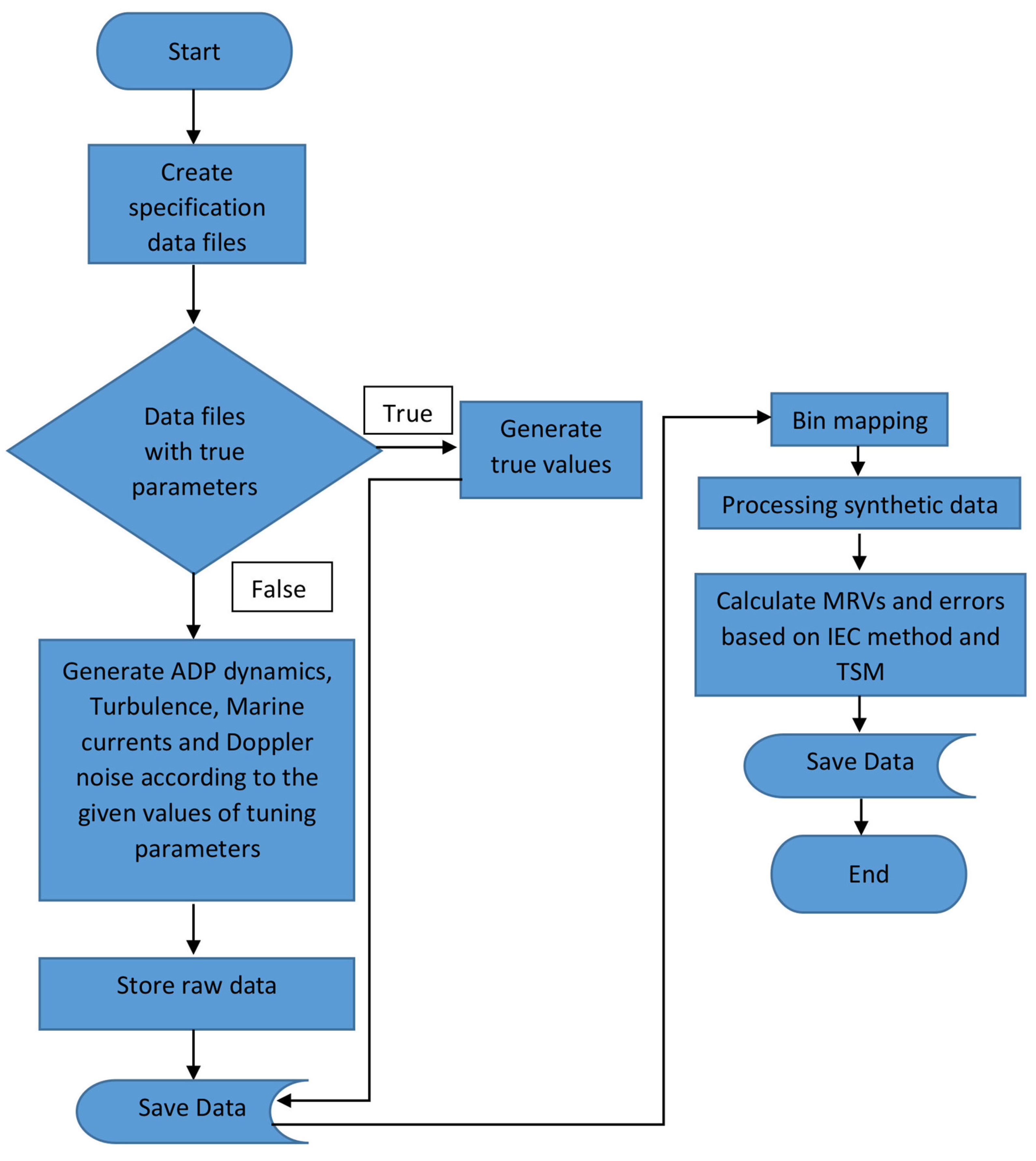
2. Synthetic Data

Synthetic datasets are used to produce estimates of the uncertainties of the processed ADP data by changing the characteristics of currents that result in uncertainty of mean velocity.

The characteristics of the currents and ADP configuration parameters used to generate the synthetic datasets are given in

Table 1. Parameters for synthetic data generation and default acoustic Doppler profiler (ADP) configuration.

Currents Characteristics		ADP Configurations
$\mathbf{Current}\mathbf{Magnitude}\mathbf{at}\mathbf{Surface},{\mathit{V}}_0$	1.0 m/s	Blanking Distance	1.0 m
Power law Coefficient, $n$	7	Height above sea bed	0.75 m
Water Depth, $d$	40.0 m	ADP beam angle, θ	20°
Current Direction	45°	Number of beams	4
-	-	Bin size	1.0 m
Sampling Duration	600s	-	-
Frequency of the Sample	2Hz	-	-

. Moreover, the standard ADP configurations which is used for this analysis are shown in Table 1.

A velocity at the surface of 1.0 m/s is used and considered to be the representative current velocity of the velocity profile. For each scenario 300 Monte-Carlo simulations were used to generate the synthetic data, which were sufficient to produce a good estimate of the expected uncertainties and errors.

The turbulence, tilt, Doppler noise and beam misalignment are defined by the four parameters; standard deviation of tilt (${\sigma }_{\delta }$), magnitude of turbulence (${\sigma }_t$), standard deviation of along-beam velocity signal due to Doppler noise (${\sigma }_n$) and standard deviation of actual beam angle (${\sigma }_{\theta })$. The true dataset is generated by assuming that there is no turbulence, no movement of the ADP, no Doppler noise and no beam misalignment, which is achieved by setting zero for all the four parameters. Different combinations of these four tuning parameters are used to generate a range of potential cases, resulting in 115 synthetic datasets as stated in Appendix A. The way of generating the scenarios is stated in

Table 2. Strategy of generating synthetic data scenarios.

Source of Uncertainty	Starting Value	Ending Value	Step Size
${\sigma }_{\delta }$	0°	10°	0.5°
${\sigma }_t$	0.0 m/s	0.3 m/s	0.01 m/s
${\sigma }_n$.	0 m/s	0.11 m/s	0.01 m/s
${\sigma }_{\theta }$	0°	1°	0.05°

.

Then two methods are used in this study to calculate the MRV—the method of bins based on IEC standards and the temporal-spatial method (TSM). It is verified that the true values were not influenced by either method used, with an analytical solution provided in Appendix B.

Figure 1 provides a flow chart of the methodology. Each synthetic dataset is generated using a Monte-Carlo simulation based on specification data files which contain the details of the hydrodynamic scenario being generated, the degree of uncertainty and variation in the hydrodynamic scenario data. The synthetic datasets are then bin mapped and processed to calculate the MRVs for the two alternative methods. Finally, a comparison is made between the MRVs based on the IEC method of bins and the TSM.

2.1. Data Generation

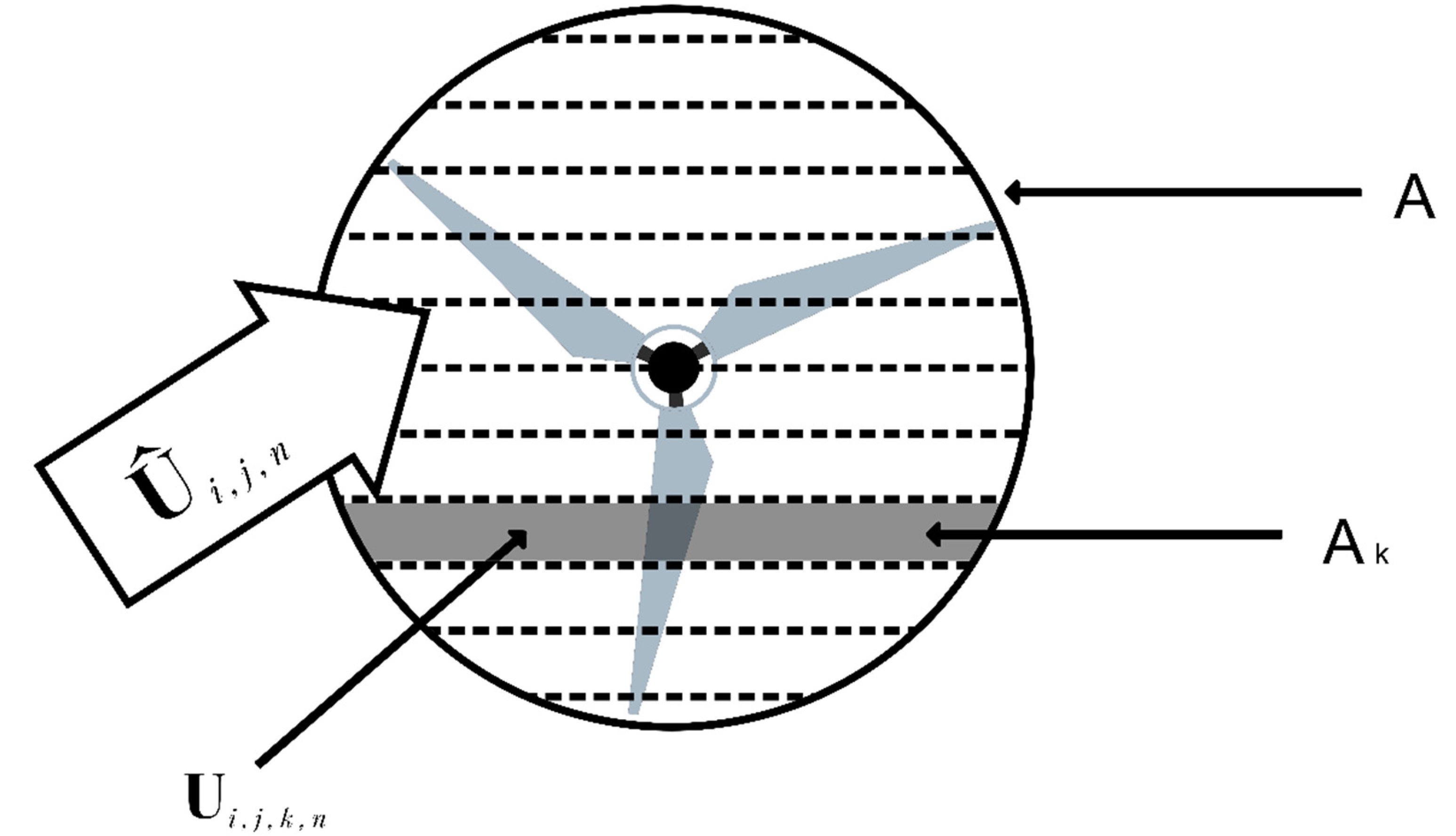
The total beam velocity can be defined as the linear sum of three components.

$$V_{tot}=V_{turb}+V_{curr}+V_{noise}$$

(1)

Movement of the ADP (or tilt) and beam misalignment result in changes to the measurement positions that are used when calculating synthetic currents in terms of the underlying current which causes different along-beam velocities. This leads to a significant impact on the total error of the MRV. Thus, the changes to the total beam velocity due to the tilt and beam misalignment are due to the use of an erroneous measurement position and thus are included in Equation (1) as $V_{curr}$.

The synthetic data generator produces estimates of the current velocity at different depths due to the tilt, turbulence, beam misalignment and Doppler noise, which are then used to calculate the MRV defined by IEC standards. The calculated representative velocities are then used to check the uncertainty of the MRV due to the four sources of uncertainty.

The following subsections provide further details on how the three different components to the measured beam velocities are calculated.

2.1.1. Currents

The current velocity profile can generally be defined using a power–law relationship between velocity and depth. Thus, the horizontal current velocities were synthetically generated as a function of depth using this power–law relationship. The typical exponent power value is considered as 1/7 in this relationship [19,20] which is used for this analysis. However it is recognized that the 1/7^th power–law is not representative of all tidal energy sites. A variation in measurement locations and beam orientation can arise due to the tilt and beam misalignment of the ADP, which causes variations in the along-beam velocities. These horizontal current velocities along with measurement position and beam orientation are then used to calculate the along-beam velocities due to currents.

The generation of the current data is based on two further standard assumptions [16], which are:

Assumption 1: At each depth the current is constant and homogenous.

Assumption 2: There is no vertical component to the current velocity.

Based on this representation, the variation of the horizontal current velocity with depth [20] is given by

$$V\left(h\right)=V_0{\left(\frac{h}{d}\right)}^{1/7}$$

(2)

To increase computational efficiency, this is calculated with a 1.0 m resolution from the seabed to the water surface. The velocity along the beam is then calculated using

$$V_{curr}=V\left(h\right)\sin \phi \cos \left(\varphi -\eta \right)$$

(3)

There is no direct perturbation of the current velocity or magnitude, but variations arise due to the tilt and beam misalignment of the ADP, which causes the measurement positions (depth) and beam orientations to change and consequently a change in the measured along-beam velocities.

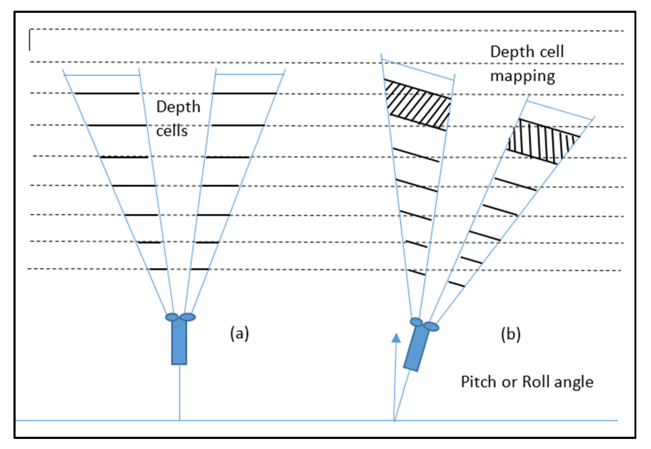
2.1.2. Pitch/Roll Movements

A potentially significant source of error in ADP measurements is movement or tilt of the ADP. It is necessary to correct the data for ADP motion to reduce this error and this process is called “bin mapping”, “depth cell mapping” or “tilt compensation” and is illustrated in Figure 2. The errors during the procedure depend on the degree of the tilt and also the method used for bin mapping [19]. The standard linear interpolation technique [13] is used as the bin-mapping method in this study.

Changes in pitch and roll angles of an ADP due to its movement affect the along-beam velocities [21]. Different amounts of pitch/roll are modelled to represent the movement of the ADP assuming that the pitch and roll are uncorrelated. The standard deviation of both the pitch and roll is varied from 0° to 10° to investigate the effect of ADP movement on the along-beam velocity.

For a particular bin, the beam velocities are expressed when defining the local reference frame as positive towards the ADP as in Equation (4), which is illustrated in Figure 3.

$$\begin{array}{c}{V}_1=V_{hx}\sin \left({\theta }_0-\alpha \right)-V_v\cos \left(\theta -\alpha \right)\\ V_2=-V_{hx}\sin \left({\theta }_0+\alpha \right)-V_v\cos \left(\theta +\alpha \right)\\ V_3=-V_{hy}\sin \left({\theta }_0-\beta \right)-V_v\cos \left(\theta -\beta \right)\\ V_4=V_{hy} \sin \left({\theta }_0+\beta \right)-V_v\cos \left(\theta +\beta \right)\end{array}$$

(4)

It is found that effect of pitch and roll can be combined as the tilt angle defined as the angle of the ADP axis relative to vertical (Appendix C).

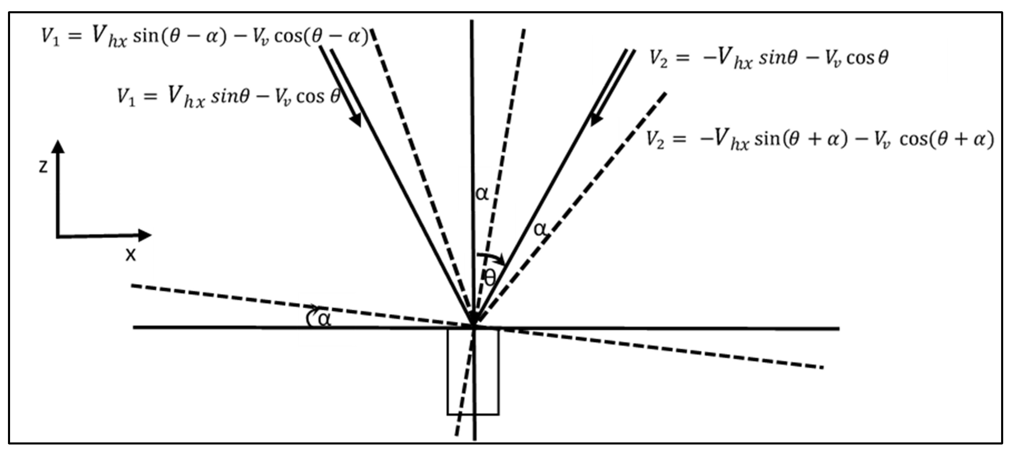
2.1.3. Beam Misalignment

Misalignment of a beam heading of an ADP is a deviation from the beam angle defined by the instrument suppliers, typically due to limitations in the ADP manufacturing process. Typical commercially available ADPs have nominal beam angles of between 20° to 30°. Therefore, it is important to study the beam angle misalignment and its influence on the uncertainty of ADP measurements.

In this study, the beam misalignment is kept constant for each simulation and generated using a random set of beam angles at each beam with a normal distribution given by

$$\theta =normal\left( {\mu }_{\theta }, {\sigma }_{\theta }\right)$$

(5)

Here, the mean value ${\mu }_{\theta }$ is the nominal beam angle of the ADP (i.e. 20°), so that the deviation of beam angle from its defined value due to beam misalignment can be generated by adjusting ${\sigma }_{\theta }$ at different levels. The values used for ${\sigma }_{\theta }$ for this study range up to 1° as suggested by Woodgate and Holroyd [17].

2.1.4. Turbulence

Turbulence is a random process, which is defined as the standard deviation of along-beam instantaneous velocity. The analysis assumes that the turbulence is isotropic and so unaffected by the beam tilt or orientation. However, turbulence has some spatial coherence and so the correlation between bins that are close together needs to be considered. To produce an estimate of this correlation, a real ADP dataset is used to identify the statistical characteristics of true instantaneous velocities due to turbulence. This real dataset was taken from an RD Instruments Workhorse ADP deployed at a potential tidal turbine deployment site in Northern Ireland. The proposed TEC for the site has a 12 m hub height and 15 m diameter horizontal axis rotor. The identified statistical characteristics are then used to generate synthetic instantaneous velocities due to turbulence. It is assumed that the instantaneous velocities due to turbulence shares the same statistical qualities with a “white noise” frequency spectrum, which has no correlation between time steps. The velocities induced by turbulence are based on the following assumptions:

Assumption 1: The time-averaged vertical flow velocity is zero for all bins.

Assumption 2: The azimuthal angle between two beams is 90°.

$$\begin{array}{c}{V}_{b12}\left(t\right)=V_{t12}\left(t\right)+V_{h12}\sin \left(\theta \pm \alpha \left(t\right)\right)\\ V_{b34}\left(t\right)=V_{t34}\left(t\right)+V_{h34}\sin \left(\theta \pm \beta \left(t\right)\right)\end{array}$$

(6)

The proximity of the correlation of bins’ instantaneous velocity can be expected due to the size of the turbulence structure. Therefore, adjacent bins’ correlations between sets of instantaneous velocity due to turbulence are calculated and the relevant estimated correlation matrix of the Pearson’s correlation coefficients is created using the Choleskey decomposition method. This guarantees that the desired variable has the same statistical properties as the real instantaneous velocities due to turbulence. The adjacent bins’ correlation coefficients of the measured correlation matrix were inspected to identify a pattern in neighboring bins of instantaneous velocities due to turbulence. The appropriate correlation matrices for adjacent bins’ instantaneous velocity due to turbulence were identified as in

Table 3. Estimated correlation matrix for instantaneous velocity due to turbulence using the recognized pattern of adjacent bins’ correlation of measured data.

Bin	Bin1	Bin2	Bin3	Bin4	Bin5	Bin6	Bin7
Bin1	1	0.4	0.25	0.2	0.15	0.1	0.05
Bin2		1	0.4	0.25	0.2	0.15	0.1
Bin3			1	0.4	0.25	0.2	0.15
Bin4				1	0.4	0.25	0.2
Bin5					1	0.4	0.25
Bin6						1	0.4
Bin7							1

below. It was found that there was no correlation in velocity between beams and bins that were separated by more than six bins where the correlation matrices for all four beams are approximately equal. Thus, the correlation coefficient where no correlation found between bins was set to zero.

The instantaneous velocities for each bin can then be generated using the Cholesky decomposition as described in the steps below. First, it is necessary to define the covariance matrix ${\displaystyle \sum }$ using the relationship of correlation–covariance.

$$R_{est}=\frac{{\displaystyle \sum }}{{\sigma }_t{\sigma }_t}$$

(7)

Then, the instantaneous velocity due to turbulence can be generated using the following equation.

$${\displaystyle \sum }={\sigma }_t{R}_{est}{\sigma }_t$$

(8)

The desired variable for instantaneous velocity due to turbulence is estimated using the Choleskey decomposition methodology.

$$V_{turb}=normal\left(0,{\displaystyle \sum }\right)$$

(9)

Different values for the standard deviation of the velocities ${\sigma }_t$ are modelled to achieve turbulence from 0.0 (as the true condition with no turbulence) to higher levels of up to 0.3 m/s to investigate the change in along-beam velocity due to the magnitude of turbulence.

This study investigates turbulence intensities (TI) ranging from 0%–30%, which is defined as the ratio of the standard deviation of the velocity to the mean velocity [22,23] where in this case the mean velocity is defined as the velocity at the hub height.

$$TI=\left(\frac{{\sigma }_t}{V_{hub}}\right)100\%$$

(10)

2.1.5. Doppler Noise

An ADP measures the Doppler-shift in frequency between transmitted pulse and the reflected pulse form the water particles. Thus, Doppler-shift measurement errors occur when measuring beam velocities, and these random errors are called Doppler noise [23]. The magnitude of the Doppler noise depends on the ADP configuration, acoustic frequency and bin size.

Doppler noise results in a measured velocity with a zero mean and a normal distribution that changes with each time step as it is a random process which has the characteristics of white noise with a Gaussian distribution [24].

$$V_{noise}=normal\left(0, {\sigma }_n\right)$$

(11)

Doppler noise levels from zero up to a theoretical Doppler noise level of 0.11 m/s [14,25] are modelled to investigate the influence of Doppler noise.

3. Processing Data

Synthetically generated data is used to investigate the calculation of the MRV based on IEC/Technical Specification (TS) 62600-200 which provides guidelines to determine the MRV to assess the power performance of TECs. Furthermore, an alternative method also used to calculate the MRV by reversing the averaging order of the methodology is provided in the IEC standards. These calculated values are used to make a comparison between MRVs based on both methods to assess the performance of each method in terms of uncertainty.

3.1. MRV Based on IEC Standards (Methoof Bins)

The IEC technical specification for power performance assessment of tidal energy converters defines the standards of calculating current velocity and performing power curve, which can be derived using the method of bins. The method of bins can be summarized as a spatial-temporal averaging system as illustrated in Figure 4 where the order in which the averaging occurs across the rotor area first and subsequently averaging with time.

The method can be summarized as follows:

Step 1: Calculate instantaneous power weighted current velocity (${\widehat{U}}_{j,n}$) across the projected captured area using the magnitude of the instantaneous current velocity ($U_{i,j,n})$.

The IEC/TS 62600-200 standards state that the representative velocity used to define the power curve for a tidal turbine is given by

$${\widehat{U}}_{j,n}={\left[\frac{{{\displaystyle \sum }}_{i=1}^s{U}_{i,j,n}^3·A_i}{{\displaystyle \sum }{A}_i}\right]}^{\raisebox{1ex}{$1$}\!\left/ \!\raisebox{-1ex}{$3$}\right.}$$

(12)

The summation of the product of cubed value of $U_{i,j,n}$ for each bin and the swept area of the corresponding bin is calculated and its cube root is taken to provide ${\widehat{U}}_{j,n}$.

Step 2: Calculate the temporal average of ${\widehat{U}}_{j,n}$ to identify the mean power weighted current velocity (or MRV,$\overline{U_n}$).

The mean power weighted current velocity $\overline{U_n}$ is calculated by taking the cube root of the temporal average of cubed values of ${\widehat{U}}_{j,n}$ over L time steps as follows;

$$\overline{U_n}={\left[\frac{ 1}{L} {\displaystyle \sum }_{j=1}^L{\widehat{U}}_{j,n}{}^3\right]}^{1/3}$$

(13)

3.2. Temporal-Spatial Method(TSM) for Calculating MRV

As shown, the IEC technical specification 62600-200 is structured so that effectively it first involves a spatial integral followed by a temporal mean. However, because the velocity is power-weighed, this has the effect of power-weighting any “noise”, which then influences the temporal mean. The TSM introduced in this paper is an alternative to the IEC standard method that reverses the order of calculation. Thus, the temporal-spatial method is calculated by first averaging the temporal variable for each depth and then the power-weighted spatial averaging across the rotor area to obtain the MRV.

The new method of calculating the MRV can be summarized as follows.

Step 1: Calculate the temporal-averaged current velocity for each bin ($\overline{W_{i,n}}$) using the magnitude of the instantaneous current velocity ($U_{i,j,n}$).

The $\overline{W_{i,n}}$ values were calculated by taking the average of cubed $U_{i,j,n}$ for L time steps and then calculating the cube root of overall value.

$$\overline{W_{i,n}}={\left[\frac{ 1}{L} {\displaystyle \sum }_{j=1}^L{U}_{i,j,n}{}^3\right]}^{1/3}$$

(14)

Step2: Calculate mean power weighted current velocity (MRV, $\overline{W_n}$) using temporal-averaged current velocity.

The mean power weighted current velocity $\overline{W_n}$ is calculated by considering the $\overline{W_{i,n}}$ values with the same power weighted method across the projected captured area, which is used in IEC/TS 62600-200 standards, but in this method, temporal-averaged current velocity for each bin ($\overline{W_{i,n}}$) is used with corresponding swept area ($A_i$) instead of using the magnitude of the instantaneous current velocities ($U_{i,j,n}$).

$$\overline{W_n}=\left[\frac{{{\displaystyle \sum }}_{i=1}^s {\overline{W_{i,n}}}^3·A_i}{{\displaystyle \sum }{A}_i} \right]{ }^{\raisebox{1ex}{$1$}\!\left/ \!\raisebox{-1ex}{$3$}\right.}$$

(15)

4. Results

The Results section focuses on investigating the error in the MRV due to the four uncertainty factors, which have been identified as major factors that may contribute to the uncertainty of the MRV. The two methodologies for calculating the MRV which were explained in Section 3 are used to evaluate the error of the MRV.

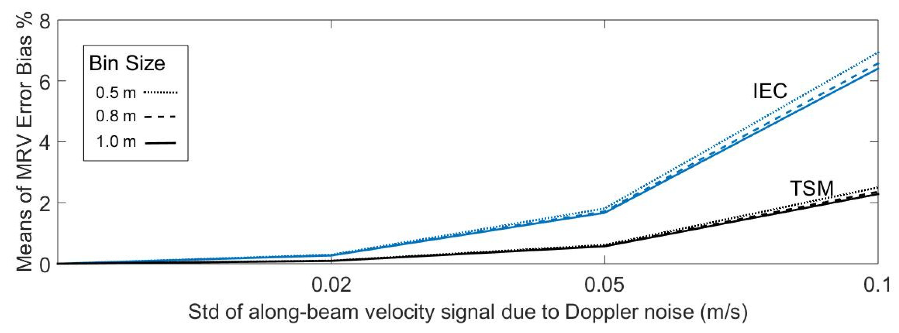
4.1. Selecting Bin Size to Reduce MRV Error due to Doppler Noise

Doppler noise has been identified as one of the major contributed uncertainty factors of the MRV. The main factors affected to Doppr noise are sampling rate and the bin size, which are related to temporal and spatial resolution, respectively [26,27]. There is a compromise between bin size and Doppler noise of an ADP since the Doppler noise of individual pings can be reduced by using larger bins which drops the Doppler noise significantly. Thus, the bin size also effects the error of the MRV due to Doppler noise. Therefore, it is generally accepted to use larger bins which reduce the Doppler noise and eliminate large raw turbulence intensities [25]. Figure 5 illustrates the means of MRV error bias as a result of change in standard deviation of long-beam velocity signal due to Doppler noise. It shows the variation in error bias of the IEC method and the TSM with three different bin sizes at 0.02, 0.05 and 0.1 standard deviation.

The bin size picked as 1.0 m to reduce the amount of the noise for the synthetic data generation in this study. In Figure 5, the means of the MRV bias for the TSM are always less than the IEC bias in all the bin sizes. Regardless of the method used, the smaller bin size has greater error bias which slightly decreases in size when increasing the bin size from 0.5 m to 1.0 m. Moreover, the bias is comparatively small for the standard deviation of 0.02 m/s, whereas it is drastically increasing with the standard deviation of along-beam signal due to Doppler noise. However, the bias difference between the bin sizes is small in the TSM compared to the IEC method.

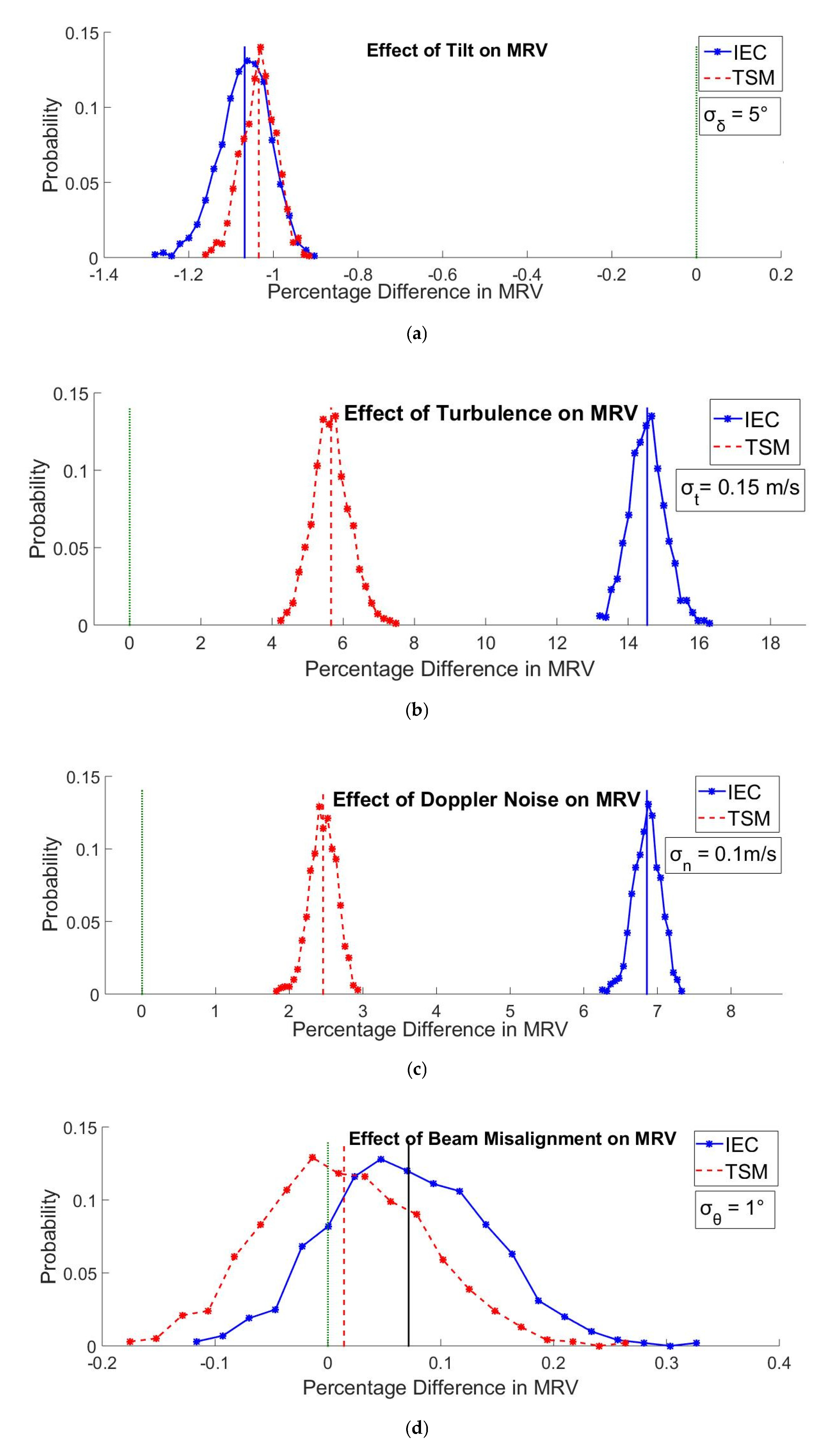
4.2. Deviations in Means of MRV with True Data

To complete an error analysis, it is necessary to define a true value. For this analysis, the true value for the MRV is considered when there is no influence of any of these factors on the data—that is there is no turbulence, tilt, beam misalignment or Doppler Noise.

The diagrams in Figure 6 show the variation of the MRV for typical values of the measurement characteristics, where the only contribution to the measurement uncertainty is the individual measurement characteristic. These results show a clear deviation of the MRV from the true value using both the IEC method as well as the TSM.

In Figure 6, the small dashed line indicates the percentage difference of means of MRV for the true MRV. It can be seen that MRV values based on either method deviate from their true value due to tilt, turbulence, Doppler noise and beam misalignment. This shows that there is an error in MRVs due to tilt, Doppler noise, turbulence and beam misalignment. For tilt, it can be seen that there is a slight deviation in MRVs from the true MRV, but the MRVs based on IEC and the TSM are relatively similar. In Figure 6b,c the effect of Doppler noise and turbulence intensity illustrate significant differences between the true MRV and the MRVs based on the two methods. The percentage difference is smaller for the MRVs based on the TSM compared to the IEC method in both Doppler noise and turbulence graphs, where the difference in means of MRVs based on two methods are 4.4% and 8.9% for Doppler noise and turbulence, respectively. There is no significant difference in MRVs due to beam misalignment even at a standard deviation of actual beam angle, ${\sigma }_{\theta }$ = 1°.

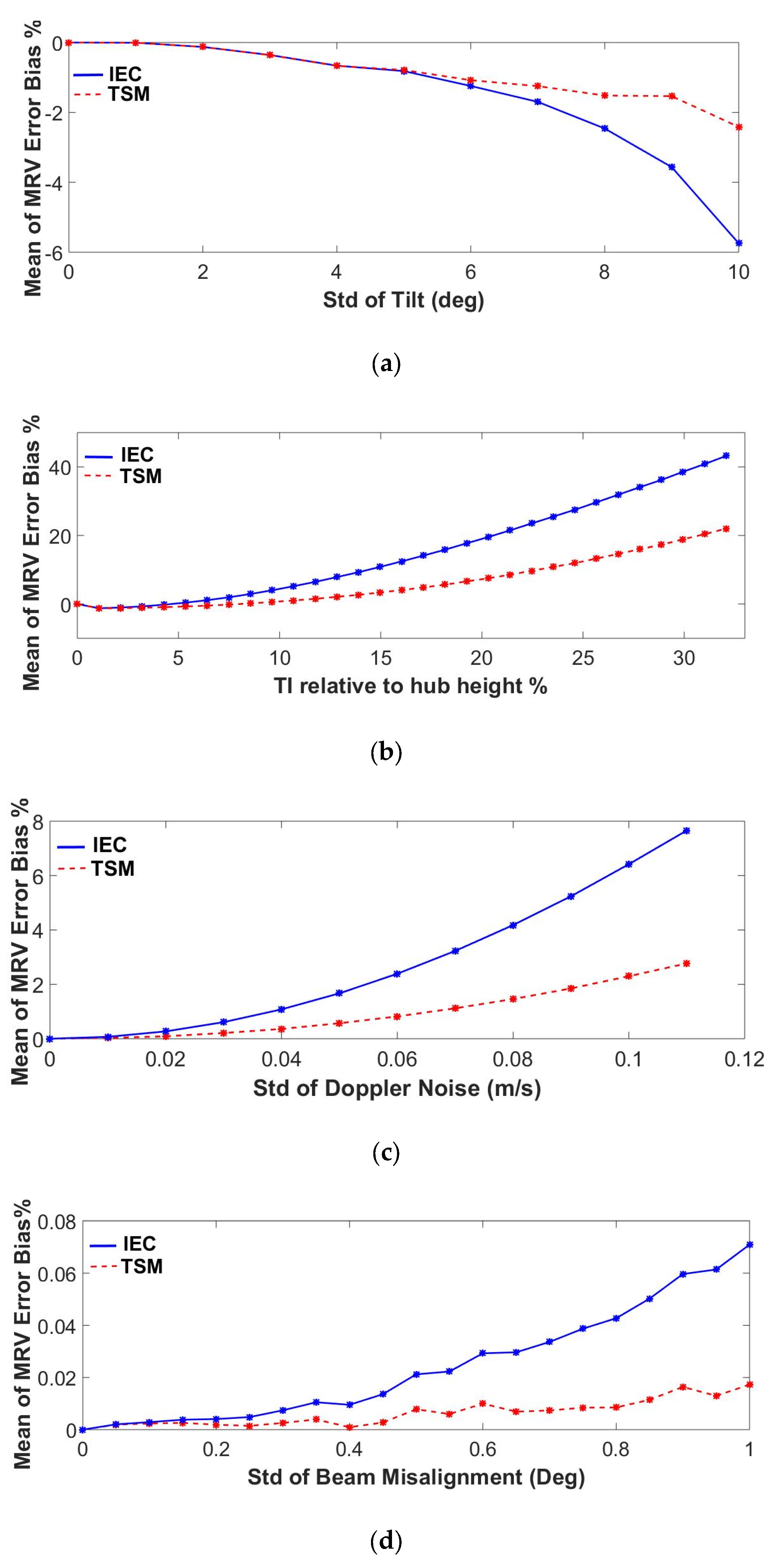
4.3. Sensitivity Analysis

The temporal-spatial method (TSM) has been shown through the sensitivity analysis to reduce the bias. A sensitivity analysis is presented in Figure 7 to assess the change in errors of means of the MRV when changing one factor at a time, and the results are indicated below using scatter diagrams.

Figure 7 shows that the TSM always has smaller errors for means of the MRV when compared to the IEC standard method. The maximum error bias can be seen in Figure 7b for TI relative to hub height, which goes up to 43.2% and 21.5% based on the IEC standard method and the TSM, respectively. Although increasing the standard deviation of tilt results in a higher error bias, the difference between errors based on both methods is negligible up to about 6°. Furthermore, the error bias due to beam misalignment is negligible where the maximum error bias is 0.07%. It can be seen that although the magnitude of the bias percentages is approximately equal for the TSM due to tilt and Doppler noise, it is slightly higher for the bias of the MRV due to Doppler noise (than tilt) based on the IEC method. This indicates that the Doppler noise influences the bias of the MRV based on the IEC method more so than the TSM.

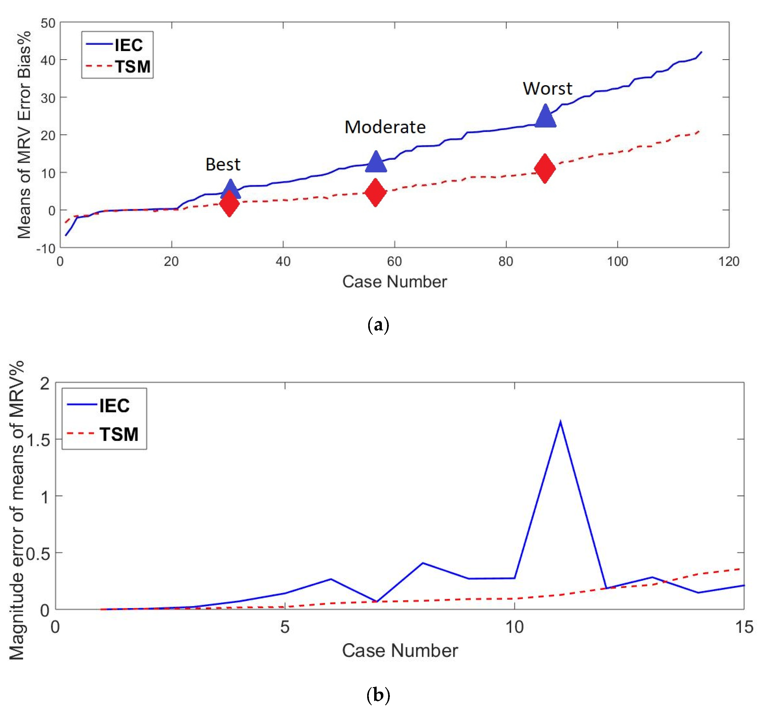
4.4. MRV Variation with Synthetically Modified Data

In this section, the results are presented to check the behavior of the MRV where the sources of uncertainty can take different combinations of values which result in various errors in the MRV. Thus, investigating the MRV variation with synthetically modified data with diverse combinations of sources of uncertainty leads to identifying the different levels of errors of the MRV with contrasting conditions. The analysis is completed for the 115 synthetically estimated means of the MRV, which were generated using Monte-Carlo simulations, to check the behavior of the MRV with random combinations of the standard deviation of tilt (${\sigma }_{\delta }$), magnitude of turbulence (${\sigma }_t$) and the standard deviation of along-beam velocity signal due to Doppler noise (${\sigma }_n$). The ${\sigma }_{\delta }$ values were changed from 0° to 10° in steps of 0.5°, whilst ${\sigma }_n$ varied from 0.00 m/s to 0.11 m/s in steps of 0.01 m/s. To produce different TI values, ${\sigma }_t$ was varied from 0.0 m/s up to 0.3 m/s with a constant increase of 0.01 m/s. However, the beam misalignment was not included due to its negligible influence on the error.

If the errors of the MRV due to each factor are uncorrelated to one another, then the variance of the sum of errors are equal to the sum of the individual variances [26,28]. Thus, the correlation coefficients are checked to assess the independence between errors of the MRV due to each factor in

Table 4. Correlation matrix for errors of means of MRV. TI: Turbulence Intensity, IEC: International Electrotechnical Commission and TSM: Temporal-Spatial Method.

Sources of Uncertainty	Noise		TI		Tilt		Misalignment
	TSM	IEC	TSM	IEC	TSM	IEC	TSM	IEC
Noise	1.000	1.000	−0.153	−0.208	−0.069	−0.097	0.004	0.006
TI	-	-	1.000	1.000	0.334	0.317	−0.090	−0.064
Tilt	-	-	-	-	1.000	1.000	0.118	0.077
Misalignment	-	-	-	-	-	-	1.000	1.000

. The correlation matrix can be displayed as follows for errors of the MRV.

It can be seen in Table 4 that all the correlation coefficients are very low, with the highest value of 0.334 obtained for the correlation between turbulence intensity and tilt. This means that the errors due to any uncertainty parameter have a minimal effect on other sources of errors. Therefore, the errors of means of the MRV due to each factor are largely independent, and since the errors in the MRV are approximately Gaussian and independent, their individual variances can be added together to produce a good estimate of the total combined error.

All the 115 synthetic data were ordered according to the ascending order of the means of the MRV to detect the variation of error bias in terms of the IEC method and the TSM, as shown in Figure 8. Three cases were selected to represent the best, moderate and worst cases by dividing the 115 ordered datasets in to three sub categories using first, second and third quartiles of the respective 115 cases. The three selected cases defined here represent the three categories where errors of the MRVs are very low, moderate or high.

The recorded error percentages for the means of the MRV based on the IEC standard method are higher than for the TSM in Figure 8. Although the two methods were conducted based on the same conditions, the errors are approximately doubled in size for the IEC standard method. However, according to Figure 8a, the IEC method produced a lower magnitude of error bias at the beginning of the distribution, whereas the TSM performed better with a lower error bias after the 15^th case. As shown in Figure 8, three cases were selected with different circumstances of magnitude of turbulence, standard deviation of tilt angle, and standard deviation of beam velocity signal due to Doppler noise to identify the change in the MRV in terms of means and standard deviations based on IEC method and TSM. These three cases were selected only for the purpose of illustrating the best, moderate and worst cases of the MRV compared with its true case. Furthermore, standard deviations of combined errors of the MRV were also calculated based on the combination of uncorrelated errors (square root of the sum of the variances) in order to check the validity of using independently generated results for the standard deviations based on Monte-Carlo simulation in

Table 5. The MRV variation due Doppler noise, turbulence and tilt at three selected levels. TI: Turbulence Intensity, MRV: Mean Representative Velocity, IEC: International Electrotechnical Commission and TSM: Temporal- Spatial Method.

Case	$\mathbf{Doppler}\mathbf{Noise}\left({\mathit{\sigma }}_{\mathit{n}}\right)$ (m/s)	TI %	$\mathbf{Tilt}\left({\mathit{\sigma }}_{\mathit{\delta }}\right)$ (Deg)	Percentage Errors of Means of MRV (m/s)		Std of MRV Based on Monte-Carlo Simulations (m/s)		Std of Combined Error of MRV Based on Variance Sum Law (m/s)
				IEC	TSM	IEC	TSM	IEC	TSM
True	0.00	0	0.0	0.000	0.000	0.00000	0.00000	0.00000	0.00000
Best	0.05	9	4.0	0.0447	0.0185	0.00333	0.00333	0.00326	0.00323
Moderate	0.10	15	3.6	0.131	0.048	0.00500	0.00520	0.00482	0.00508
Worst	0.11	23	0.5	0.329	0.157	0.00680	0.00680	0.00710	0.00692

.

The values obtained for the error in the MRV based on the Monte-Carlo simulations and the variance sum law are approximately equal in both the IEC and the TSM procedures. A significance difference can be seen between the means of MRVs based on the IEC method and the TSM. In Table 5, the error in the MRV based on the TSM is low for the worst and moderate cases and when compared with the IEC method. The worst case shows a bias in the MRV of 32.9% and 15.7% for the IEC method and the TSM, respectively.

A commonly accepted maximum error in the MRV would be 5%. According to the ordered 115 cases, only 30 cases are recorded as lower than the 5% magnitude error of the MRV based on the IEC method, whereas there are 59 for TSM. The low errors below the 5% level in both the IEC method and the TSM are found only in 30 cases. However, out of these 30 cases, only 6 cases have recorder low MRV errors based on the IEC method, while the remaining 24 errors based on the TSM are lower. Thus, some examples of combinations of TI, standard deviation of tilt angle and standard deviation of beam velocity signal due to Doppler noise are indicated as in

Table 6. Examples for acceptable combinations of uncertainty factors of MRV with 5% threshold in MRV error.

$\mathbf{Doppler}\mathbf{Noise}\left({\mathit{\sigma }}_{\mathit{n}}\right)$ (m/s)	TI%	$\mathbf{Tilt}\left({\mathit{\sigma }}_{\mathit{\delta }}\right)$ (Deg)	Bias in MRV %
			IEC	TSM
0.01	7	3.0	2.705	0.896
0.03	5	5.0	0.299	1.690
0.07	1	5.0	1.651	0.128
0.06	10	7.0	4.648	0.492
0.10	3	4.0	4.375	0.235

to guide on the 5% threshold value and the acceptable combinations of errors.

The lower error bias in the MRV can be seen for the MRV based on the TSM in Table 6, but it shows that it is not always true since the bias is sometimes lower for the MRVs based on the IEC method, and is also for the smaller values of sources of uncertainty. However, the MRV based on the TSM produces more cases below 5% error, whereas less cases with low error biases are recorded based on the IEC method.

Some applications encounter the real world expected values are shown in

Table 7. Real world examples of uncertainty factors of MRV with Doppler noise, TI and tilt.

$\mathbf{Doppler}\mathbf{Noise}\left({\mathit{\sigma }}_{\mathit{n}}\right)$ (m/s)	TI%	$\mathbf{Tilt}\left({\mathit{\sigma }}_{\mathit{\delta }}\right)$ (Deg)	Bias in MRV %
			IEC	TSM
0.11	5	5.0	7.452	2.636
0.15	5	5.0	12.387	4.686
0.11	10	5.0	10.462	3.862
0.15	10	5.0	15.238	6.002
0.11	30	5.0	38.212	18.969
0.15	30	5.0	41.744	21.171

to illustrate the bias in the MRV based on the IEC and TSM techniques.

Although the bias in the MRV of the IEC method is sometimes smaller than the TSM in Table 6, it is always higher when comparing real world examples, as in Table 7. Furthermore, the percentage change in bias is higher during the change in ${\sigma }_n$ from 0.11 m/s to 0.15 m/s without changing the other uncertainty factors, whereas it is lower when changing TI. According to Table 7, it can be observed that Doppler noise is the highly influential uncertainty factor of the MRV, rather than TI or tilt.

5. Conclusions

It can be seen that the MRV based on the TSM is always closer to the true value of the MRV than the values of the IEC standard method. This is because the MRV that has been calculated based on the standard IEC method using the power-weighted velocity which has the effect of power-weighting in error. These power-weighted errors are eliminated in the proposed alternative method by using the reverse order of the standard IEC method of calculating MRV. Thus, the errors of means of the MRV which were calculated based on the alternative method are lower than the errors obtained from the standard IEC method. The errors in the MRV due to beam misalignment are found to be small, and therefore, the influence of beam misalignment on the total means of the MRV can be assumed as negligible. The source of uncertainty that resulted in the largest errors of the MRV was found to be turbulence intensity in both the standard IEC method and the TSM. Doppler noise and tilt of the ADP have a moderate effect on the errors in the MRV. However, Doppler noise has a more significant impact on the uncertainty of the MRV than TI or tilt in real world applications. The errors of means of the MRV due to tilt, turbulence intensity and Doppler noise based on the standard IEC method are approximately double the results of those for the TSM. Due to the lack of correlation in the errors in the MRV due to each uncertainty parameter, the variance sum law can be used to provide a good estimate of the total error. Thus, the combined error in the MRV can be calculated as the square root of the sum of the variances of errors due to the individual uncertainty factor.

Although the TSM is a significant improvement over the standard IEC method, further analysis is required to identify an unbiased method to calculate MRV, which is essential to obtain a high quality power curve. Future work will utilize this proposed method to demonstrate the reduction in error with real ADP data. Furthermore, this will significantly affect annual energy production (AEP) validation, for example the accuracy and uncertainty associated with the velocity exceedance probability curve used in the IEC 62600-201. Thus the temporal-spatial method has far-reaching implications in the tidal energy community and is recommended for inclusion in the development of future standards.

References

1. Gabriel, A. Marine energy, Wave, tidal and other water current converters—Part. 200: Electricity producing tidal energy converters, Power performance assessment, IEC TS 62600-200:2013; 2013. Available online: https://www.iec.ch/dyn/www/f?p=103:23:9627634218241::::FSP_ORG_ID,FSP_LANG_ID:1316,25 (accessed on 29 May 2020).
2. Roberts, A.; Thomas, B.; Sewell, P.; Khan, Z.; Balmain, S.; Gillman, J. Current tidal power technologies and their suitability for applications in coastal and marine areas. J. Ocean. Eng. Mar. Energy. 2016, 2, 227–245. [Google Scholar] [CrossRef] [Green Version]
3. Alcérreca H., J.C.; Encarnacion, J.I.; Ordoñez-Sánchez, S.; Callejas-Jiménez, M.; Barroso Diez Barroso, G.; Allmark, M.; Mariño Tapia, I.; Silva Casarín, R.; O’Doherty, T.; Johnstone, C.; et al. Energy yield assessment from ocean currents in the insular shelf of Cozumel Island. J. Mar. Sci. Eng. 2019, 7, 1–18. [Google Scholar] [CrossRef] [Green Version]
4. González C., J.A.; Muste, M. Framework for estimating uncertainty of ADCP measurements from a moving boat by standardized uncertainty analysis. J. Hydraul. Eng. 2007, 133, 1390–1410. [CrossRef]
5. Nystrom, E.A.; Oberg, K.A.; Rehmann, C.R. Measurement of Turbulence with Acoustic Doppler Current profilers—Sources of Error and Laboratory Results. In Proceedings of the Hydraulic Measurements and Experimental Methods Specialty Conference (HMEM), Estes Park, CO, USA, 28 July 2002; pp. 1–10. [Google Scholar]
6. Gargett, A.E. Observing Turbulence with a Modified Acoustic Doppler Current Profiler. J. Atmos. Ocean. Technol. 1994, 11, 1592–1610. [Google Scholar] [CrossRef] [Green Version]
7. Laws, N.D.; Epps, B.P. Hydrokinetic energy conversion: Technology, research, and outlook. Renew. Sustain. Energy Rev. 2016, 57, 1245–1259. [Google Scholar] [CrossRef] [Green Version]
8. Muste, M.; Lee, K. WMO Project: Assessment of the Performance of Flow Measurement Instruments and Techniques. DEVELOPMENT OF THE DECISION-AID TOOL. 2012, pp. 1–45. Available online: http://www.wmo.int/pages/prog/hwrp/Flow/index.php (accessed on 26 May 2020).
9. Simpson, M.R. Discharge Measurements Using a Broad-Band Acoustic Doppler Current Profiler. United States Geol. Surv: OPEN-FILE Rep. 01–1. 2001; p. 134. Available online: https://pubs.usgs.gov/of/2001/ofr0101/text.pdf (accessed on 26 May 2020).
10. Kim, D.; Yu, K. Uncertainty Estimation of the ADCP Velocity Measurements from the Moving Vessel Method, (I) Development of the Framework. KSCE J. Civ. Eng. 2010, 14, 797–801. [Google Scholar] [CrossRef]
11. Lu, Y.; Lueck, R. Using a Broadband ADCP in a Tidal Channel. Part I: Mean Flow and Shear. J. Atmos. Ocean. Technol. 1999, 16, 1556–1567. [Google Scholar] [CrossRef]
12. Randeni, P.; Supun, A.T.; Forrest, A.L.; Cossu, R.; Leong, Z.Q.; Ranmuthugala, D. Determining the horizontal and vertical water velocity components of a turbulentwater column using the motion response of an autonomous underwater vehicle. J. Mar. Sci. Eng. 2017, 5. [Google Scholar] [CrossRef] [Green Version]
13. Ott, M.W. An Improvement in the Calculation of ADCP Velocities. J. Atmos. Ocean. Technol. 2002, 98, 173. [Google Scholar] [CrossRef]
14. Richard, J.; Thomson, J.; Polagye, B.; Bard, J. Method for identification of Doppler noise levels in turbulent flow measurements dedicated to tidal energy. Int. J. Mar. Energy 2013, 4, 52–64. [Google Scholar] [CrossRef]
15. Mueller, D.S.; Wagner, C.R. Measuring Discharge with Acoustic Doppler Current Profilers from a Moving Boat; U.S. Geological Survey Techniques and Methods 3A–22: Eston, Virginia, 2009. [Google Scholar]
16. Richmond, M.; Harding, S.; RomeroG, P. Numerical performance analysis of acoustic Doppler velocity profilers in the wake of an axial-flow marine hydrokinetic turbine. Int. J. Mar. Energy 2015, 11, 50–70. [Google Scholar] [CrossRef] [Green Version]
17. Woodgate, R.A.; Holroyd, A.E. Correction of Teledyne Acoustic Doppler Current Profiler (ADCP) Bottom-Track Range Measurements for Instrument Pitch and Roll. arXiv 2011, arXiv:1110.5003. In Press. [Google Scholar]
18. Frost, C.; Benson, I.; Elsäßer, B.; Starzmann, R.; Whittaker, T. Mitigating Uncertainty in Tidal Turbine Performance Characteristics from Experimental Testing. In Proceedings of the European Wave and Tidal Energy Conference, Cork, Ireland, 27 August 2017; p. 936(1–10). [Google Scholar]
19. Crossley, G.; Alexandre, A.; Parkinson, S.; Day, A.H.; Smith, H.C.M.; Ingram, D.M. Quantifying uncertainty in acoustic measurements of tidal flows using a ‘Virtual’ Doppler Current Profiler. Ocean. Eng. 2017, 137, 404–416. [Google Scholar] [CrossRef] [Green Version]
20. Sellar, B.G.; Wakelam, G.; Sutherland, D.R.J.; Ingram, D.M.; Venugopal, V. Characterisation of tidal flows at the european marine energy centre in the absence of ocean waves. Energies 2018, 11, 1–23. [Google Scholar] [CrossRef] [Green Version]
21. Teledyne RD Instruments Acoustic Doppler Current Profiler Principles of Operation A Practical Primer. 2011, Volume 00. Available online: https://www.comm-tec.com/Docs/Manuali/RDI/BBPRIME.pdf (accessed on 26 May 2020).
22. Garcia, N.P.; Kyozuka, Y. Analysis of turbulence and extreme current velocity values in a tidal channel. J. Mar. Sci. Technol. 2018, 24, 659–672. [Google Scholar] [CrossRef]
23. Blackmore, T.; Batten, W.M.J.; Bahaj, A.S. Influence of turbulence on the wake of a marine current turbine simulator. Proc. R. Soc. A Math. Phys. Eng. Sci. 2014, 470, 2170–2187. [Google Scholar] [CrossRef] [Green Version]
24. Nikora, V.I.; Goring, D.G. ADV MEASUREMENTS OF TURBULENCE: Can We Improve Their Interpretation? Hydraul. Eng. 1998, 124, 630–634. [Google Scholar] [CrossRef]
25. SonTek Acoustic Doppler Profiler (ADP®) Principles of Operation. 2000. Available online: https://www.sontek.com/media/pdfs/adp-brochure.pdf (accessed on 26 May 2020).
26. Lyon, V.; Wosnik, M. Spatio-Temporal Resolution of Different Flow Measurement Techniques for Marine Renewable Energy Applications. Proc. 2nd Mar. Energy Technol. Symp. METS2014 2014. Available online: https://vtechworks.lib.vt.edu/handle/10919/49225 (accessed on 26 May 2020).
27. Thomson, J.; Durgesh, V.; Richmond, M.C. Measurements of Turbulence at Two Tidal Energy Sites in Puget Sound, WA. IEEE J. Ocean. Eng. 2012, 37, 363–374. [Google Scholar] [CrossRef]
28. David, M. Lane Variance Sum Law. Available online: http://onlinestatbook.com/2/summarizing_distributions/variance_sum_law.html (accessed on 4 June 2019).
Figure 1. Flow chart of the methodology.
Jmse 08 00390 g001
Figure 2. Acoustic Doppler profiler (ADP) tilt and bin mapping (a) without tilt; (b) Processing bin mapping with the presence of tilt.
Jmse 08 00390 g002
Figure 3. Schematic for movement of an ADP. Solid lines indicate before the movement condition and dashed lines indicate after α roll angle movement of ADP for beam 1 and beam 2.
Jmse 08 00390 g003
Figure 4. Power-weighted current velocity calculation across the projected captured area illustration. Here, k is considered as index number of the current profiler bin across the projected captured area.
Jmse 08 00390 g004
Figure 5. Deviation in means of mean representative current velocity based on different bin sizes. Here, MRV: Mean Representative Velocity, IEC: International Electrotechnical Commission and TSM: Temporal-Spatial Method.
Jmse 08 00390 g005
Figure 6. MRV variation due to (a) tilt; (b) Turbulence; (c) Doppler noise; (d) Beam misalignment. Here, MRV: Mean Representative Velocity, IEC: International Electrotechnical Commission and TSM: Temporal-Spatial Method.
Jmse 08 00390 g006
Figure 7. Sensitivity study for error bias of mean of the MRV based on the TSM and the IEC method due to (a)tilt; (b) Turbulence intensity; (c) Doppler noise; (d) Beam misalignment. Here, MRV: Mean Representative Velocity, IEC: International Electrotechnical Commission and TSM: Temporal-Spatial Method.
Jmse 08 00390 g007
Figure 8. Mean of MRV error due to Doppler noise, turbulence intensity and tilt (a) for all the cases with ordered case number; (b) For 15 cases when the magnitude of the error bias is low. Here, MRV: Mean Representative Velocity, IEC: International Electrotechnical Commission and TSM: Temporal-Spatial method.
Jmse 08 00390 g008