A Framework of Numerically Evaluating a Maneuvering Vessel in Waves

Department of Ocean Engineering, Texas A&M University, College Station, TX 77840, USA
*
Author to whom correspondence should be addressed.
J. Mar. Sci. Eng. 2020, 8(6), 392; https://doi.org/10.3390/jmse8060392
Submission received: 23 April 2020
/
Revised: 27 May 2020
/
Accepted: 27 May 2020
/
Published: 29 May 2020
(This article belongs to the Special Issue Dynamic Instability in Offshore Structures)
Abstract
:Maneuvering in waves is a hydrodynamic phenomenon that involves both seakeeping and maneuvering problems. The environmental loads, such as waves, wind, and current, have a significant impact on a maneuvering vessel, which makes it more complex than maneuvering in calm water. Wave effects are perhaps the most important factor amongst these environmental loads. In this research, a framework has been developed that simultaneously incorporates the maneuvering and seakeeping aspects that includes the hydrodynamics effects corresponding to both. To numerically evaluate the second-order wave loads in the seakeeping problem, a derivation has been presented with a discussion and the Neumann-Kelvin linearization has been applied to consider the wave drift damping effect. The maneuvering evaluations of the KVLCC (KRISO Very Large Crude Carrier) and KCS (KRISO Container Ship) models in calm water and waves have been conducted and compared with the model tests. Through the comparison with the experimental results, this framework had been proven to provide a convincing numerical prediction of the horizontal motions for a maneuvering vessel in waves. The current framework can be extended and contribute to the IMO (International Maritime Organization) standards for determining the minimum propulsion power to maintain the maneuverability of vessels in adverse conditions.
1. Introduction
A ship’s maneuverability is typically only considered in calm water in most previous research [1], while a seagoing vessel maneuvering in waves is more often the actual scenario. This research on maneuvering in waves is practically significant, considering navigation safety. There are several existing methods to study ship maneuverability in waves, such as model tests and numerical simulation that can be generally classified as CFD methods, two-time scale methods, and hybrid approaches.
The experimental method is a practical and reliable methodology to investigate the ship’s maneuverability in waves. Turning circles and zig-zag tests in regular waves have been conducted to analyze various parameters such as wave length, wave direction and ship’s loading condition’s effects on maneuvering motions [2,3]. However, specific model tests are time consuming, expensive, and should only be considered for the validation of more general numerical approaches.
As for the numerical simulation, CFD methods in principle consider all physics facts but still needs further development in order to reach the level of industrial applicability. Islam et al. [4] applied an open source RANS solver, OpenFOAM to simulate hydrodynamic derivatives and his results matched well with two sets of experimental data, with the exception of the pure yaw cases. Uharek et al. [5] showed that the RANS code Neptuno was able to predict the mean drift loads for vessels maneuvering in oblique regular waves and that the inertial contributions cannot be neglected. Wang et al. [6] applied a CFD solver based on OpenFOAM and applied the overset grid technique and six DoF module to solve for the motion of the free-running ship with twin rotating propellers and turning rudders. However, CFD’s current large requirement of computational resources and technical difficulties has confined it to the research communities worldwide. The application to propellers and rudder models under large attack angle suggest that fulfillment of the real time simulation requirement is hardly to be satisfied from a realistic point of view [7]. An alternative to CFD methods are the two-time scale method and the hybrid approach, both of which are based on potential flow methods to consider the wave effect. As for the hybrid approach, it combines the maneuvering motion and wave-induced motion into the rigid body motion equations to simulate a vessel’s maneuverability [8,9], but ignores the effect of the second-order wave loads. Through the investigation by Lee et al. [10] regarding the effects of waves on ship’s maneuverability, it can be concluded that the second-order wave loads present a significant effect on the trajectory of turning and zig-zag tests. On the other hand, the two-time scale method considers and separates the ship motions into the wave frequency and low frequency components, and by doing this, it is possible to consider the second-order wave loads and motions to enhance its accuracy. Skejic and Faltinsen [11] applied the two-time scale approach to analyze ship maneuvering in regular waves, by evaluating the wave drift forces through four different strip theory methods and considering that when the ship has a mean forward speed and undertakes maneuvering in waves, the wave-frequency problem is affected by the slowly-varying maneuvering. Seo and Kim [12] developed a coupled analysis of the maneuvering and seakeeping problems through a two-time scale approach, where the wave loads were estimated using a Rankine panel method in the time domain. Lee and Kim [13] used a 3D time-domain Rankine panel method to analyze the ship motion due to the waves and near-field method to consider the wave drift loads. It can be concluded that the seakeeping quantities, such as ship motion and wave drift force, are significantly affected by both forward speed and side slip speed. Moreover, the accuracy of turning simulation results are also closely related to the prediction of wave drift loads. Chillcce and Moctar’s [14] solution assumed that the calm water hydrodynamic parameters and the wave induced forces do not interact and applied a RANS approach to obtain the calm water forces and a 3D Rankine source boundary element method to consider the wave-induced second-order loads. Their results showed that the ship’s drift in turning circle can be accurately captured by considering the mean second-order wave loads.
A derivation and full expression of the second-order wave loads acting on a floating body was presented in our previous research [15] through a direct pressure integral method, in which both the mean drift wave forces and moments coefficients and the full quadratic transfer function have been presented. It also contained a comparison of Newman’s approximation [16] with an evaluation of the off-diagonal elements in the full QTF matrix. This direct pressure integral method presented and showed the importance and necessity of considering the off-diagonal elements, especially when the difference wave frequency increases and water depth decreases. While considering the mean wave forces and moments acting on a floating body with speed, multiple numerical solutions have been proposed and applied including far field method and near field method. As for the far field method, Aranha [17,18,19,20,21] proposed a formula to consider the effect of current or a floating body’s forward speed on the mean wave forces and moments. Aranha’s method has been applied extensively in offshore engineering field due to the relative simplicity of the final expression, but has a limitation of moderately low current velocity or vessel forward speed. As for the near field methodology, Joncquez [22] discussed two linearization methods, the Neumann-Kelvin and the Double-Body flow linearization. Through the comparison, it was found that the Neumann-Kelvin works better for the Series 60 and Wigley hull III and is more robust and less sensitive to the smoothness of the hull geometry. A similar conclusion was drawn by Kim [23], who also indicated that Neumann-Kelvin linearization generally shows better results in the case of high Froude numbers and slender bodies. Yu and Falzarano [24] conducted a comparative study of the Neumann-Kelvin and Rankine source method for wave resistance and found that the Rankine source method can give satisfactory results for a wider range of ship models, but with a very expensive numerical calculation cost compared with Neumann-Kelvin linearization.
The research herein introduces and explains the theoretical derivations and the framework of coupling the seakeeping and maneuvering modules to numerically model maneuvering vessel in waves involving the second-order wave loads. The work of seakeeping problems herein is based upon our original and systematic perturbation approach to derive the hydrodynamic forces acting upon the hull of a floating body in waves. This approach has been validated for zero speed through a comparison to the industry standard commercial code WAMIT [15]. The Neumann-Kelvin linearization method has been applied to consider the vessel forward speed’s effect in the seakeeping problem and then coupled with the maneuvering problems in the two-time scale method [25]. Moreover, this approach has been applied to the KVLCC and KCS models as an example and compared to available experimental results of maneuvering in waves. Through the comparison with the model tests, this framework herein has been found to be an accurate and efficient approach to study maneuvering of ships in waves. The current work will provide a meaningful numerical basis for our ongoing projects of seakeeping and maneuvering in waves. Furthermore, this research can be also undertaken to expand its range of applicability, including the minimum powering requirements for ships in adverse conditions [26].
2. Numerical Calculation of the 2nd-Order Wave Loads with Zero Speed
The full detailed derivation of the second-order waved loads with zero speed and the corresponding analysis can be found in Appendix A.
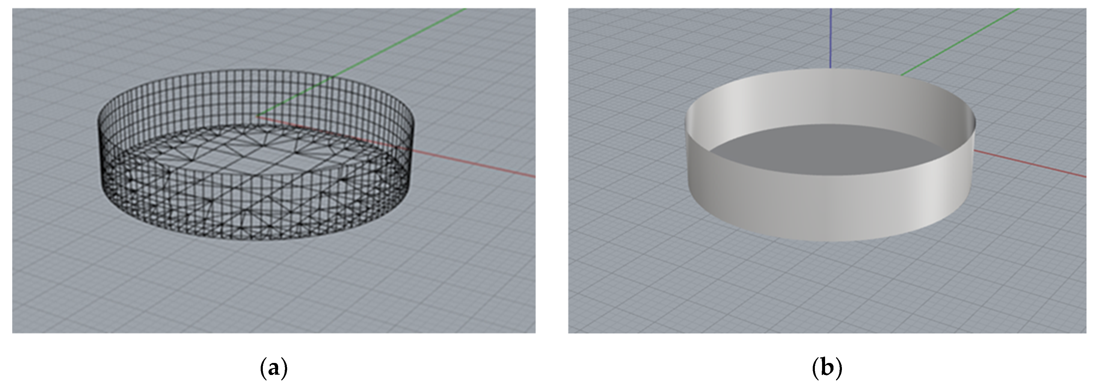
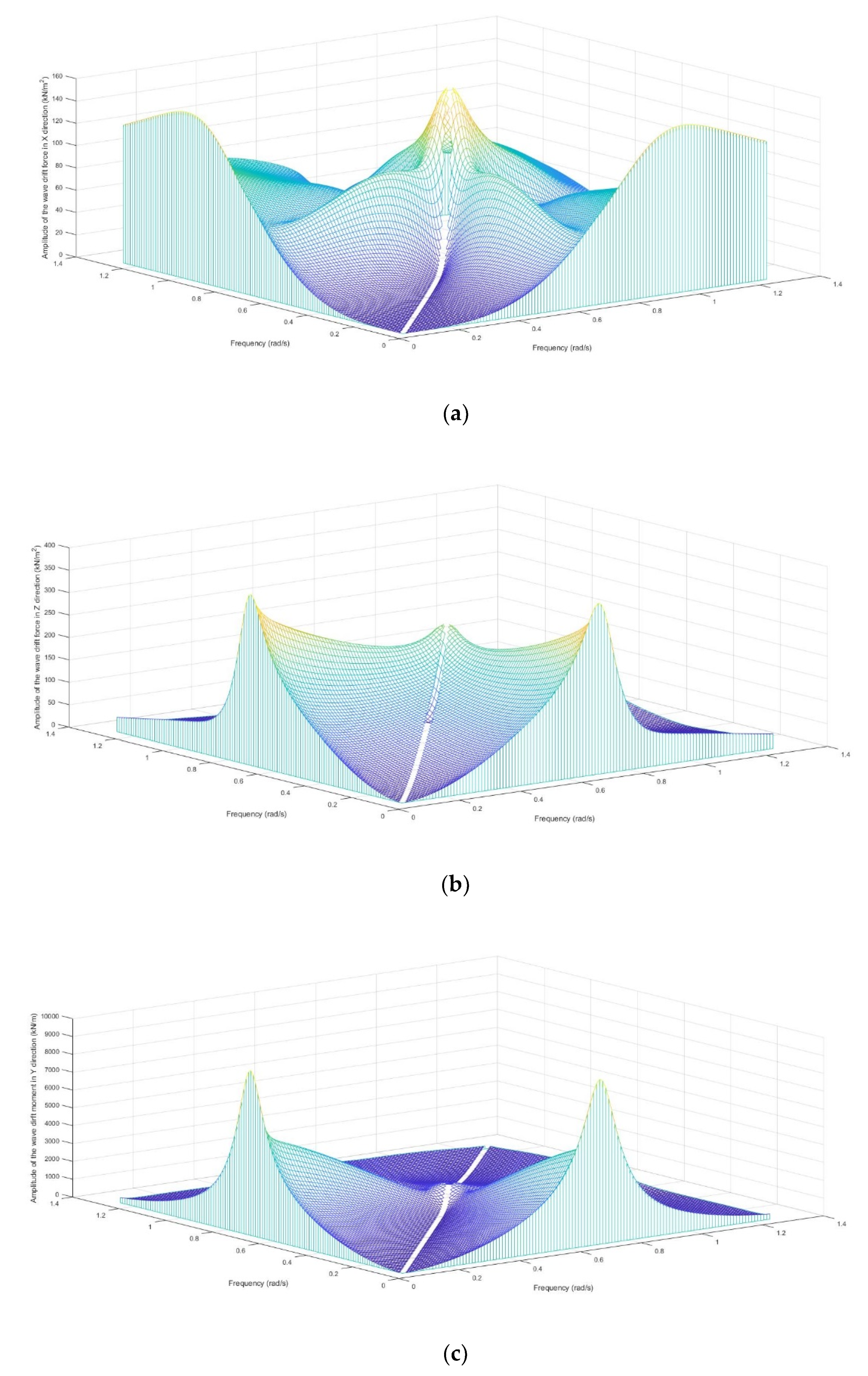
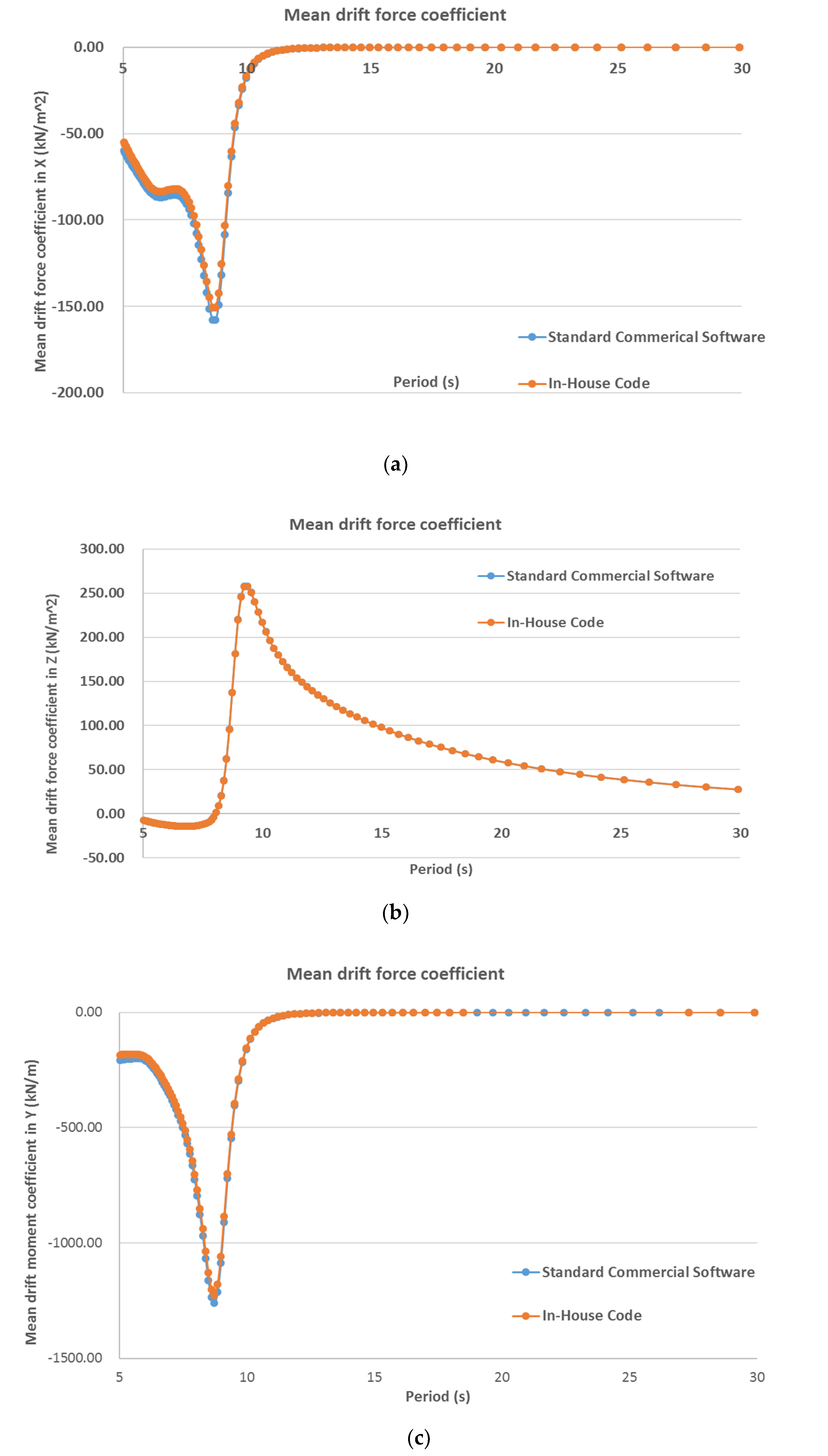
To verify this approach through the direct pressure integral method, a vertical cylinder has been selected as an example. The diameter of the vertical cylinder is 40 m and its draft is 10 m. The center of the gravity is 5 m above the equilibrium free surface. The numerical model and panelization of the vertical cylinder established by Rhino 3D have been shown in Figure 1. The incident wave direction in this numerical evaluation is 180 deg and the water depth is 1500 m. The full quadratic transfer function of the second-order wave loads were numerically estimated through our in-house code and have been presented in Figure 2. The mean drift force coefficients, namely the diagonal elements of the full quadratic function, have been presented and compared with the numerical results from the industry standard commercial software WAMIT as a reference [27] but that code is limited to zero speed. It can be seen from Figure 3 that our in-house code shows a good agreement with the standard commercial software and provides a convincing numerical calculation basis of our approach to calculate the second-order wave loads with zero forward speed.
3. The Neumann-Kelvin and Double-Body Linearization
A well-known linearization scheme in ship hydrodynamics is the Neumann-Kelvin linearization with respect to the forward speed U, whose assumption is that the radiation potential caused by the floating body is less significant than the uniform flow [23]. Moreover, the Kelvin ship waves effects on the free surface and the impact on the flow potential due to the floating body’s shape are negligible, which simplifies the boundary conditions. Therefore, it is also called uniform-flow linearization and applicable for a slender floating body, whose total potential can be expressed as:
where:
In this scenario, denotes the wave potential, ηi denotes the vessel’s motions in 6 degrees of freedom, denotes the wave frequency while is the encounter frequency. denotes the radiation wave potential, and is the wave direction with respect to the vessel-fixed coordinate.
The double-body flow linearization was introduced by Dawson [28], who considers both the forward speed U and the shape of the ship hull. The steady potential on the hull through the Double-Body is calculated by assuming the symmetry of the ship hull with respect to the free surface at z = 0 [23]. In the previous research, the numerically estimated added resistances through these two methodologies show discrepancies, due to the radiation components from different body-boundary conditions.
The total potential:
where Φ is the steady base flow that is of O(1) and is the perturbation potential, which is of O(ε).
The linearized boundary condition for the perturbation potential in the Neumann-Kelvin linearization can be expressed as:
The linearized boundary condition for the perturbation potential in double-body flow linearization can be expressed as:
where = (U − )i + (V + )j, where U and V are the vessel’s forward and lateral speed, respectively; is the vessel’s yaw’s angular speed; is the wave elevation on the free surface. is the m-term containing the interaction between the steady and unsteady solutions. In Neumann-Kelvin linearization with only forward speed U for example: (m1, m2, m3, m4, m5, m6) = (0, 0, 0, 0, Un3, −Un2); with only lateral speed V for example: (m1, m2, m3, m4, m5, m6) = (0, 0, 0, −Vn3, 0, Vn1). On the other hand, in the double-body flow linearization, the m-terms can be expressed as:
More details of the corresponding our forward speed derivations can be found in Appendix B.
4. The 3D Maneuvering Mathematical Model
The mathematical model of the maneuvering motions of ships is now well established. Linear equations of motions will be considered in this scenario, in motion modes of surge, sway, and yaw, while the motions of roll, pitch, and heave are often neglected and not considered in such analysis. Eulerian or vessel fixed coordinate systems with axes at the mid-point of the vessel hull can be applied to describe the ship motions. The hydrodynamic forces and the modes of vessel motions can be expressed as:
where u and v are the longitudinal and lateral velocities and r is the yaw rate. Iz is the moment of inertia with respect to the vertical axis going through the midship point, therefore the horizontal distance between the center of gravity and the midship point is xG. The above hydrodynamics forces and moments acting on the ship can be developed through perturbations, where the hydrodynamic loads are proportional to the perturbation quantities. Xdrift stands for the longitudinal wave drift loads in the seakeeping problem.
Combing the above sets of equations sets with only the linear terms, the linearized equations of maneuvering ship’s motion can be expressed as follows.
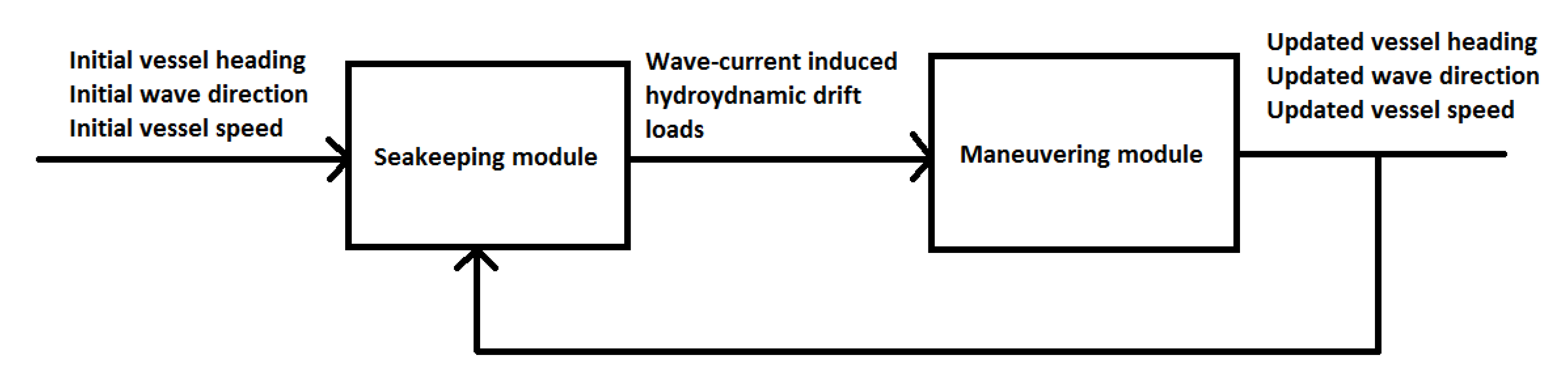
While numerically evaluating a maneuvering ship in waves, there are two modules, namely the seakeeping module and the maneuvering module in each time step, which take the current environmental parameters such as the vessel speed, vessel heading, and wave direction as the input and output the updated input for the next time step. The numerically evaluated hydrodynamic coefficients including the vessel hull, rudder induced loads and the drift loads considering the wave drift damping are all considered as the internal parameters in these two modules. The flow chart of the coupling effect of the seakeeping and maneuvering analysis in terms of slowly varying mean second wave loads that also change the ship speed and wave heading is be presented in Figure 4.
5. Simulation of Maneuvering in Waves
In this study, two vessels were selected, a KVLCC model and KCS model. For the KVLCC model: the Lpp is 320 m, the draught is 20.8 m, and the displacement is 312,622 m3. Four regular waves have been selected, whose ratios of the wave length and the vessel length are 1.25, 1, 0.75 and 0.5, respectively. The vessel’s starting speed is 9.3 knots. Both the turning circle trajectory and zig-zag test time series were numerically evaluated. For the KCS model: the Lpp is 230 m; the draught is 10.8 m; the displacement is 52,030 m3. The experimental maneuvering results carried out by Hiroshima University [29] were chosen as the reference for the turning circle trajectory in both the calm water and regular wave with wave direction of 180 degrees, whose wave length is equal to the vessel length. The vessel’s starting speed in both the calm water and wave tests is Fn = 0.16 (corresponding to a full scale 14.5 knots). In the wave test, the regular wave’s height is 3.61 m in the full scale with a full scale wave period of 12.14 s.
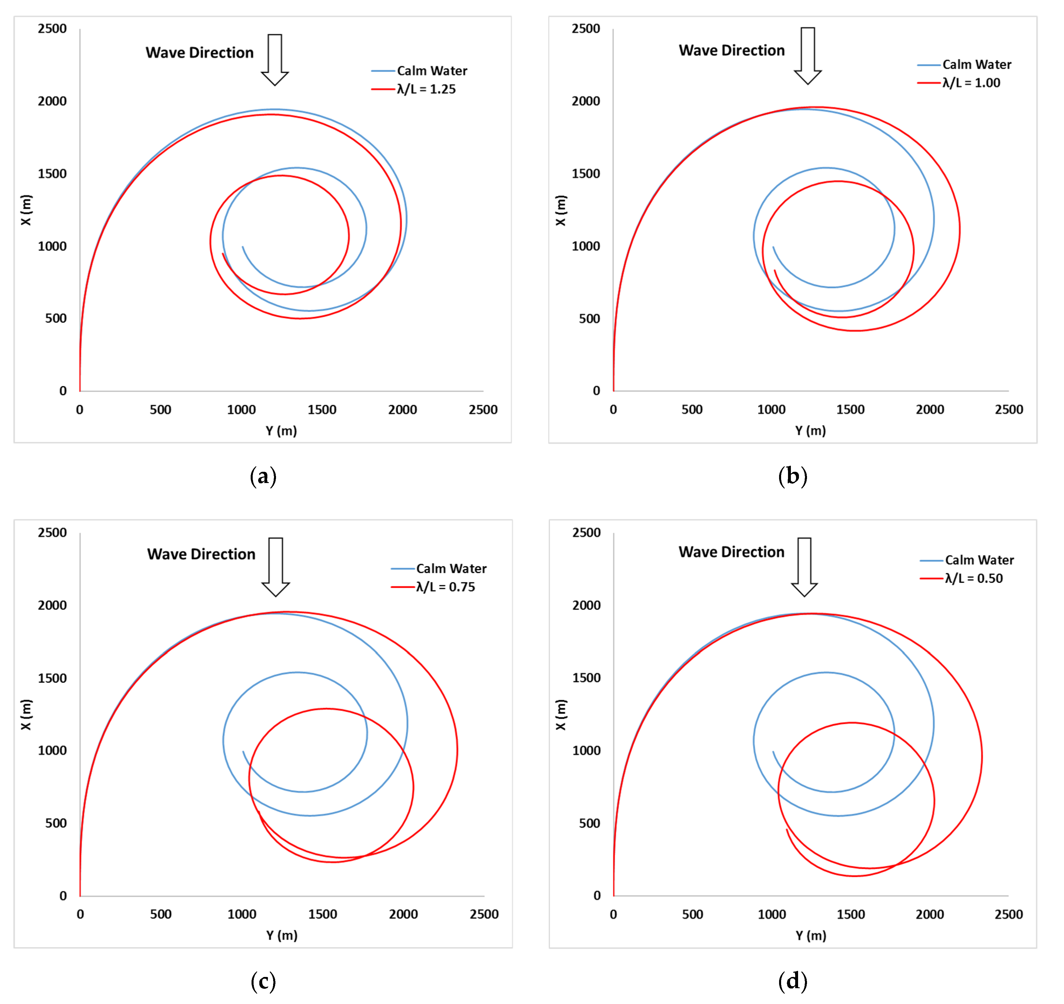
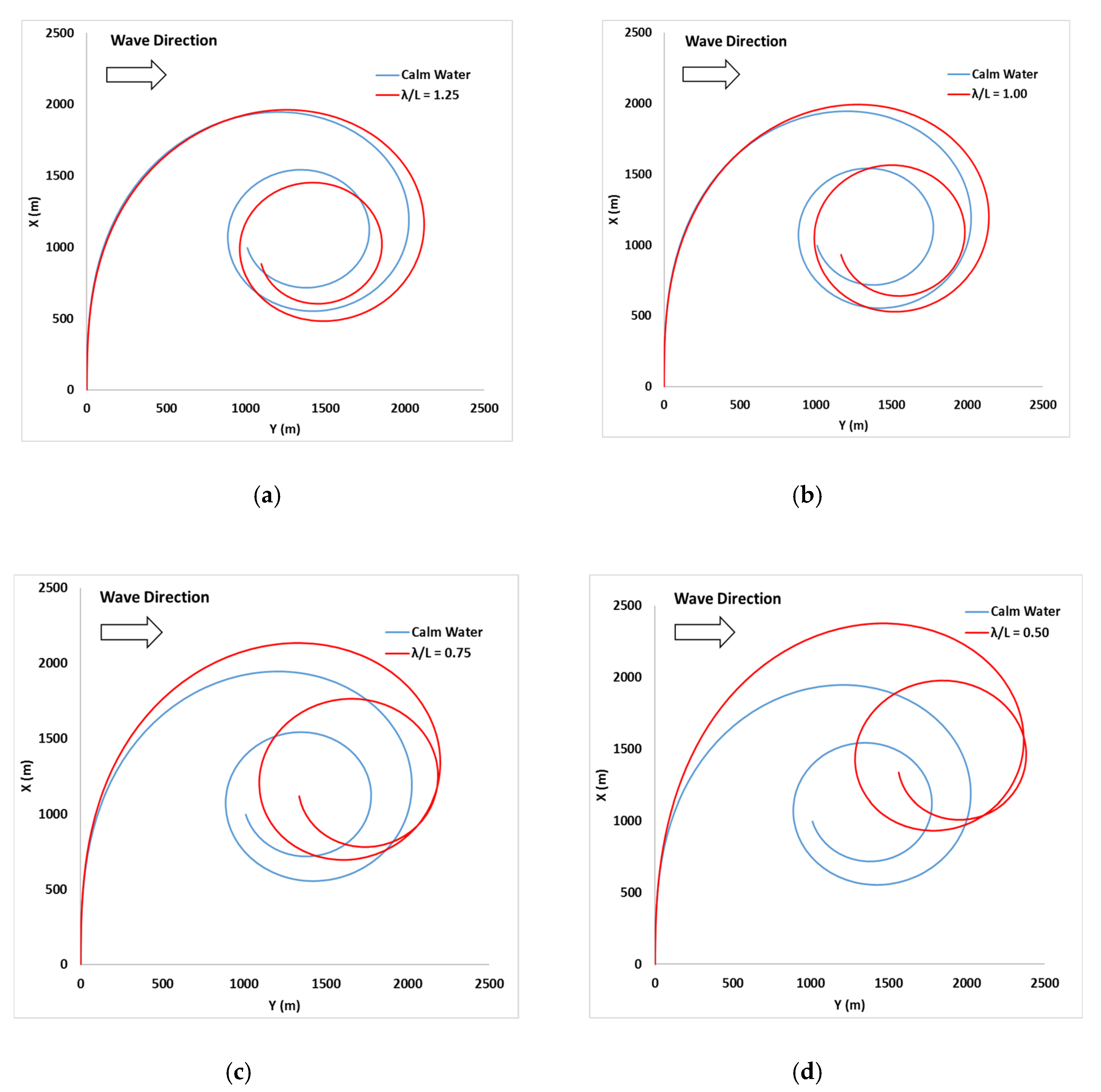
Figure 5 and Figure 6 present the KVLCC’s turning trajectories in regular waves with starboard rudder of 35 degrees. In calm water, the turning trajectory will converge to a stable circle after continuous turning. Compared with the turning trajectories in the calm water, the wave drift loads coupled with wave drift damping drives the vessel turning trajectories to present a horizontal shift path, instead of the stable converged circle. It can be seen that as the wave length decreases, this drifting path is more obvious.
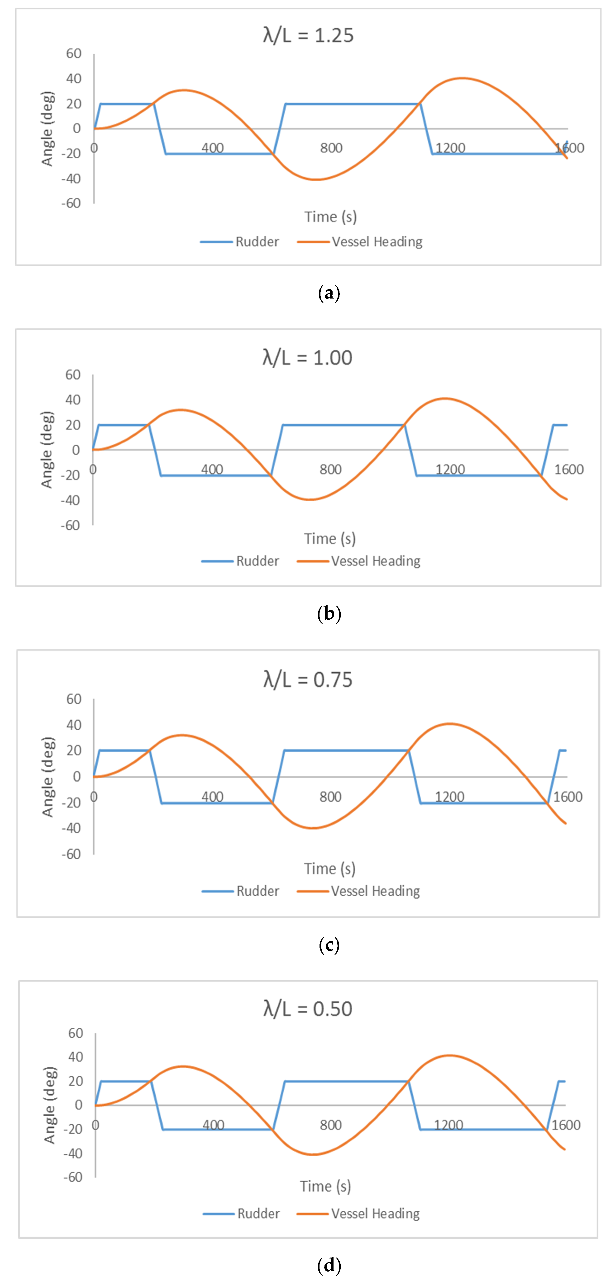
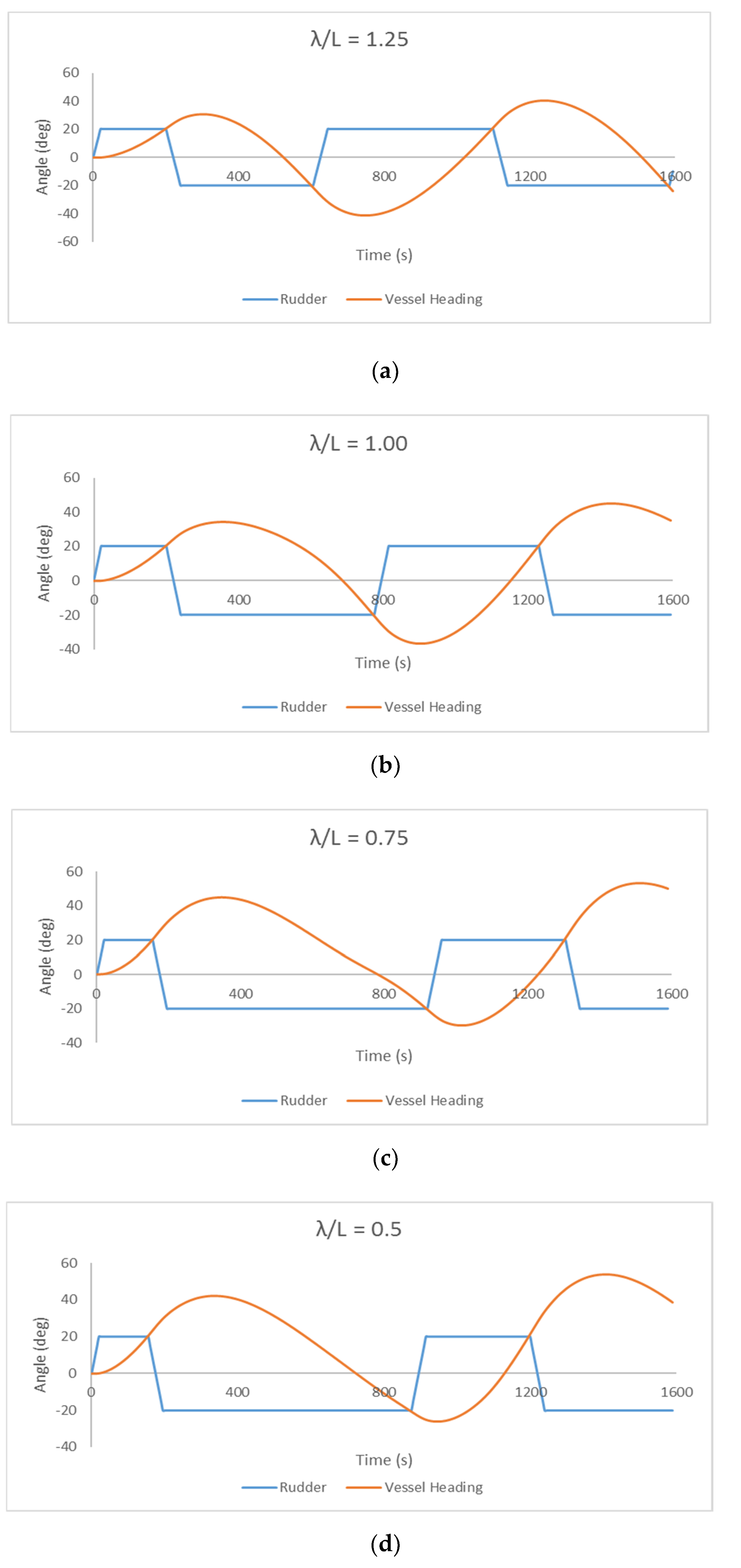
Figure 7 and Figure 8 present the 20/20 deg zig-zag turning test in regular waves with various wave lengths. Compared with the cases in heading sea at the beginning point where the vessel heading presents symmetry characteristic about positive and negative headings, the vessel heading in the cases of beam sea at the starting point presents asymmetric characteristic. In Figure 7, it can be observed that the period of the rudder angle fixed at the 20 deg presents an increasing trend with the zig-zag round. When the wave length is equal to the vessel length in Figure 7b, the vessel turning rate is higher than the cases with other wave lengths. In Figure 8, as the wave length decreases in beam sea, the period of the fixed rudder angle is unbalanced about the positive and negative sides, presenting an asymmetric characteristic.
As shown in Figure 9, Figure 10, Figure 11, Figure 12 and Figure 13, the numerically simulated turning trajectories for the KCS vessel have been presented and compared with the model test results in both calm water and regular waves.
In calm water, as can be seen in Figure 9, the numerically simulated turning trajectory shows an excellent match with the experimental results, providing a convincing comparison basis: the diameter of the turning circle through the numerical simulation is 397.3 m, only 8.64% higher than that of the model test, which is 365.7 m.
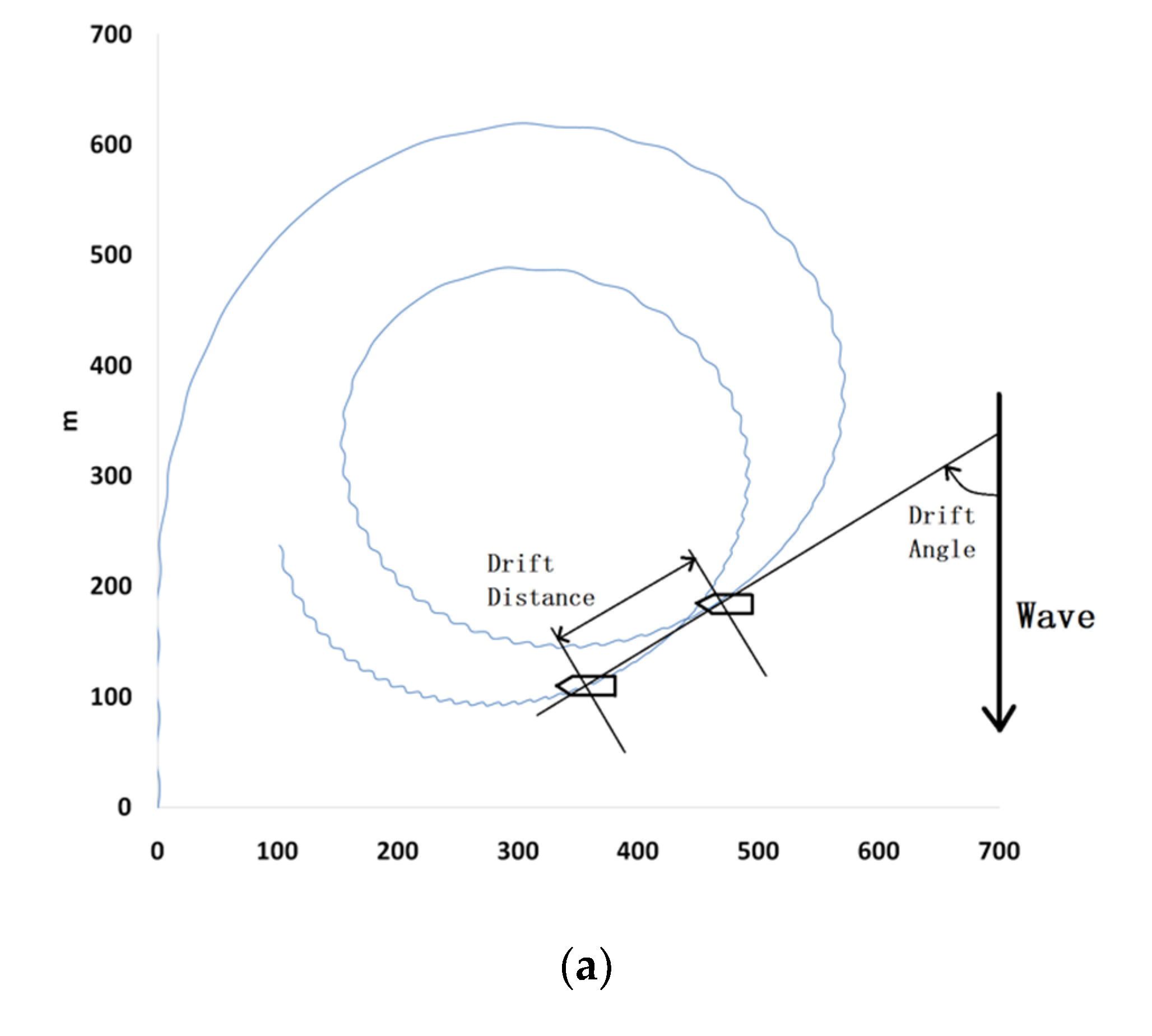
To precisely describe the turning trajectories in waves, multiple parameters including the diameter, the drift angle and the drift distance have been selected in present study. The drift angle is defined as the angle between wave propagating direction and vessel traveling direction in which the wave encounter angle is −90 deg, while the drift distance is defined by successive positions with a wave encounter angle of −90 deg [2]. Two measures of diameter have been considered, namely the diameter measured along with the wave direction (V1 and V2) and the diameter measured perpendicular to the wave direction (H1, H2). These parameters are illustrated in Figure 10.
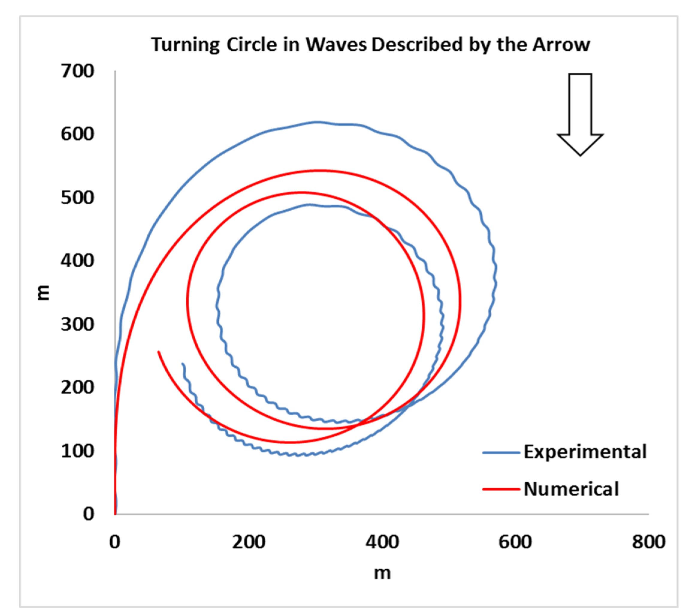
In Figure 11, Figure 12 and Figure 13, a turning trajectory that presents a horizontal shift path due to the waves is observed in the KVLCC model and can also be observed in both the KCS model’s numerical and experimental results. It can be seen in Figure 11 that there is a relatively obvious trajectory shift at the early stage between the numerical and experimental results, which leads to the difference of the corresponding drift angle and drift distance. A similar shift between these two methods can be also found in the calm water results as shown in Figure 9. One reason for this phenomenon is the physical model’s sensitivity to the rudder, which contributes to the discrepancy of the horizontal hydrodynamic loads due to the rudder perturbations, and leads to a shift between the numerical and experimental trajectories. Another reason is the variance of the wake fraction being dependent on the propeller side-wash angle [30], which thus changes the propeller surge force in the model test, while this component was considered as a constant value in the numerical simulation.
Similar discrepancies between the model tests and numerical simulations can also be found in Zhang’s research [7], as well as Lee and Kim’s research [13] through the double-body linearization results with and without a vortex sheet. Also, this is the case in Chillcce and Moctar’s work [14] who applied a RANS computer code to obtain calm water forces and a 3D RANKINE source method to consider the second-order wave forces. It should also be noted that the discrepancies between the numerical and experimental results in most recent research also increase in the later stage of the turning trajectory. As is the case in the present study, after the early stage of the turning trajectory, the numerical simulation matches well with the experimental data, accurately capturing the main turning trajectory’s drifting path. Moreover, the numerically simulated turning trajectory’s diameters have shown a good match with the model test within a 7% discrepancy as presented in Table 1: the H1, V1, H2, and V2 present −2.47%, 6.94%, 0.65%, and −3.48% discrepancies from the model test, respectively.
Therefore, the current framework of coupling the seakeeping and maneuvering modules provides a practical and accurate numerical methodology through the experimental validation, to predict the unconstrained vessel’s maneuvering in waves. Compared with the most recent research [7,13,14], this framework presents a comparatively accurate prediction of the later stage of the turning trajectory in waves. Moreover, with a thorough physical model and explanation of the second-order wave loads through the potential flow theory, this framework is numerically efficient, especially considering CFD’s current large requirement of computational resources [4,5,6]. In the future research, the sensitivity of the physical model in this framework to various hydrodynamic and wave parameters can be conducted and extended for the design of vessels [26,31].
6. Conclusions
In this paper, a framework that considers the coupled maneuvering and seakeeping problems that involves an accurate prediction of the second-order wave loads of a maneuvering vessel in waves has been introduced and validated. An original and systematic perturbation approach to derive the 2nd-order wave loads without and with a vessel’s forward speed have been presented. Moreover, this approach has been validated for zero speed through a comparison to the industry standard commercial code. With the help of the established framework through the two-time scale method and the Neumann-Kelvin linearization, the numerical simulations of maneuvering vessels in waves have been conducted to obtain the turning trajectories and the zig-zag test time series for the KVLCC and KCS models. According to the numerical simulations, the wave drift loads with wave drift damping drives the vessel turning trajectory away from the calm water trajectory, resulting in a drifting path. As the wave length decreases, this drifting phenomenon is more pronounced. It can also be concluded that maneuvering in beam seas also presents an asymmetric characteristic for the vessel heading in the zig-zag tests. Through the comparison with the KCS model test and other recent approaches, the corresponding numerical result accurately captures the main characteristic of the turning trajectory, especially in the later stage. Therefore, the framework herein is an accurate and efficient approach to study the maneuvering of ships in waves. In future work, the current framework can be extended and contribute to the IMO standards for determining the minimum propulsion power to guarantee the maneuverability of vessels in adverse conditions.
Author Contributions
Conceptualization, Z.X. and J.F.; methodology, Z.X. and J.F.; software, Z.X.; validation, Z.X.; formal analysis, Z.X., J.F., and H.W.; investigation, Z.X. and J.F.; data curation, Z.X.; writing—original draft preparation, Z.X.; writing—review and editing, Z.X., J.F., and H.W.; visualization, Z.X.; supervision, J.F.; funding acquisition, J.F. All authors have read and agreed to the published version of the manuscript.
Funding
This research received no external funding.
Acknowledgments
The authors really appreciate the open-source model test data provided by Hiroshima University.
Conflicts of Interest
The authors declare no conflict of interest.
Nomenclature
| X: global coordinate. |
| X’: vessel-fixed coordinate. |
| X0: the origin of the vessel-fixed coordinate in the global coordinate. |
| S: the exact wetted surface of the floating structure. |
| SM: the equilibrium wet surface of the floating structure. |
| p: wave pressure. |
| Φ denotes the wave potential. |
| ζ denotes the wave elevation on the free water surface. |
| n denotes the normal vector of the panel. |
| ηi denotes the 6 degrees of freedom motions: surge, sway, heave, roll, pitch and yaw. |
| η = (η1, η2, η3)T |
| α = (η4, η5, η6)T |
| U and V are the vessel’s forward and lateral speed, respectively |
| ΩR is the vessel’s yaw speed |
| W = (U − ΩRy)i + (V + ΩRx)j |
Appendix A. Derivation of the 2nd-Oder Wave Loads without Forward Speed
A point fixed on the floating structure’s surface can be studied both in the global coordinate and the vessel-fixed coordinate. Assuming small amplitude of the floating structure’s angular motion, the transformation between the global coordinate and the vessel-fixed coordinate can be approximated as:
Through the perturbation theory, we can determine the wave pressure, the normal vector, the floating structure’s motions, the wave potential and the wave elevation into the form of a summation of different orders:
Through the coordinate transformation, we have:
Therefore, we could obtain:
By applying the Bernoulli equation,
the pressure on the floating structure can be expressed as:
Therefore, by collecting the ε0, ε, and ε2 terms, we could obtain the wave pressure in different orders:
Similarly, the normal vector of the floating structure’s wetted surface pointing into the fluid field can also be expressed in both global and vessel-fixed coordinate:
Therefore, we could obtain:
Then, we obtain the expression of wave load in various orders:
where:
Now, we discuss the term :
The integration of is of order 3 and thus out of consideration in this scenario.
Therefore, we could obtain:
This term will be taken into consideration while evaluating the second-order wave loads. It should be noted that the normal vector in z-direction plays an important role that is also called the flare angle effect [32] determining the whole term’s contribution, where is the normal vector of the waterline panel towards the fluid field. For a wall-sided waterline panel, the amplification of the flare angle effect is 1. However, as the normal vector’s z-direction component increases from 0 to 1, this amplification increases significantly. In such treatment situations, caution should be taken.
According to our previous study on the numerical evaluation of the full quadratic transfer function, the full expression of the second-order wave loads on a floating body can be expressed as:
where:
Appendix B. The 2nd-Order Wave Loads with Forward Speed
The boundary condition has been modified, due to the vessel’s forward speed. The scattered wave potential in this scenario and the Green function should be evaluated in ω0 and ωe, respectively.
Through Greens identity and a variant of Stokes theorem that the forward speed boundary value problem can be solved through obtaining the boundary condition in zero speed and modification [33]. The wave loads from the scattered wave potential can be evaluated.
For normal vectors direction towards the fluid domain, the above equation can be written as:
where:
To evaluate the 1st-order wave forces and moments due to the scattered potential, its expression through direct pressure integration can be written as:
Therefore, while there is an arbitrary basis flow including head seas and quartering seas, F(1)sca in jth mode can be so thus expressed as:
According to Kim and Kim [23], the added resistance due to the forward speed or current in waves is the longitudinal component of the mean drift force, whose expression based on the double-body linearization scheme can be written as:
By substituting Φ as zero, the mean drift force of the Neumann-Kelvin linearization scheme can be obtained.
References
- Nomoto, K.; Taguchi, T.; Honda, K.; Hirano, S. On the steering qualities of ships. Int. Shipbuild. Prog. 1957, 4, 354–370. [Google Scholar] [CrossRef]
- Ueno, M.; Nimura, T.; Miyazaki, H. Experimental study on maneuvering motion of a ship in waves. In Proceedings of the International Conference on Marine Simulation and Ship Maneuverability, Kanazawa, Japan, 25–28 August 2003. [Google Scholar]
- Kim, D.J.; Yun, K.; Park, J.; Yeo, D.J.; Kim, Y.G. Experimental investigation on turning characteristics of KVLCC2 tanker in regular waves. Ocean Eng. 2019, 175, 197–206. [Google Scholar]
- Islam, H.; Soares, C.G. Estimation of hydrodynamic derivatives of a container ship using PMM simulation in OpenFOAM. Ocean Eng. 2018, 164, 414–425. [Google Scholar]
- Uharek, S.; Cura-Hochbaum, A. The influence of inertial effects on the mean forces and moments on a ship sailing in oblique waves Part B: Numerical prediction using a RANS code. Ocean Eng. 2018, 165, 264–276. [Google Scholar]
- Wang, J.H.; Zou, L.; Wan, D.C. Numerical simulations of zigzag maneuver of free running ship in waves by RANS-Overset grid method. Ocean Eng. 2018, 162, 55–79. [Google Scholar]
- Zhang, W.; Zou, Z.J.; Deng, D.P. A study on prediction of ship maneuvering in regular waves. Ocean Eng. 2017, 137, 367–381. [Google Scholar] [CrossRef]
- Skejic, R. Ships maneuvering simulations in a seaway-How close are we to reality? In Proceedings of the International Workshop on Next Generation Nautical Traffic Models, Delft, The Netherlands, July 2013. [Google Scholar]
- Bailey, P.A.; Price, W.G.; Temarel, P. A unified mathematical model describing the maneuvering of a ship travelling in a seaway. Trans. R. Inst. Nav. Archit. 1997, 140, 131–149. [Google Scholar]
- Lee, S.K.; Hwang, S.H.; Yun, S.W.; Rhee, K.P.; Seong, W.J. An experimental study of a ship maneuverability in regular waves. In Proceedings of the International Conference on Marine Simulation and Ship Maneuverability, Panama City, Panama, 17–20 August 2009. [Google Scholar]
- Skejic, R.; Faltinsen, O.M. A unified seakeeping and maneuvering analysis of ships in regular waves. J. Mar. Sci. Technol. 2008, 13, 371–394. [Google Scholar] [CrossRef]
- Seo, M.G.; Kim, Y. Numerical analysis on ship maneuvering coupled with ship motion in waves. Ocean Eng. 2011, 38, 1934–1945. [Google Scholar] [CrossRef]
- Lee, J.; Kim, Y. Study on steady flow approximation in turning simulation of ship in waves. Ocean Eng. 2020, 195, 106645. [Google Scholar] [CrossRef]
- Chillcce, G.; Moctar, O. A numerical method for maneuvering simulation in regular waves. Ocean Eng. 2018, 170, 434–444. [Google Scholar] [CrossRef]
- Xie, Z.T.; Liu, Y.J.; Falzarano, J. A numerical evaluation of the quadratic transfer function for a floating structure. In Proceedings of the ASME 2019 38th International Conference on Ocean, Offshore and Arctic Engineering, Glasgow, Scotland, UK, 9–14 June 2019. [Google Scholar]
- Newman, J.N. Second-order slowly varying forces of vessels in irregular waves. In Proceedings of the International Symposium on Dynamics of Marine Vehicles and Structures in Waves, IMechE, London, UK, 4 January 1974. [Google Scholar]
- Aranha, J.A.P. A formula for ‘wave damping’ in the drift of a floating body. J. Fluid Mech. 1994, 275, 147–155. [Google Scholar] [CrossRef]
- Aranha, J.A.P. Second-order horizontal steady forces and moment on a floating body with small forward speed. J. Fluid Mech. 1996, 313, 39–54. [Google Scholar] [CrossRef]
- Aranha, J.A.P.; Fernandes, A.C. On the second-order slow drift force spectrum. Appl. Ocean Res. 1995, 17, 311–313. [Google Scholar] [CrossRef]
- Aranha, J.A.P.; da Silva, S.; Martins, M.R.; Leite, A.J.P. A weathervane ship under wave and current action: An experimental verification of the wave drift damping formula. Appl. Ocean Res. 2001, 23, 103–110. [Google Scholar] [CrossRef]
- Trassoudaine, D.; Naciri, M. A comparison of a heuristic wave drift damping formula with experimental Results. Appl. Ocean Res. 1999, 21, 93–97. [Google Scholar] [CrossRef]
- Joncquez, S.A.G. Second-order forces and moments acting on ships in waves. PhD Thesis, Technical University of Denmark, Copenhagen, Denmark, 2009. [Google Scholar]
- Kim, K.H.; Kim, Y.H. Comparative study on ship hydrodynamics based on neumann-kelvin and double-body linearization in time-domain analysis. Int. J. Offshore Polar Eng. 2010, 20, 265–274. [Google Scholar]
- Yu, M.; Falzarano, J. A comparison of the neumann-kelvin and rankine source methods for wave resistance calculations. Ocean Syst. Eng. 2017, 7, 371–398. [Google Scholar]
- Xie, Z.T.; Falzarano, J. Study on 2nd-order wave loads with forward speed through aranha’s formula and neumann-kelvin linearization. In Proceedings of the ASME 2020 39th International Conference on Ocean, Offshore and Arctic Engineering, Fort Lauderdale, FL, USA, 28 June–3 July 2020. [Google Scholar]
- 2013 Interim Guidelines for Determining Minimum Propulsion Power to Maintain the Maneuverability of Ships in Adverse Conditions, as Amended (Resolution MEPC.232(65), as Amended by Resolutions MEPC.255(67) and MEPC.262(68)); International Maritime Organization: London, UK, 15 July 2015.
- WAMIT Software. In WAMIT User Manual; WAMIT Inc.: Chestnut Hill, MA, USA.
- Dawson, C.W. A practical computer method for solving ship-wave problem. In Proceedings of the Second International Conference on Numerical Ship Hydrodynamics, Berkeley, CA, USA, 1 January 1977. [Google Scholar]
- Available online: http://www.simman2019.kr/contents/KCS.php (accessed on 20 March 2020).
- Sutulo, S.; Soares, C.G. On the application of empriric methods for prediction of ship maneuvering properties and associated uncertainties. Ocean Eng. 2019, 186, 106111. [Google Scholar] [CrossRef]
- Hirdaris, S.E.; Bai, W.; Dessi, D.; Ergin, A.; Gu, X.; Hermundstad, O.A.; Huijsmans, R.; Iijima, K.; Nielsen, U.D.; Parunov, J.; et al. Loads for use in the design of ships and offshore structures. Ocean Eng. 2014, 78, 131–174. [Google Scholar] [CrossRef]
- Guha, A.; Falzarano, J. The effect of hull emergence angle on the near field formulation of added resistance. Ocean Eng. 2015, 105, 10–24. [Google Scholar] [CrossRef]
- Guha, A.; Falzarano, J. Estimation of hydrodynamic forces and motions of ships with steady forward speed. Int. Shipbuild. Prog. 2015, 62, 113–138. [Google Scholar] [CrossRef]
Figure 1.
The numerical model of the vertical cylinder: (a) Description of the vertical cylinder; (b) Numerical panel of the vertical cylinder.
Figure 1.
The numerical model of the vertical cylinder: (a) Description of the vertical cylinder; (b) Numerical panel of the vertical cylinder.

Figure 2.
The amplitudes of the drift force coefficients with respect to wave frequencies (rad/s): (a) Amplitude of the wave drift force in X direction (kN/m2); (b) Amplitude of the wave drift force in Z direction (kN/m2); (c) Amplitude of the wave drift moment in Y direction (kN/m).
Figure 2.
The amplitudes of the drift force coefficients with respect to wave frequencies (rad/s): (a) Amplitude of the wave drift force in X direction (kN/m2); (b) Amplitude of the wave drift force in Z direction (kN/m2); (c) Amplitude of the wave drift moment in Y direction (kN/m).

Figure 3.
The comparison of the mean drift force coefficients with the standard commercial software: (a) Amplitude of the mean drift force in X direction (kN/m2); (b) Amplitude of the mean drift force in Z direction (kN/m2); (c) Amplitude of the mean drift moment in Y direction (kN/m).
Figure 3.
The comparison of the mean drift force coefficients with the standard commercial software: (a) Amplitude of the mean drift force in X direction (kN/m2); (b) Amplitude of the mean drift force in Z direction (kN/m2); (c) Amplitude of the mean drift moment in Y direction (kN/m).

Figure 4.
Process diagram of numerical maneuvering model.

Figure 5.
KVLCC’s starboard-side 35 deg turning trajectories in regular waves with 180 deg at t = 0 and four different ratios between wave length and vessel length λ: (a) λ = 1.25; (b) λ = 1; (c) λ = 0.75; (d) λ = 0.5.
Figure 5.
KVLCC’s starboard-side 35 deg turning trajectories in regular waves with 180 deg at t = 0 and four different ratios between wave length and vessel length λ: (a) λ = 1.25; (b) λ = 1; (c) λ = 0.75; (d) λ = 0.5.

Figure 6.
KVLCC’s starboard-side 35 deg turning trajectories in regular waves with 90 deg at t = 0 and four different ratios between wave length and vessel length λ: (a) λ = 1.25; (b) λ = 1; (c) λ = 0.75; (d) λ = 0.5.
Figure 6.
KVLCC’s starboard-side 35 deg turning trajectories in regular waves with 90 deg at t = 0 and four different ratios between wave length and vessel length λ: (a) λ = 1.25; (b) λ = 1; (c) λ = 0.75; (d) λ = 0.5.

Figure 7.
KVLCC’s 20/20 (starboard-side) Zig-Zag tests in regular waves with 180 deg at t = 0 and four different ratios between wave length and vessel length λ: (a) λ = 1.25; (b) λ = 1; (c) λ = 0.75; (d) λ = 0.5.
Figure 7.
KVLCC’s 20/20 (starboard-side) Zig-Zag tests in regular waves with 180 deg at t = 0 and four different ratios between wave length and vessel length λ: (a) λ = 1.25; (b) λ = 1; (c) λ = 0.75; (d) λ = 0.5.

Figure 8.
KVLCC’s 20/20 (starboard-side) Zig-Zag tests in regular waves with 90 deg at t = 0 and four different ratios between wave length and vessel length λ: (a) λ = 1.25; (b) λ = 1; (c) λ = 0.75; (d) λ = 0.5.
Figure 8.
KVLCC’s 20/20 (starboard-side) Zig-Zag tests in regular waves with 90 deg at t = 0 and four different ratios between wave length and vessel length λ: (a) λ = 1.25; (b) λ = 1; (c) λ = 0.75; (d) λ = 0.5.

Figure 9.
KCS’s experimental and numerical starboard-side 35 deg turning trajectories in calm water.
Figure 9.
KCS’s experimental and numerical starboard-side 35 deg turning trajectories in calm water.

Figure 10.
Parameters of the turning trajectory in waves: (a) Drift angle and drift distance; (b) Horizontal and vertical diameter of the turning trajectory.
Figure 10.
Parameters of the turning trajectory in waves: (a) Drift angle and drift distance; (b) Horizontal and vertical diameter of the turning trajectory.


Figure 11.
KCS’s experimental and numerical starboard-side 35 deg turning trajectories regular wave with 180 deg at t = 0.
Figure 11.
KCS’s experimental and numerical starboard-side 35 deg turning trajectories regular wave with 180 deg at t = 0.

Figure 12.
KCS’s experimental starboard-side 35 deg turning trajectories in calm water and regular wave with 180 deg at t = 0.
Figure 12.
KCS’s experimental starboard-side 35 deg turning trajectories in calm water and regular wave with 180 deg at t = 0.

Figure 13.
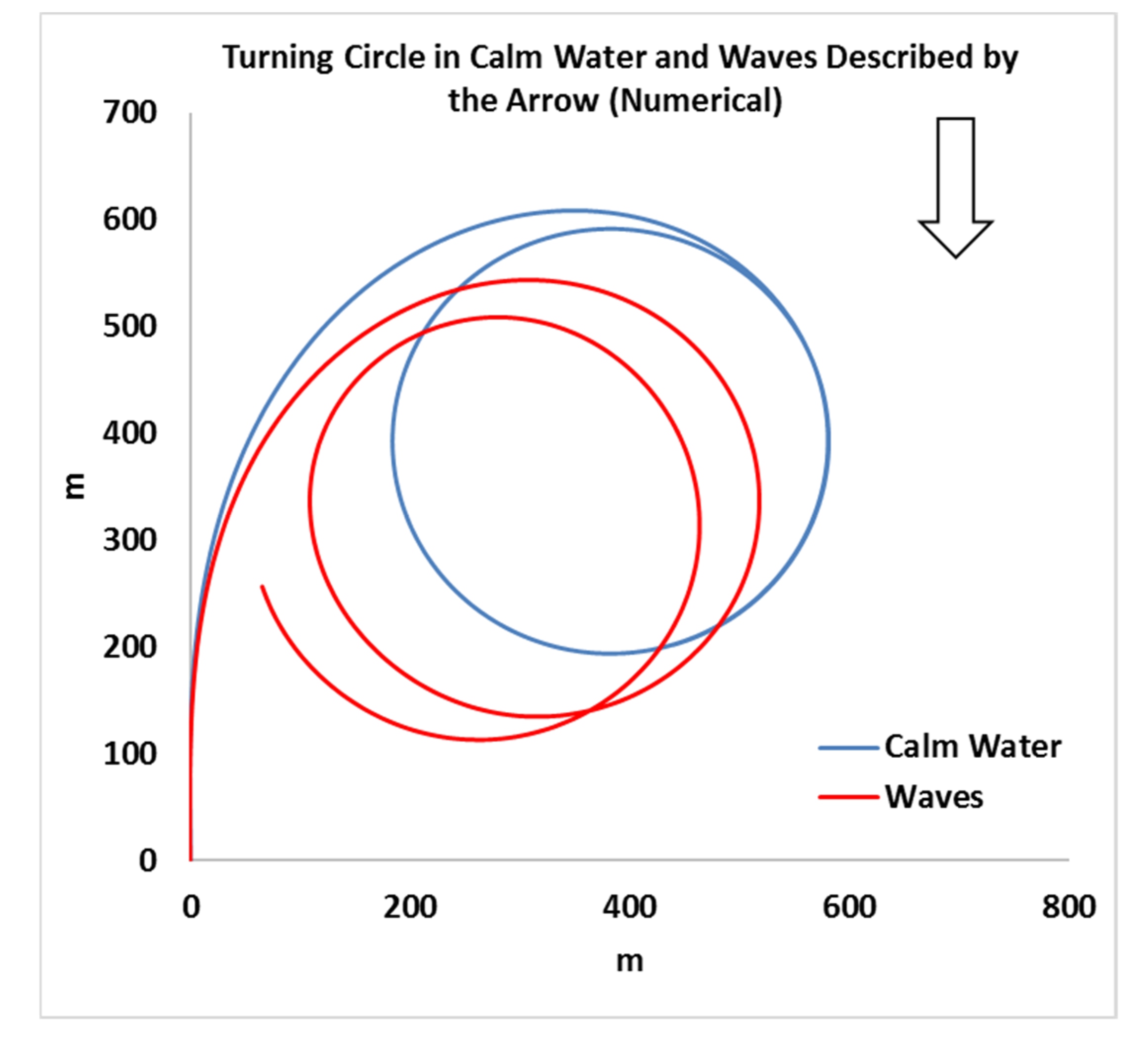
KCS’s numerical starboard-side 35 deg turning trajectories in calm water and regular wave with 180 deg at t = 0.
Figure 13.
KCS’s numerical starboard-side 35 deg turning trajectories in calm water and regular wave with 180 deg at t = 0.


Table 1.
Parameters of the turning trajectories in calm water and waves.
| D | H1 | V1 | H2 | V2 | Drift Angle | Drift Distance | |
|---|---|---|---|---|---|---|---|
| Unit | m | m | m | m | m | deg | m |
| Model test | 365.7 | 339.8 | 344.3 | 396.1 | 396.5 | 51.9 | 82.6 |
| Numerical simulation | 397.3 | 331.4 | 368.2 | 393.5 | 382.7 | 65.6 | 72.5 |
© 2020 by the authors. Licensee MDPI, Basel, Switzerland. This article is an open access article distributed under the terms and conditions of the Creative Commons Attribution (CC BY) license (http://creativecommons.org/licenses/by/4.0/).
Share and Cite
MDPI and ACS Style
Xie, Z.; Falzarano, J.; Wang, H. A Framework of Numerically Evaluating a Maneuvering Vessel in Waves. J. Mar. Sci. Eng. 2020, 8, 392. https://doi.org/10.3390/jmse8060392
AMA Style
Xie Z, Falzarano J, Wang H. A Framework of Numerically Evaluating a Maneuvering Vessel in Waves. Journal of Marine Science and Engineering. 2020; 8(6):392. https://doi.org/10.3390/jmse8060392
Chicago/Turabian StyleXie, Zhitian, Jeffrey Falzarano, and Hao Wang. 2020. "A Framework of Numerically Evaluating a Maneuvering Vessel in Waves" Journal of Marine Science and Engineering 8, no. 6: 392. https://doi.org/10.3390/jmse8060392
Note that from the first issue of 2016, this journal uses article numbers instead of page numbers. See further details here.