Unsteady RANS CFD Simulations of Sailboat’s Hull and Comparison with Full-Scale Test

Abstract

The hydrodynamic investigation of a hull’s performance is a key aspect when designing a new prototype, especially when it comes to a competitive/racing environment. This paper purports to perform a fully nonlinear unsteady Reynolds Averaged Navier-Stokes (RANS) simulation to predict the motion and hydrodynamic resistance of a sailboat, thus creating a reliable tool for designing a new hull or refining the design of an existing one. A comprehensive range of speeds is explored, and results are validated with hydrodynamic full-scale tests, conducted in the towing tank facility at University of Naples Federico II, Italy. In particular, this work deals with numerical ventilation, which is a typical issue occurring when modeling a hull; a simple and effective solution is here proposed and investigated, based on the phase-interaction substitution procedure. Results of the computational fluid dynamic (CFD) campaign agree with the experimental fluid dynamic (EFD) within a 2% margin.

1. Introduction

The design of a new sailboat prototype is complex and requires time, experience, and resources. It is important to draw several hull shapes and understand which behaves better at sea, as well as to consider the complexity of the boat system and meteorological conditions.

Experience and computer-aided design (CAD) software help the engineer to explore several promising concepts and forms; however, quantitative evaluation of the performance requires tests, either numerical or physical, by means of towing tank tests (TTTs) [1].

The hydrodynamic testing of a new hull is a mandatory step, requiring considerable resources, in terms of time and economic capital, since different prototype models must be built and tested in the tank [2]. Tests can take up to weeks or even months considering all phases involved, from transportation, setup, and calibration, to the actual test and post-processing.

Moreover, most of the time, it is not possible to simulate the real-scale experiment because the cost of realizing a full-scale model is usually prohibitive and, most importantly, towing tanks have limitations for the maximum beam, length, and velocity that can be tested in order to avoid blockage effects and wave reflection [3]. This means that once the analysis is completed, results must be scaled, potentially introducing errors [4].

On the other hand, in the last decades, numerical tanks have become quite popular: The main reason is the cheap availability of computational power, which is now accessible to many designers, researchers, and even students. The widespread use of computational fluid dynamics (CFD) for naval and marine application [5] has also provided the community of users with a set of best practices and state-of-the-art modeling techniques [6,7], which allow the engineers to obtain better results from their CFD towing tank (CTT) and reduce the need for real test validation [8].

At the current stage of development, CFD cannot entirely replace real tests, which are still necessary when realizing a new boat; however, based on the several advantages of CFD over physical experiments and an increasing confidence in CFD setup and results [9,10], numerical simulation will tend to supplant real tests. A fast, cheap, and high-fidelity method, CFD is now used in almost every study of the hydrodynamics of sailboats, or ships in general [11].

An important advantage of numerical tests is flexibility, which makes it possible to easily change the model characteristics (e.g., shape, wetted surface, trim angle, fixed and moving mass distribution), which is crucial at the design stage.

This paper deals with the definition of a CFD setup for a numerical towing tank test and the comparison of the model with a full-scale experimental test. Moreover, a case with numerical ventilation, which is likely to occur when simulating a hull [7,12,13], even for low speeds, is analyzed and two different techniques to solve the problem are presented.

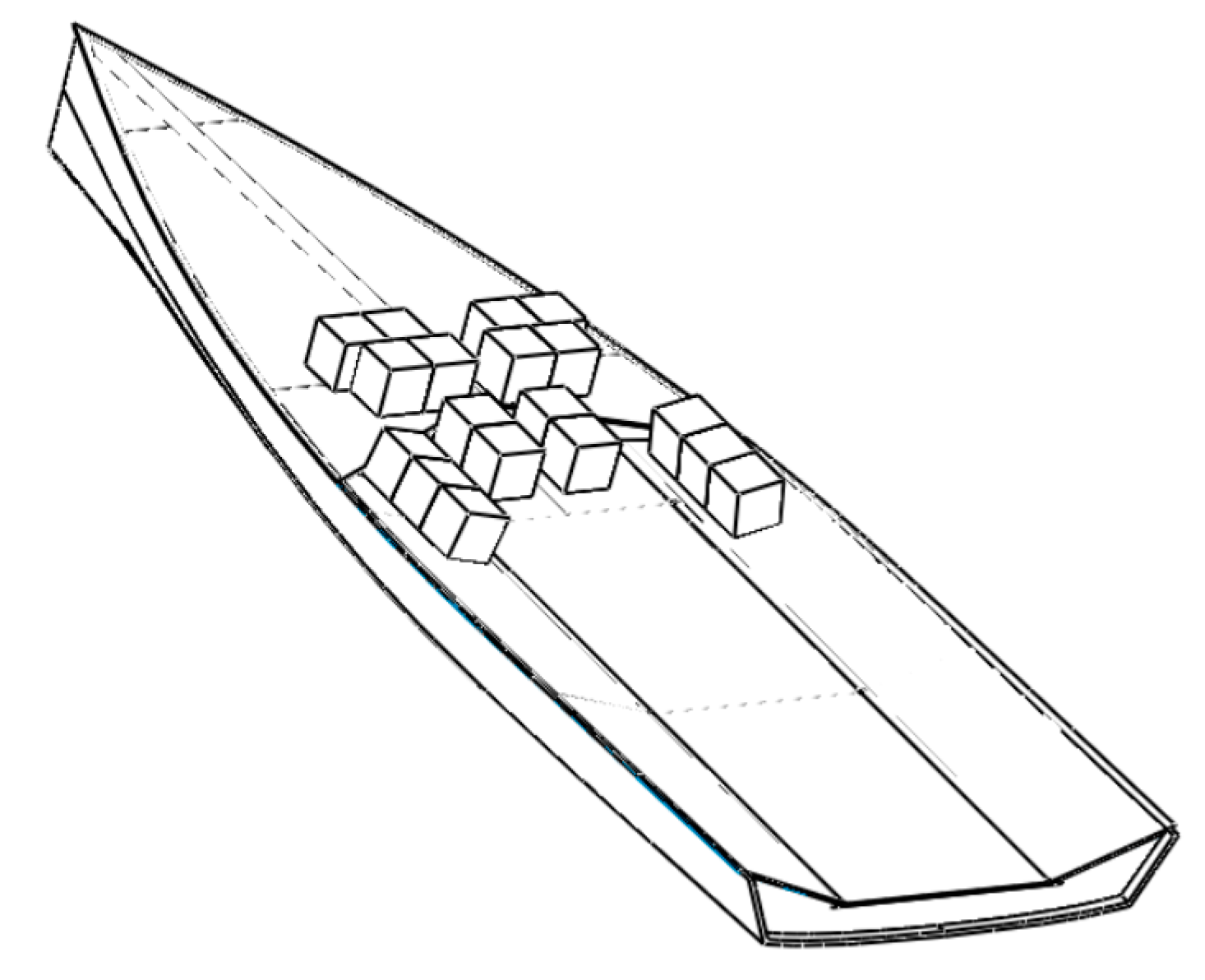
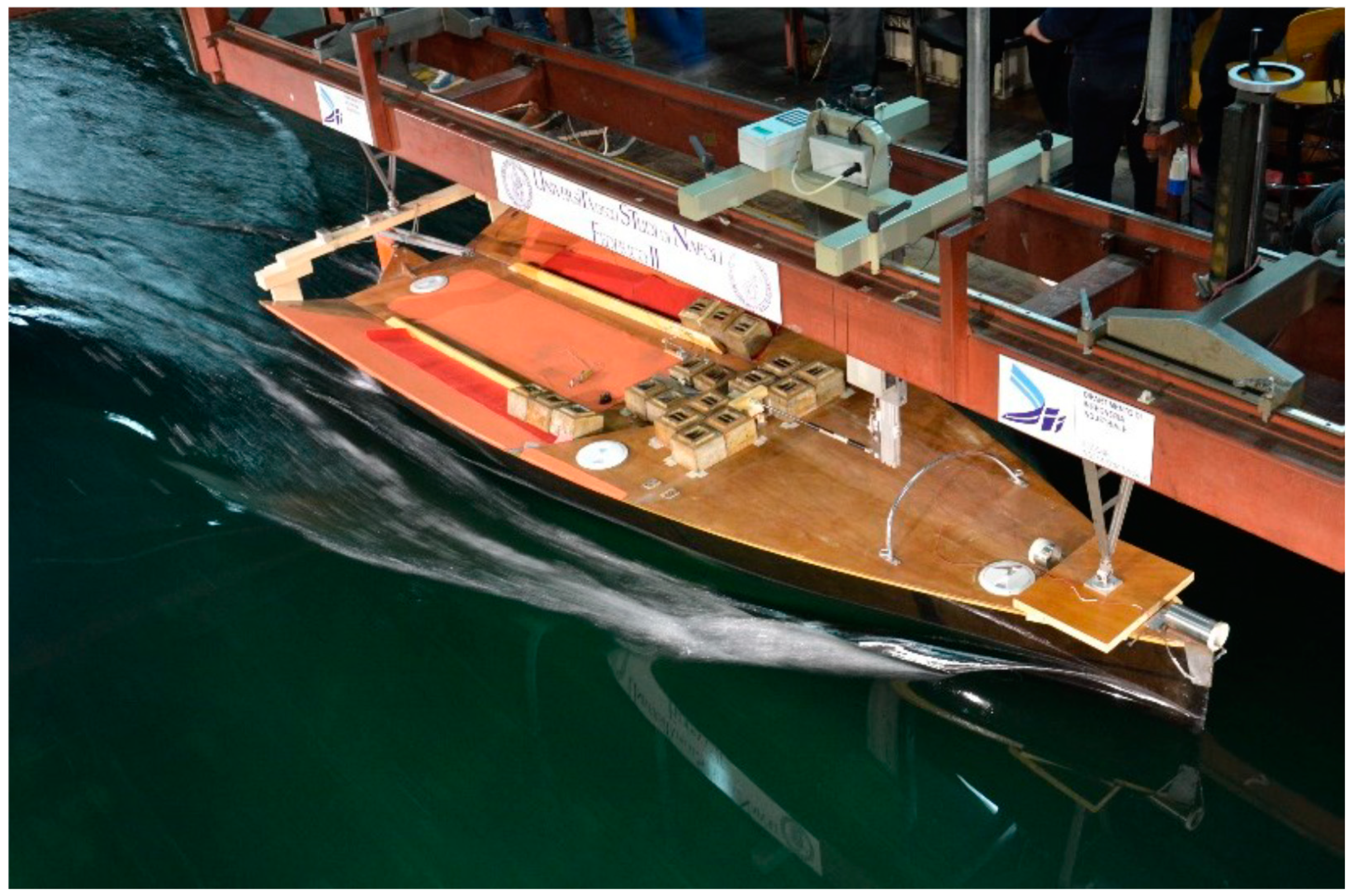
The scope of this numerical and experimental campaign is to mimic real tank tests and to evaluate the drag and the best trim angle for the hull in order to optimize the distribution of the moving weight on board. To gain a greater insight into the non-linear behavior of the hull, three different speeds were tested: 1, 2, and 3 m/s, which correspond respectively to a Froude number of 0.1488, 0.2977, and 0.4465, since the length of water line (LWL) does not change over the three speeds tested and is equal to 4.60 m.

The first two velocities correspond to a displacing mode, the latter to a semi-planing asset.

The towing tank test was carried out at University of Naples Federico II during the Midwinter Indoor Race, a spin-off from the 1001Vela Cup competition.

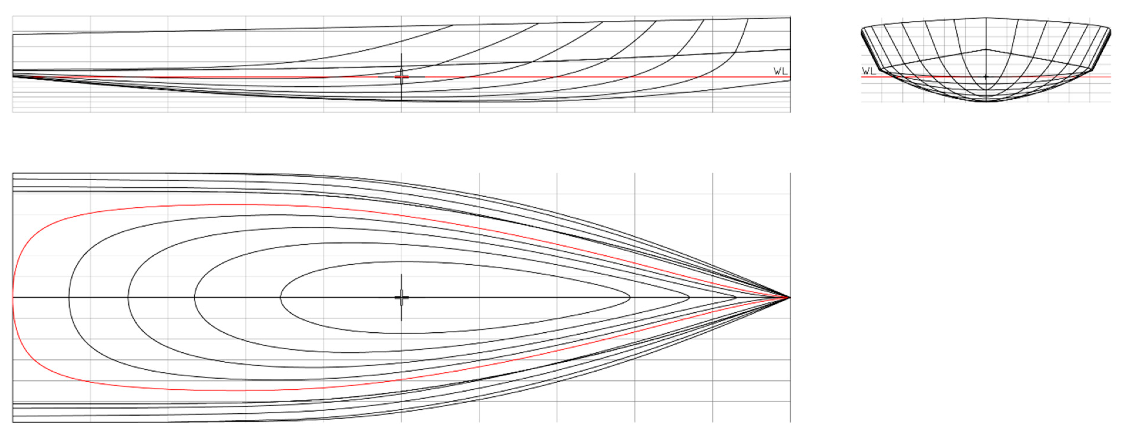
The 1001Vela Cup is an international competition where students from different universities design, build, and race their own skiff (a kind of sailboat, “sail, keep it fast and flat”) prototype. The class rules of this regatta are wide open and allow the designer to explore a huge selection of boat concepts with different hulls, sail plans, or even foil. These rules are defined by R3 class regulation and allow a maximum hull length of 4.60 m and a maximum beam of 2.1 m.

Thus, it is fundamental to model the hull, appendix, and sail geometry in accordance with marine conditions expected during the regatta, which every year is held in a different place; in this regard, CFD represents a useful tool to test with accuracy all the design options [14].

During the Midwinter Indoor Race, the hulls of the competitors is tested to evaluate which hull produces less drag for the whole set of speeds; during this race, designers can evaluate and compare the behavior and performance of different hulls and, most importantly, can validate the results of the hydrodynamic models they developed.

A special thanks goes to University of Napoli for providing free towing tank tests for all participants in the competition, thus providing the students with the opportunity to validate their work.

This paper is organized as follows. Section 2 gives a brief review of the skiff and its properties, as well as describing the Federico II towing tank facility. In Section 3, the numerical setup of the CFD model is explained, with details provided in the subsections. Section 4 concerns the presentation of the results and the comparison with the experimental fluid dynamics (EFD). Finally, in Section 5, conclusions are shown.

2. Materials and Model

2.1. Properties of Atka during the Midwinter Race

In this section, the characteristics of the hull of Atka (name of the boat) as it was tested are reported (see Figure 1).

Mass and inertia values are accounting for the two sailors that were on board during the regatta and for the full rig of the boat. In order to reproduce the real mass distribution during the experiment, the rig and the sailors were replaced with 18 small blocks of 9.722 kg. A schematic representation of the hull and its mass distribution is shown in Figure 2.

It is a good and widespread practice to place the reference system in the bottom part of the stern, with the x axis pointing to the bow, the y axis pointing inside the domain, and the z axis pointing to the top [1].

Atka’s hull properties are shown in

Table 1. Properties of Atka’s hull.

Displacement with Rig and Two Sailors (kg)	265
Center of Gravity (m)	(2.21259, 0.0, 0.28274)
Inertia Moments (kg × m2)	(38.464, 158.549, 183.495)
Water Line Height (m)	0.0442
Length Water Line (m)	4.60
Max Beam (m)	1.480

, and all the measurements are in accordance with the laboratory coordinate system just defined:

2.2. The Towing Tank of Naples University

The tank of Federico II is the largest in Europe supplied to a university and has the following dimensions: 136.74 × 9.00 × 4.25 m (length, width, depth), and on its sides, it has the sliding rails of a dynamometric carriage. At the end, an absorbing "beach" is present, which can reduce the amplitude of the incident waves by up to 95% for wavelengths between 5 and 7 m. The beach consists of a steel structure of appropriate curvature, 6 m long in the longitudinal direction, covered with PVC.

During the test, the boat is hooked up to the dynamometric carriage through two guides on the axis of the boat, one at the bow and the other at the stern, which restrict the boat in the y-direction and make it move forward in the x-direction, at the speed of test. These guides guarantee free motion along the two degrees of freedom of heave and pitch as shown in Figure 3.

Before each test starts, the acquisition system measures the hydrostatic conditions which will be used as a reference offset for the measurement of pitch and heave values. Then, the carriage is launched, and only after the transient acceleration phase, when the condition of uniform motion is reached, does the acquisition of running data begin.

In data acquisition, all measurements are temporal variables and therefore the basics of statistics are applied to obtain a summary of the data.

The dynamometric carriage is equipped with all the instruments necessary to measure dimensional quantities such as drag forces, motions, accelerations, speeds, inclinations, and temperatures. All these quantities are evaluated through the use of sensors which are in direct interaction with the measured system and transform the input signal into an electrical signal.

3. CFD Model

The analysis was carried out on the commercial software Star-CCM+ 2019.1 from Siemens [15]. The simulation setup was quite complex since the problem involved multiphysics and dealt with dynamic body motion. We used an Unsteady Reynolds Averaged Navier Stokes (URANS) CFD approach, which is considered to be an appropriate compromise between accuracy and computational cost for naval applications, according to consultancy companies and relevant bibliographies [16,17,18]. A time advancing approach was used in this work, even though the final solution was stationary, because the dynamic equilibrium position that the hull reached under different speeds was not known a priori, and the trim angle changed for the three different tests [19].

3.1. Domain, Boundary Condition, and Damping Factor

In fluid dynamic simulations of a towing tank test, it is not advised to use the real dimensions of the towing tank for the computational domain. In fact, it is only required that the boundary conditions do not influence the physics within the domain; thus, using the real tank for sizing the domain would be a waste of resources that would bring no benefit on accuracy [20].

However, the domain’s dimensions do have an important impact on the fluid dynamics and are linked to the speed of the test. It is fundamental to capture the wave pattern reasonably well, in order to evaluate the amount of energy that is subtracted from the boat. In this regard, the domain needs to be large enough to contain about 6 wavelengths behind the hull; in this way, it is possible to accurately compute the contribution to the total drag due to the perturbation of the wave field after the transition of the hull, usually referred to as wave-making resistance [13,14].

Another important aspect that influences the domain’s dimensions is wave reflection, which is undesirable and should be avoided.

The reflection problem is of crucial importance in both real towing tanks and numerical tanks. It is not possible to produce accurate and meaningful measurements when the tank or the computational domain is perturbed with reflected waves coming from all directions. This leads to bad measuring in real cases and/or simulation crash in the case of numerical tanks.

A simple approach is used to solve this issue in real and in CFD tanks: A large damping zone is introduced at the boundaries of the tank in order to absorb most of the energy of the incoming waves before they are reflected, hence leaving the domain undisturbed from reflection. In numerical simulations, the length and the intensity of this damping zone must be related with the domain dimensions, wavelength, and wave height. For our case, a damping zone of two times wavelength is enough to prevent wave reflection at boundaries [21,22,23].

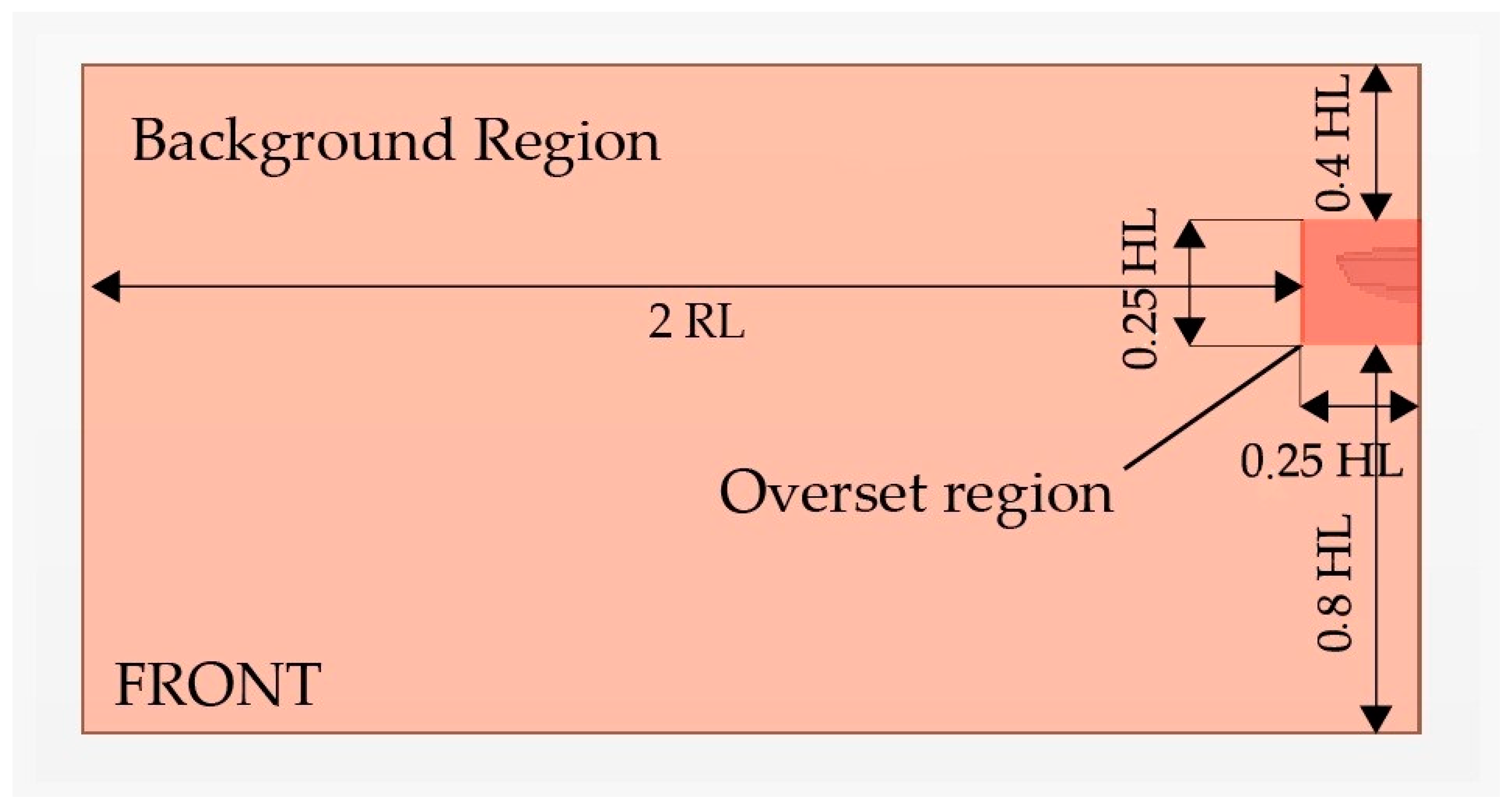
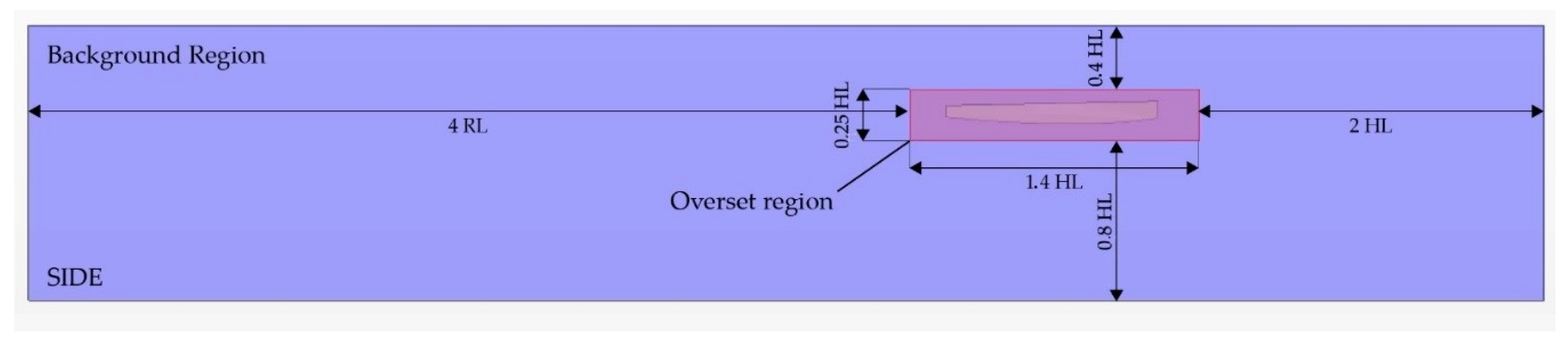
At this point, it is clear that a parametric approach represents the best choice in order to save computational time, where domain length, mesh refinement, damping zone, and other important parameters are functions of the wavelength and thus of the speed of test. In this regard, a reference length (RL), which is the longer length between hull-length and wavelength, was chosen, and the domain’s dimensions are a function of the reference length, as shown hereafter and in Figures 5 and 6:

(1)

Two hull-lengths (HL) in front of the boat;

(2)

Two reference lengths (RF) for the side;

(3)

Four reference lengths behind;

It is worth noting that the dimension in front of the boat is not parametric but fixed because waves do not propagate in that direction.

A damping zone of two wavelengths acting on outlet and side boundaries was added to these dimensions; intensity and length of damping was evaluated in accordance with [24].

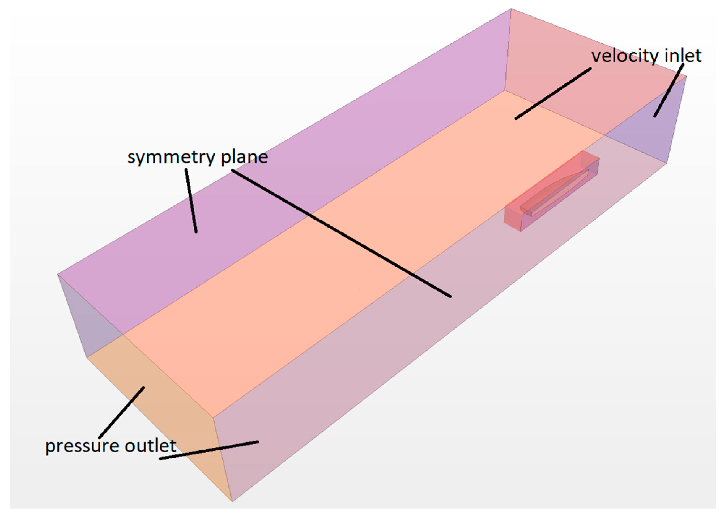
Following bibliography and the Star-CCM+ guidelines, boundary conditions were set as follows [20,25], and are shown in Figure 4:

(1)

Top and front are velocity inlets;

(2)

bottom and back are pressure outlets;

(3)

both sides are symmetry planes.

Figure 5 and Figure 6 show the dimensions of the overset and background regions:

3.2. Mesh Generation

The model deals with a moving body, because the final dynamic equilibrium position the hull reached under different velocities was not known a priori. In CFD, there are two ways to deal with a moving body: Mesh morphing/remeshing and overset mesh. Mesh morphing is better when the movements of the body are very small, so the cell quality does not decrease and few remeshing operations are needed. Overset mesh is used if, when dealing with large motion, a mesh morphing approach becomes unstable and too time-consuming due to several remeshing operations required. Using the overset approach, no re-mesh operation is needed because the mesh never deforms, nor does its quality decrease, since it moves with the body and remains unaltered [24,25].

A mesh morphing approach suited the application under consideration well, since the dynamic equilibrium was not far from the static one and there were incoming no waves that would induce large movements of the hull.

On the other hand, in order to deal with a head sea, the overset approach became necessary due to the large expected motion of the hull. Therefore, although there was no incoming wave in this study, an overset motion was implemented since the same CFD model can be used for further analysis to also comprise incoming waves [26].

The domain was thus divided into two separate regions: Background tank and overset.

The overset contained the moving part of the problem and allowed the boat to translate and rotate while the background remained fixed and unaltered. Equations were solved separately in the two regions and the solution was interpolated in an overlapping area consisting of cells called donors and acceptors, where information is exchanged. A linear interpolation scheme was used, even though it required a higher computational effort in respect to the other methods available, because it minimized interpolation errors and guaranteed better convergence and a more accurate solution.

While the dimension of the tank changed as a function of the test speed, the dimension of the overset was constant in all the simulations, because it referred to the moving body.

The meshing algorithm used in the two regions was different, as discussed in Section 3.2.1 and Section 3.2.2 for the tank and overset regions, respectively.

3.2.1. Tank

A trimmed block mesh was chosen due to the possibility to create anisotropic cells which best discretize the interface between the two fluids.

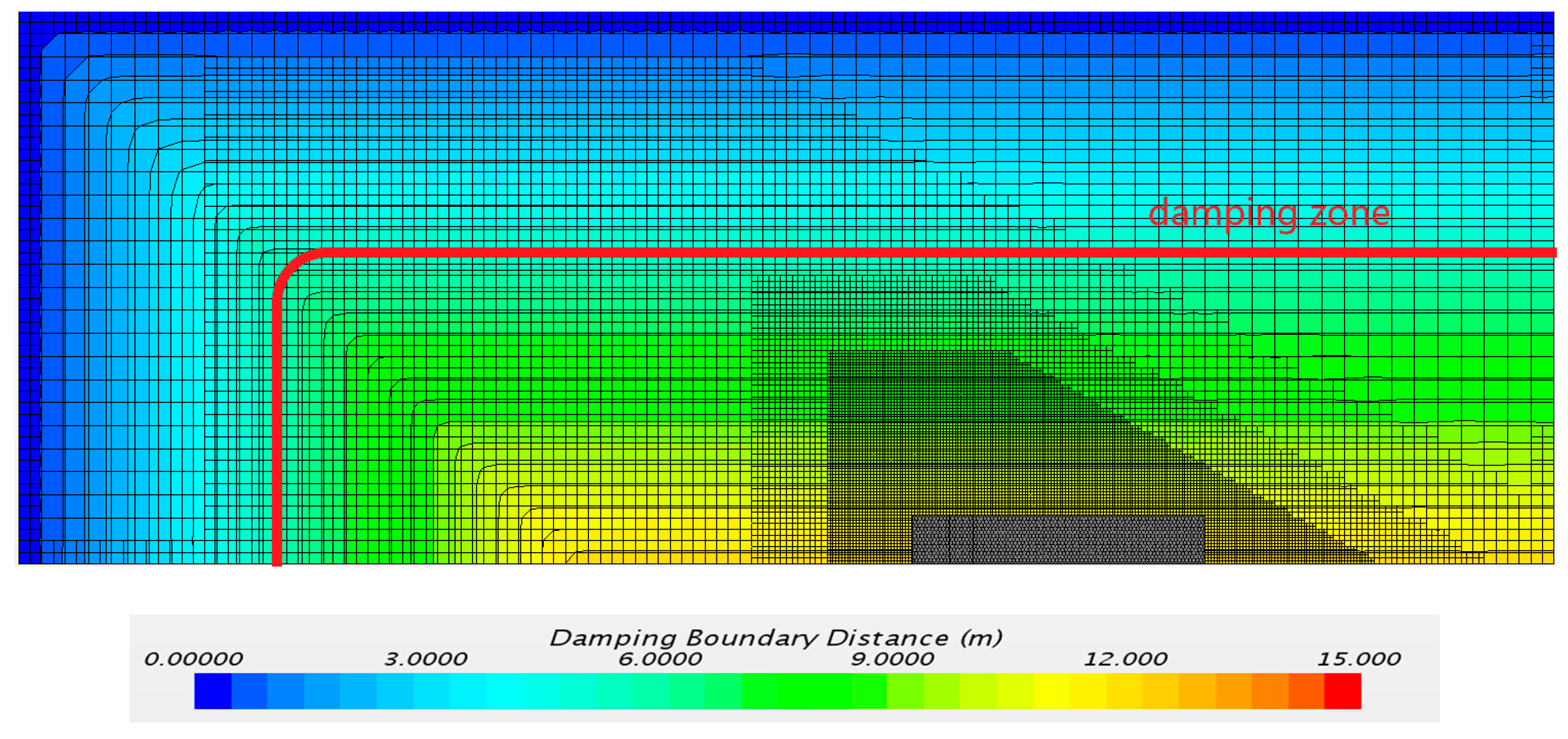
It is worthwhile to remark that wave reflection can occur, not only at boundaries, but also when the mesh size changes too abruptly [23,27]. To solve this problem, usually 2 or 3 different volumetric refinements are used to gradually coarsen the mesh at sea surface, from the near wall zone to the far field. The artificial damping of waves should start before the coarsest grid starts, since such a change in cell size is a potential source of reflection that has to be included in the damping zone. Therefore, wave damping should start where the mesh is still fine, but not too close to the hull, in order to avoid any influence on the wave pattern [23]. The mesh refinement regions, as well as the damping zone, are shown in Figure 7.

When dealing with trimmed mesh in Star-CCM+, it is important to bear in mind that cells can only double or half their size; so, starting from the inner and finer volumetric control for the sea surface and doubling up dimensions, we used this distribution of cells: 20 cells to discretize the wave produced by the hull, with an aspect ratio between x/y and z dimensions of 4:1 (because the waves were not too steep) [28,29].

Moreover, to prevent wave reflection at the interface between the overset and background mesh, cells at the interface had an aspect ratio of 2 in order to facilitate communication between the two regions. The volume of the cells at the interface had to be comparable to obtain good results and prevent a simulation crash.

3.2.2. Overset

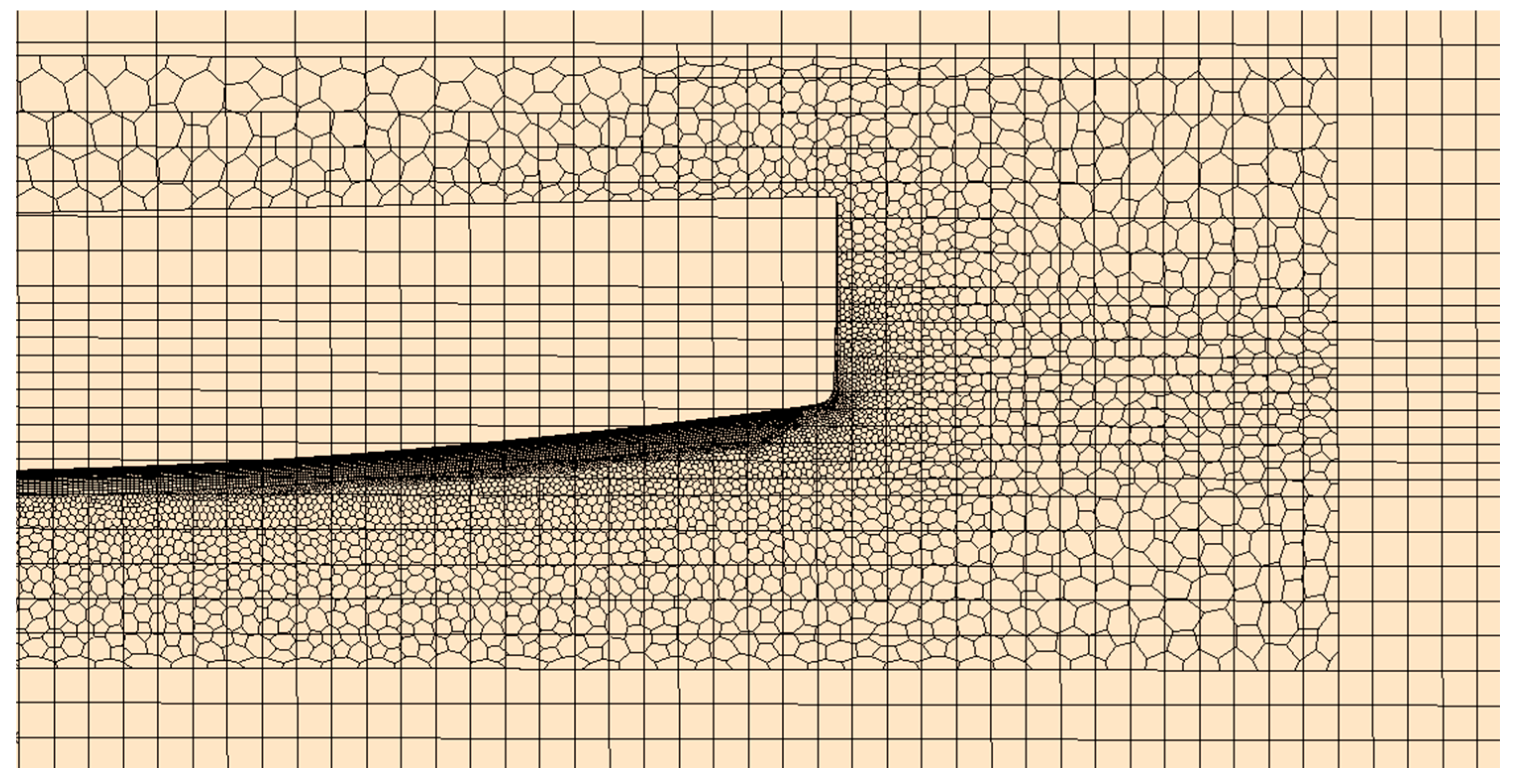
A polyhedral mesh was chosen for the overset region, as shown in Figure 8, due to the possibility to change the volume of cells gradually and prevent wave reflection near the boat where the strongest gradients are solved.

To better capture the pressure gradients and wave generation at the bow and stern, volumetric refinement controls were applied in order to reduce mesh size in these areas: A control at the bow with very fine cells was used to avoid numerical ventilation [30], and a control for the stern guaranteed the correct flux under the hull.

When deciding for the overset dimensions, two main aspects should be considered:

(1)

Overset does not have to be excessively large, otherwise even small rotations may induce large movements and increase the probability of interpolation errors;

(2)

neither should it be too small, because cells need some space to grow from the wall to a decent size in order to maintain a low element count.

3.3. Volume of Fluid

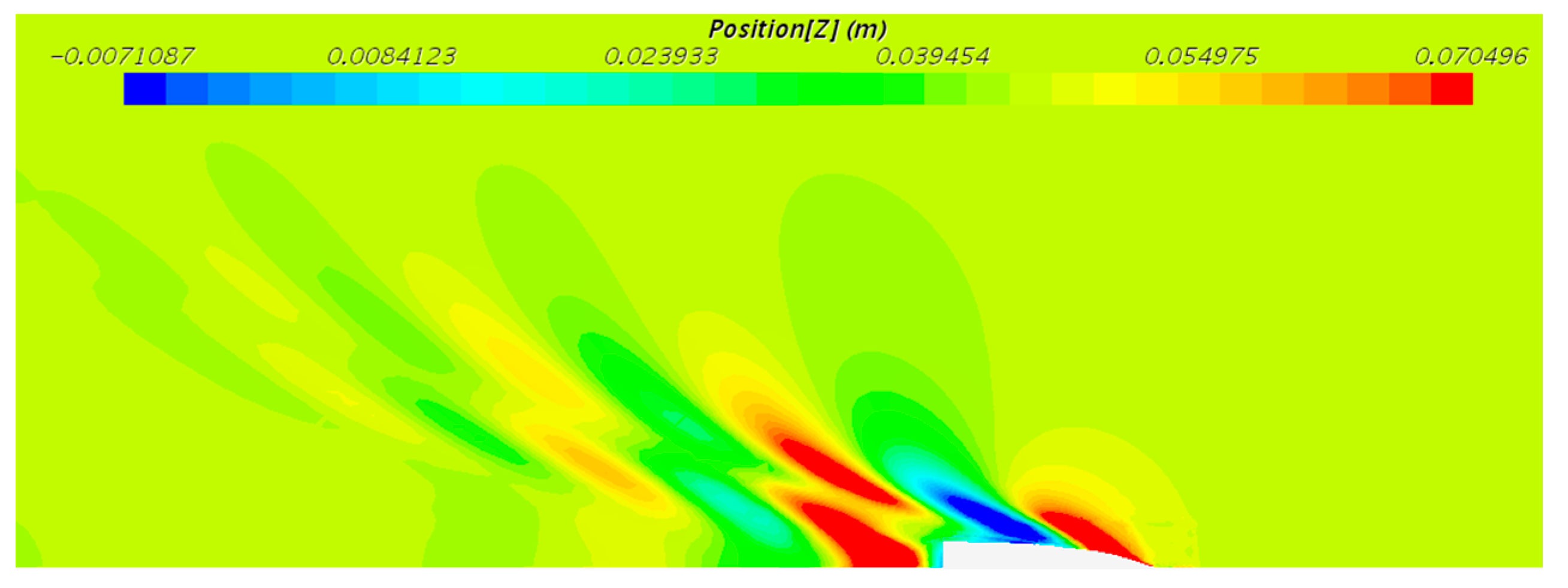
The volume of fluid (VOF) multiphase model is a simple multiphase model. It is used to solve problems involving immiscible fluid mixtures, free surfaces, and phase contact. Figure 9 represents the elevation of the free surface in respect to the laboratory reference system, and shows how the VOF model is able to track difference phases and thus define the wave pattern behind the hull.

Due to its numerical efficiency, the model is suited for simulations of flows wherein each phase constitutes a large structure, with a relatively small total contact area between phases [31].

The spatial distribution of each phase at a given time is defined in terms of a variable that is called the volume fraction. A method of calculating such distributions is to solve a transport equation for the phase volume fraction. The method uses the STAR-CCM+ segregated flow model [32].

By default, the VOF free surface calculation is performed during the same time step as the other calculations. To ensure simulation stability, at free surface the value of CFL (Courant–Friedrichs–Lewy number) must be limited to 1, and better results with a sharp resolution of the two phases are obtained with a CFL around 0.5 [28,29]. However, such a limitation is overly restrictive, as other physics calculations with implicit solvers can run at a much larger CFL number. This reduces the computational efficiency of VOF free surface simulations.

The multi-stepping feature removes this limitation on the CFL number; this option applies temporal sub-cycling to the transport of volume fraction and can improve the resolution of the interface between two phases; however, multi-stepping cannot be used with second order time discretization in Star-CCM+.

To maintain the accuracy that only a second order time scheme can guarantee, the multi-stepping feature has been disabled; thus, the value of CFL at the interface between phases represents a real and strong limitation for the time step of the model.

3.4. Dynamic Fluid Body Interaction (DFBI)-6DoF Solver

The dynamic fluid body interaction (DFBI) module simulates the motion of a rigid body in response to forces exerted by the physic continuum.

The 6-DoF (degree of freedom) solver computes fluid forces, moments, and gravitational forces on a 6-DoF body; pressure and shear forces are integrated over the surfaces.

For time integration, the 6-DoF solver employs a trapezoidal scheme of second order accuracy. This is independent of the order of accuracy of the implicit unsteady solver for the momentum and continuity equations.

When working with body motion, it is convenient to provide a smoothing ramp, so that forces on the hull are released meekly and not impulsively.

If no ramp is set up, abrupt impulses generate both physical and numerical transients and oscillations that affect the kinematics of the floater, which damp out several seconds after the beginning of the simulation [30,31,33].

Therefore, although the additional ramp time must be added to the simulation, the computational time is shorter due to a faster and cleaner convergence.

We decided on a release time of one second and a ramp time of two seconds: The moving body remained fixed in all DoFs for the first second of the simulation, in order to allow the fluid field around the floater to assume more realistic values in respect to initialization with a constant speed all over the domain; then from seconds 1 to 3, all the forces were smoothly applied to the body until the full value was used when ramp time ended at 3 s. The simulation results converged 6 seconds after the end of the ramp time; thus, the total time simulated was 9 s, which was enough to fully develop the wave pattern behind the boat and to stabilize drag and trim reports to constant values.

3.5. Turbulence and Law of the Wall

The flux around the hull was fully turbulent since the Reynolds number was in the order of millions; thus, turbulence had to be modeled to accurately compute forces acting on the boat.

The K-epsilon model is recommended in VOF simulations as the computational cost is low and the accuracy in the discretization of the interface between the two phases is good enough [31,34].

In the present case, a realizable K-Epsilon model was used, which represented an upgrade of the standard model: A new transport equation was used for the turbulent dissipation rate; moreover, the turbulence viscosity was expressed as a function of mean flow and turbulence properties instead of being constant.

A two-layer wall treatment was used in combination with the realizable K-Epsilon model.

In this approach, the turbulence quantities were computed as a function of the wall distance in the near wall region, and evaluated solving the transport equation in the far field; values were smoothly blended between these two zones.

The two-layer approach allowed the use of different values for Y+ because it applied wall treatment when the mesh could not accurately solve the boundary layer, and solved without wall functions when the mesh was fine enough to discretize the sub-viscous layer near the wall.

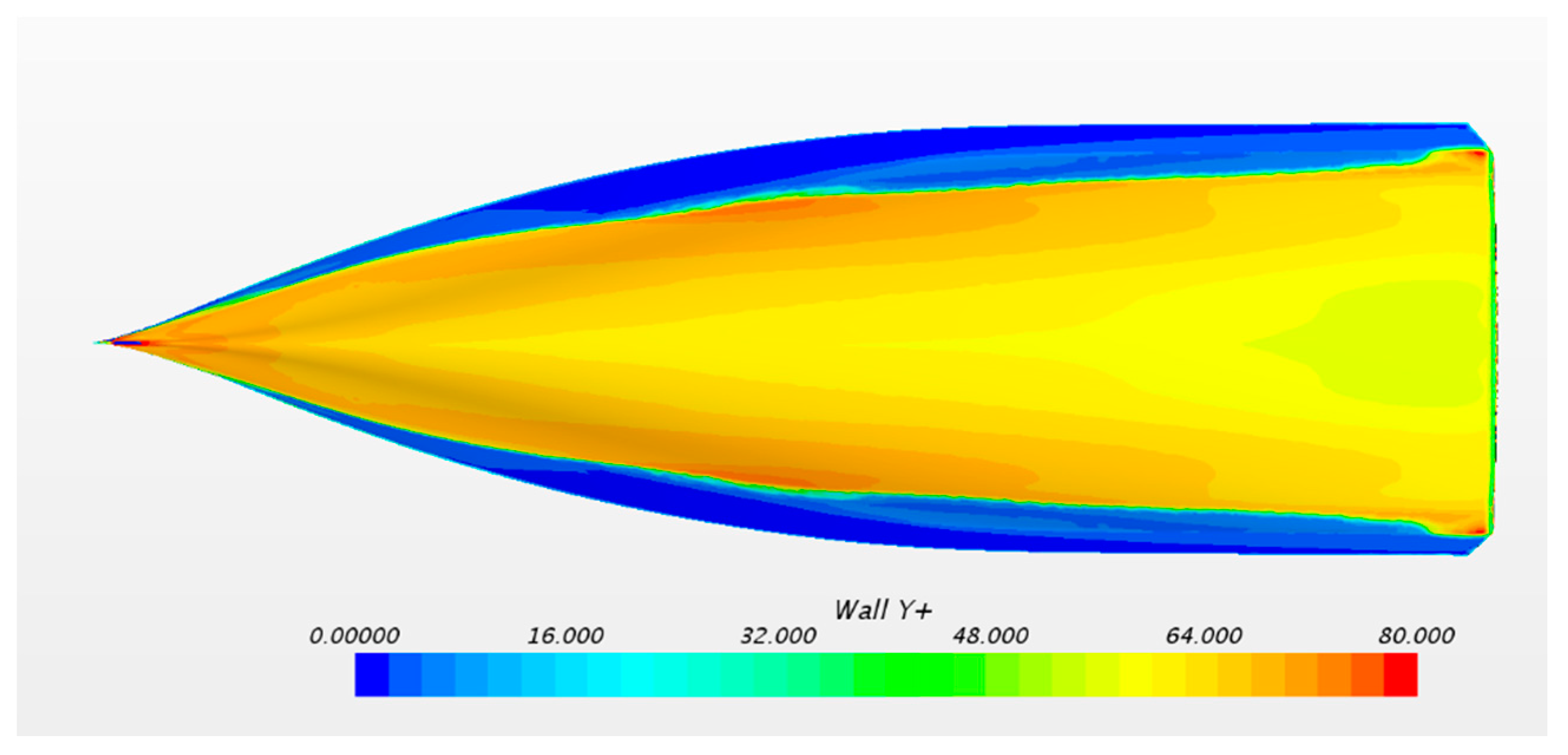
The hull is designed with a hydrodynamic shape in order to disturb the flow around it as little as possible; thus, phenomena like vortex shedding and fluid vein detachment do not occur, at least not for the range of speeds tested. This made it possible to discretize the region near the hull with a coarse mesh. In fact, if the fluid remained attached to the wall, there was no need to finely mesh the sub-viscous layer; however, values of Y+ around 50 (first cell in the logarithm layer zone) or more could be used (Figure 10) [35].

The discretization that guaranteed these Y+ values was the following: Thickness of the first cell for the 3 m/s simulation was 1 mm; 12 layers were used with a smooth growth factor of 1.2.

The thickness of the first cell near the wall changed for every simulation, in order to always aim for the same Y+ values when the speed changed.

3.6. Time Discretization

In Star-CCM+, the multiphase VOF solver requires an implicit time scheme and is not available when an explicit time scheme is used. Thus, a second order implicit time discretization was chosen because the first order was numerically diffusive, and the property of the waves was not transported correctly [32,33]. As a consequence, if a first order is used, waves behind the hull are significantly damped out a few meters behind the boat and the wave pattern results are much smaller than in real experience.

Time step for an implicit time scheme can be high because implicit is unconditionally stable; the CFL factor can be up to 10 and even more, while for an explicit approach, the CFL factor has to be below 1, otherwise the method becomes unstable. Nevertheless, when dealing with multiphase models and overset technology, two additional limitations must be satisfied:

(1)

The CFL number at the interface between the two fluids has to be at least less than 1 and it is suggested to keep it less than 0.5 in order to have a clean separation of the two fluids and a sharp interface [28,29];

(2)

the movement of the overset cells at the interface between the two regions must be less than half of the minimum cell size to prevent overset mesh crash errors due to the exchange of information [36].

The second condition is very important when simulating a hull in head sea and when deciding about the overset dimensions. The more severe limitation on the time step comes from the former, so the time step is a function of the speed of the test in order to aim for the same CFL at the sea surface. The time step goes from 0.01 s for 1 m/s test, to 0.0033 s for the 3 m/s test, and it scales linearly with speed.

3.7. Numerical Ventilation

In the case of planing hulls, for very high speeds, phenomenon of ventilation can occur: A thin film of air gets caught between the hull and the water, drastically reducing the drag. This is a well-known phenomenon often exploited to improve the design of high-speed planing motor yachts to reduce the viscous drag with water. Ventilation requires a speed of an order of magnitude greater than the speeds tested; therefore, it was not tested in the real experiment, nor will the sailboat ever experiment with it.

However, the numerical model can suffer from numerical ventilation [7,8,37], even for low speed such as 3 m/s (Froude number = 0.4465), for particular hull shapes or trimming angle, especially if the bow is not piercing the sea surface but lies over it [12,13], as shown in Figure 11.

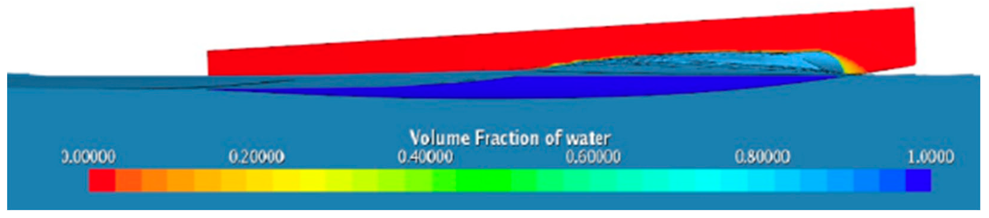
When implementing a dual phase simulation, due to the numerical interpolation method in the VOF model, it is possible that a fraction of air gets caught and remains trapped under the hull, creating a mixture of phases [30], as shown in Figure 12. Air usually undergoes the hull at the bow and travels down to the stern, establishing a steady flux. As a consequence, the wall friction drag is underestimated. It is worth remarking that the contribution of the form drag to the overall drag is not affected by numerical ventilation.

In order to solve numerical ventilation related problems, in this work, two approaches are used:

(1)

The first approach is related to the refinement of the mesh near the interface between water and air in the aft part of the bow. Here, an isotropic mesh is also used for the sea surface because an anisotropic mesh is more subject to numerical ventilation. This treatment works best when paired with the high-resolution interface capturing (HRIC) scheme designed to mimic the convective transport of immiscible fluid components, and is thus suited for tracking sharp interfaces [37].

This approach requires the CFL number in the target region to remain low; therefore, the computational cost increases because a very small time step is required. Furthermore, increasing the number of inner iterations in the implicit time-stepping scheme can reduce the likelihood of numerical ventilation; however, this numerical phenomenon remains dependent on the shape of the hull, trim angle, and speed of test, and may not be completely solved with this approach:

(2)

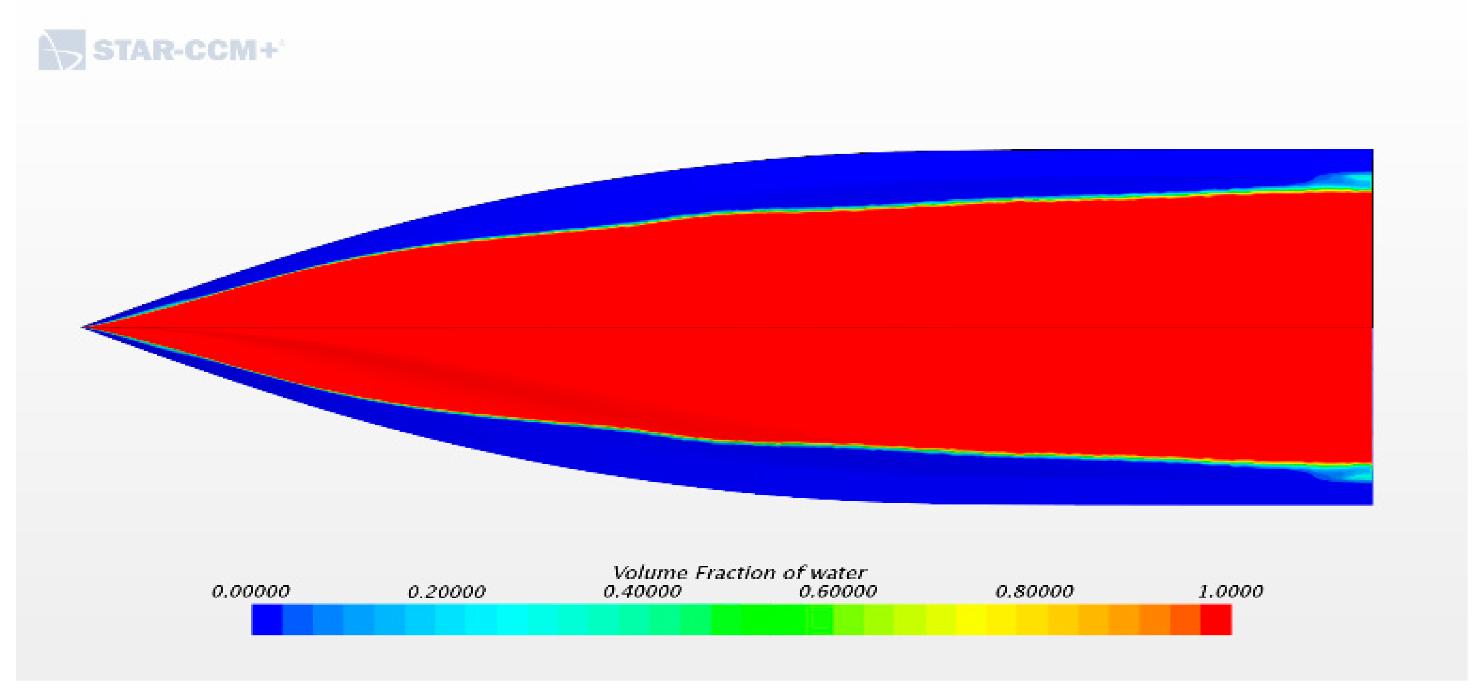
The second method, used to completely resolve the numerical ventilation problem, is the phase-interaction substitution procedure. After the simulation is converged to a certain draft and trim angle and the wave pattern is well established around the hull, a phase interaction is applied which substitutes all fluid zones that contain mixed phases with water.

This procedure consists of the following steps:

(a)

A scalar-user field function aiming to calculate all zones in the domain with a volume fraction of water higher than 0.5 is created;

(b)

the phase-interaction procedure is applied setting the user field function created at preceding point as the input; and the mixed phase is replaced with water;

(c)

the first order time accuracy must be set (because VOF phase replacement is not compatible with the second order time scheme);

(d)

only a single time step can be running to obtain the final result after the substitution procedure. If more steps are run, the water level keeps rising for each iteration because at sea surface there is never a sharp separation between phases; thus, a step after the other, the water occupies more and more volume. This also explains why it is important that the simulation is already converged to final values.

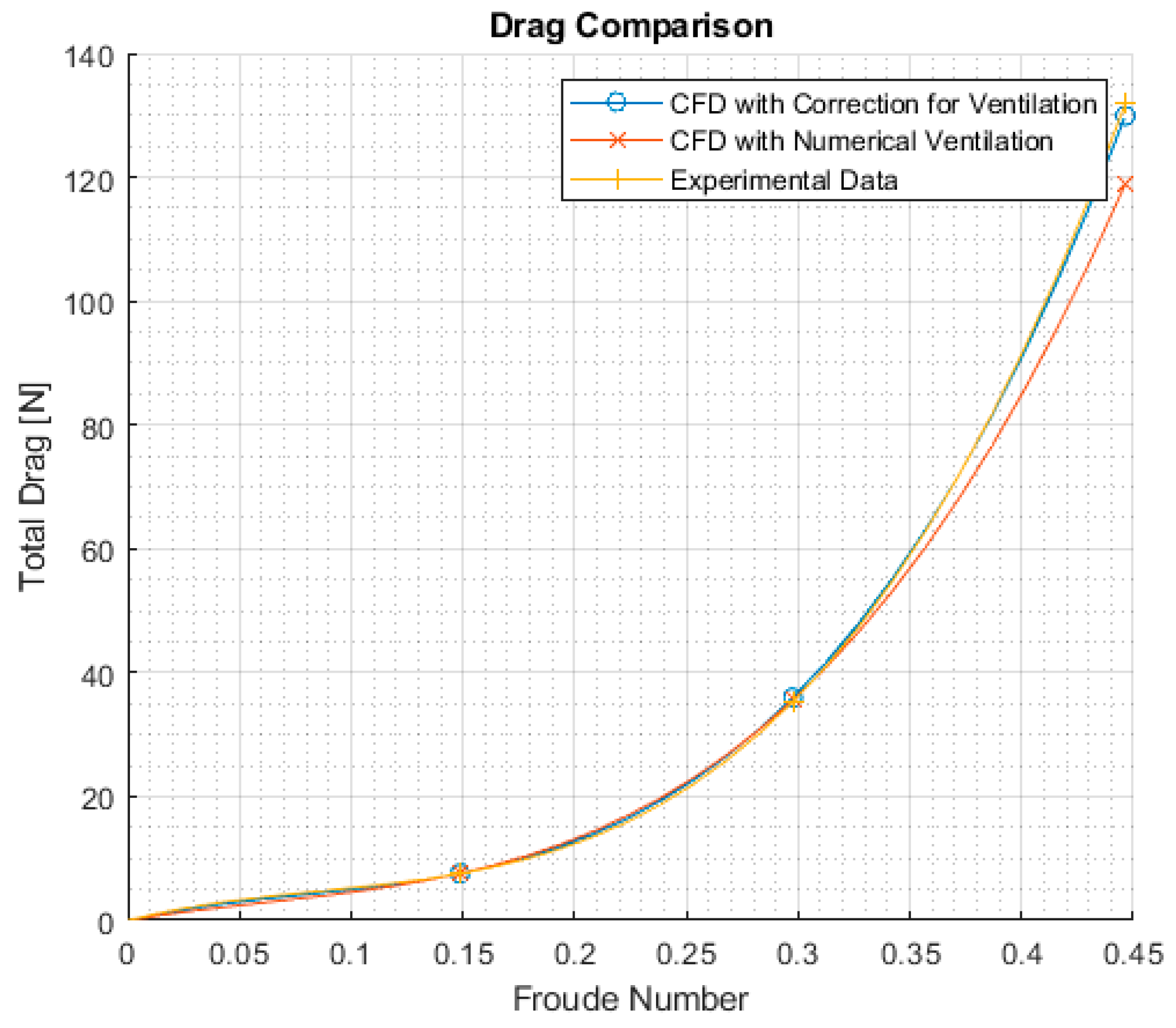
The correct shear stress was computed, and the real wetted surface was used without changing the physics of the problem. This technique allowed for a higher time step and a coarser mesh, especially at the wall in the bow part. Numerical ventilation was solved and all the forces acting on the hull were computed correctly, as shown in Figure 13. The second approach was preferred because it worked well in a calm sea simulation and granted a faster solution than that of the first method.

3.8. Convergence Study

Convergence study has key importance in every CFD simulation. This process proves that the discretization error has small influence on the result and that the solution will not change when refining the mesh. Convergence study allows the analyst to choose the best cell size, which represents an appropriate compromise between accuracy and computational speed; thus, it represents an opportunity to quantify the increment with an accuracy that a finer model would obtain, and compare it with the increase in central processing unit (CPU) hours required, as shown in Table 1.

Four different base sizes (the parametric value with which all the mesh is scaled) are investigated, associated with different cells’ count: Halving the base size generates a number almost 2³ times higher, since 3D volume cells are considered. When investigating grid convergence, it is important not to change other models and parameters, otherwise it would be impossible to discern what caused the different behavior in the simulation. This means scaling the time step for every different mesh size in order to maintain a constant CFL number. Similar considerations apply to the Y+ value, which must remain constant in all the simulations.

Therefore, a fixed value for the thickness of the first cell near the wall is used (when changing base size, not when changing the speed of the test), and the time step is scaled to maintain the same CFL for all the grids tested [38]. It is important to notice that simulation time increases significantly using the finest grid. This is not only due to the higher number of cells, but also to the smaller time step.

Table 2. Convergence study and comparison with experimental data for the 3 m/s test.

Base Size	Cell Count (Millions)	Total Drag (Half Hull) (N)	ΔTrim (Degrees)	ΔTranslation z (mm)	Relative Error Drag	Relative Error ΔTranslation z	Relative Error ΔTrim	Computational Time
Experimental Data	-	66	0.878	18.6	0	0	0	-
0.667	2.2	65.34	0.871	18.8	1.00%	1.08%	0.80%	36 h × 16 CPU
1	1.01	65.24	0.892	19.103	1.15%	2.70%	1.59%	12 h × 16 CPU
1.5	0.62	64.94	0.901	19.846	1.61%	6.70%	2.62%	6 h × 16 CPU
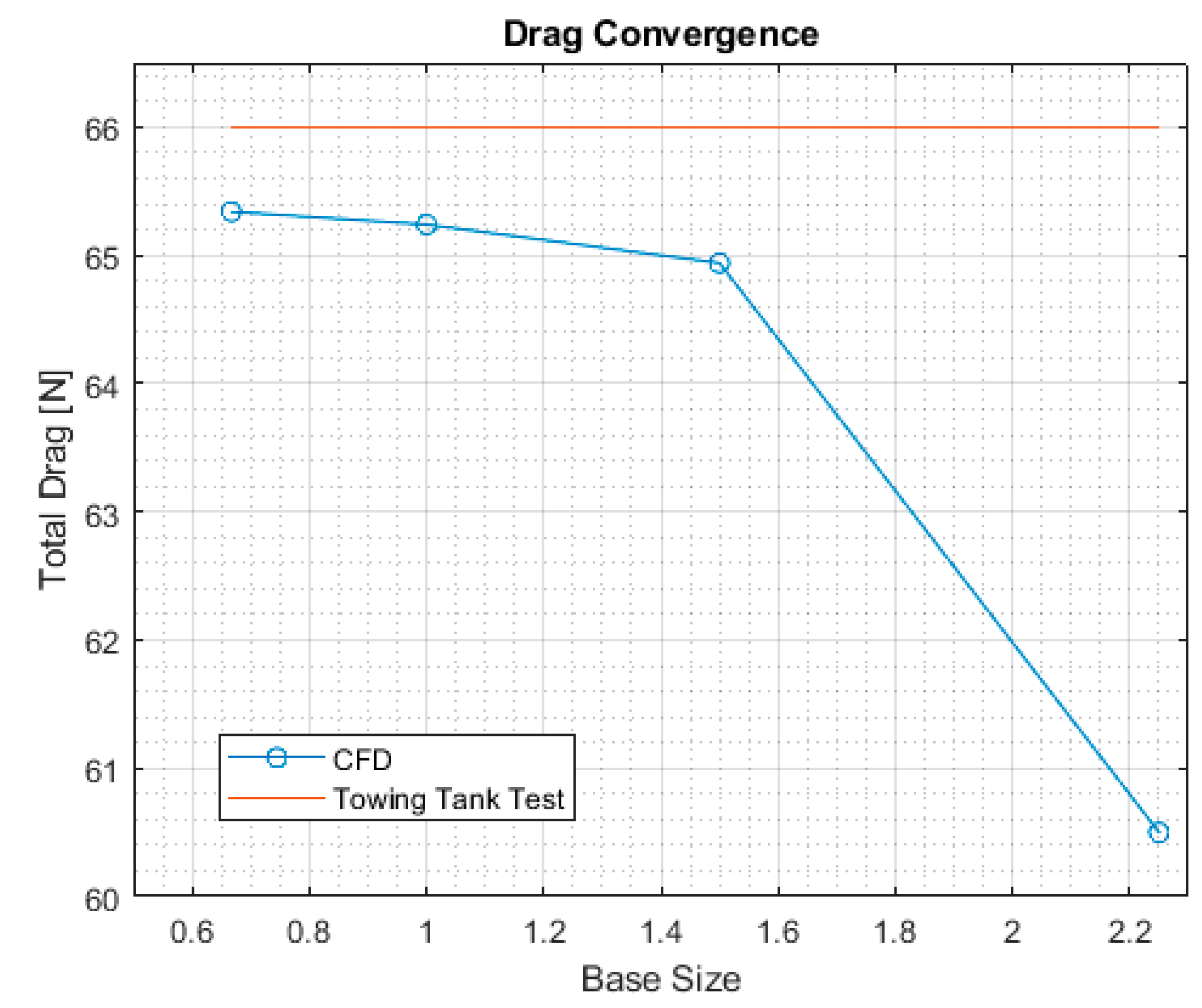
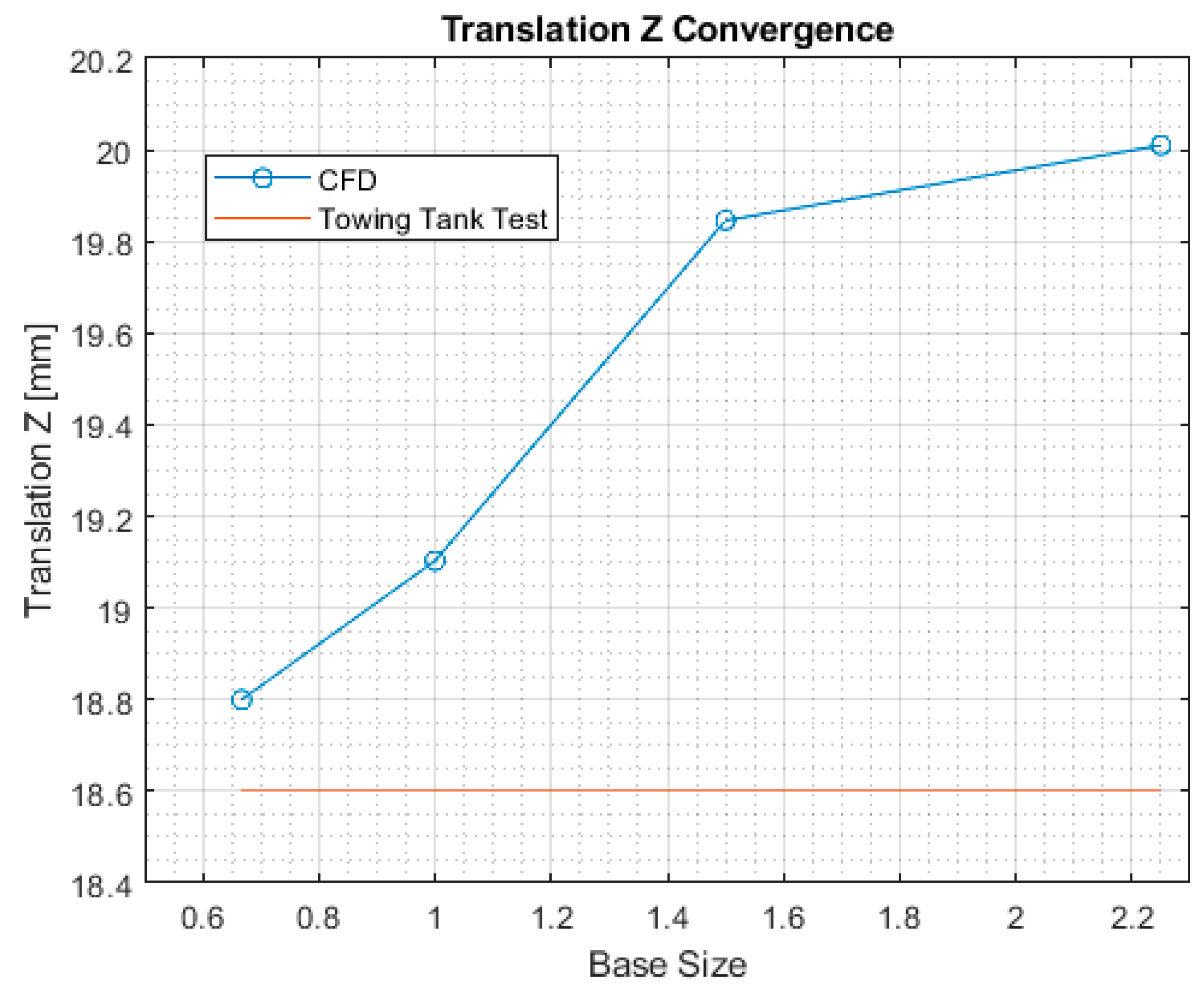
2.25	0.5	60.5	0.935	20.01	8.33%	7.58%	6.49%	4 h × 16 CPU

presents the different base sizes used, the associated number of cells, the relative errors, and the corresponding CPU time of the simulation. The physical quantities that were monitored in this convergence study are the total drag experienced by the hull, the translation along the z axis, and the trim angle. The obtained total drag and vertical translations are shown in Figure 14 and Figure 15, respectively. The benchmark used to build the error metrics is the dataset from the EFD. The method used for the analysis is the Richardson extrapolation, with the correction based on the total number of cells [39]. In this regard, the base size had to have a constant increment; in order to keep the cell count low, we decided for 1.5 as the multiplier for the base size.

As shown in Table 2, the mesh resulting from the base size equal to one was chosen, since it achieved errors similar to the finest mesh, while computing 3 times faster. Further refinement of the mesh would not significantly increase the accuracy of the simulation but would make it more expensive.

4. Results: Comparison between CFD and EFD

Results in

Table 3. Comparison between experimental fluid dynamic (EFD), computational fluid dynamic (CFD) with numerical ventilation, and CFD after correction.

Froude Number	Velocity [m/s]	CFD Drag (Numerically Ventilated) (N)	CFD Drag Post Correction (N)	TTT Drag (N)	Relative Error (Corrected Drag vs. EFD)	ΔTrim Angle CFD (°)	TTT ΔTrim Angle (°)	Relative Error (CFD ΔTrim vs. EFD ΔTrim)
0.1488	1	7.58	7.60	7.55	0.61%	−0.248	−0.254	2.3%
0.2977	2	35.6	36.0	35.3	1.94%	−0.613	−0.622	1.4%
0.4465	3	119	130.48	132	1.13%	0.892	0.878	1.5%

are obtained from the postprocessing of CFD simulations and are presented in Figure 16 and Figure 17. The main objective of this work was to validate the numerical model through comparison with experimental data. Furthermore, it is interesting to compare results with and without correction for numerical ventilation in order to evaluate the benefit of the numerical strategy herein proposed. Values of ΔTrim angle were positive when the bow was lifted up.

As clearly shown in Figure 16, experimental results are better approximated when the numerical ventilation correction is applied. This method increased the total advancing drag of the hull and guaranteed a reduction of the relative error with respect to the experimental data; the error of the numerical model after correction was between 0.61% and 1.94% for drag, below the 2% threshold. The difference after ventilation correction was noticeable only for 3 m/s because for the other two speeds tested the numerical ventilation under the hull was practically absent. Moreover, it is important notice that the ventilation correction did not influence the trim angle at all, leaving it unchanged.

5. Conclusions

Considering the results that emerged from this work, the advantages of the CFD model have been confirmed. Numerical RANS simulation represents an accurate mean for the test of a new hull and can be useful during the boat design and testing process. This work aimed to group all the best practices that should be implemented during a CFD study of a hull in calm sea conditions, and represents the starting point for future studies regarding motion in head sea. Two different methodologies dealing with numerical ventilation, which can also occur for low speeds such as 3 m/s, were presented in this paper. The goal of having a fast and accurate simulation, and of solving the numerical ventilation problem, was achieved using the second methodology proposed, which fits perfectly for cases in which speed is low and no real ventilation occurs. It is worth noting that the phase substitution procedure cannot be used when the ventilation is both real and numerical because this method completely removes air from the bottom of the hull; therefore, the technique proposed here should not be used for high-speed planing crafts.