The Use of Geographic Databases for Analyzing Changes in Land Cover—A Case Study of the Region of Warmia and Mazury in Poland


Abstract
:
1. Introduction
1.1. Land Cover and Landscape Fragmentation
1.2. Sources of Data on Land Cover
- acquire and synchronize interdisciplinary data on the state of the environment with the main focus on priority areas in each Member State of the European Community;
- harmonize and coordinate the organization and management of data at the local and international level;
- guarantee the compatibility of the gathered data.
2. Materials and Methods
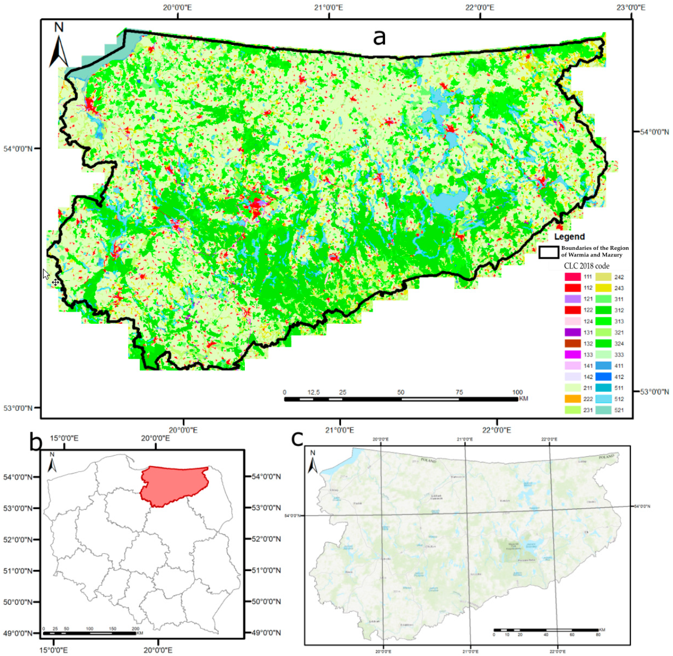
2.1. Study Area
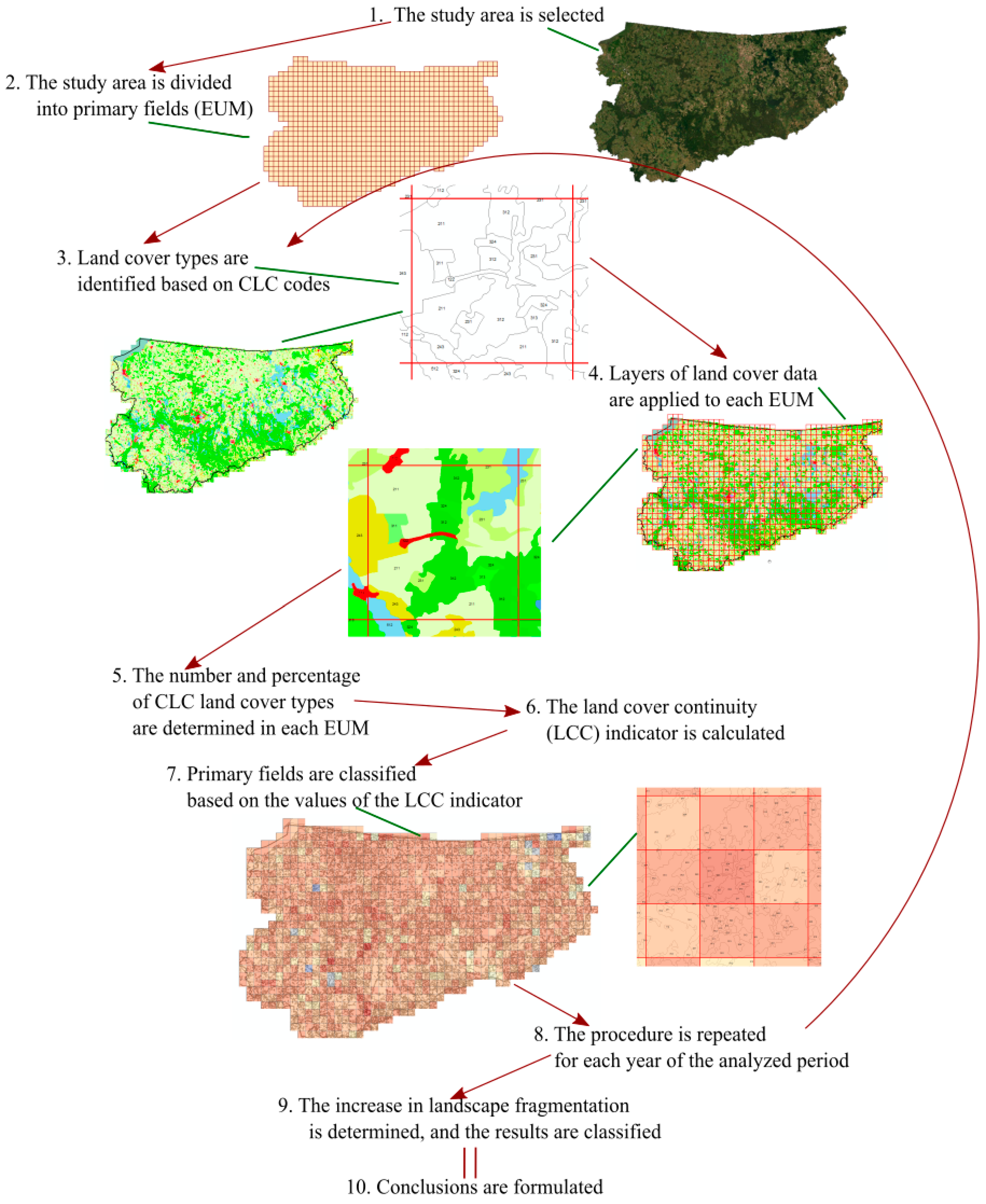
2.2. Procedure
- LCC—indicator of land cover continuity;
- n—equivalent unit of measurement (EUM);
- LSC—proportion of the ith land cover type in the EUM;
- m—number of land cover types in the EUM.
2.3. Data
- Urbanized areas—developed areas, including residential, commercial, and industrial areas, mines and green areas in cities.
- Agricultural areas—all categories of agricultural land, such as arable land, pastures, meadows as well as farmland covered by native vegetation.
- Forests and semi-natural areas—forests, areas covered by trees and shrubs, as well as open areas with little or no vegetation in forest systems.
- Wetlands—this category includes land that is highly saturated with water, including marshes, swamps, peat bogs, as well as intertidal flats and salt marshes.
- Water bodies—marine and inland waters.
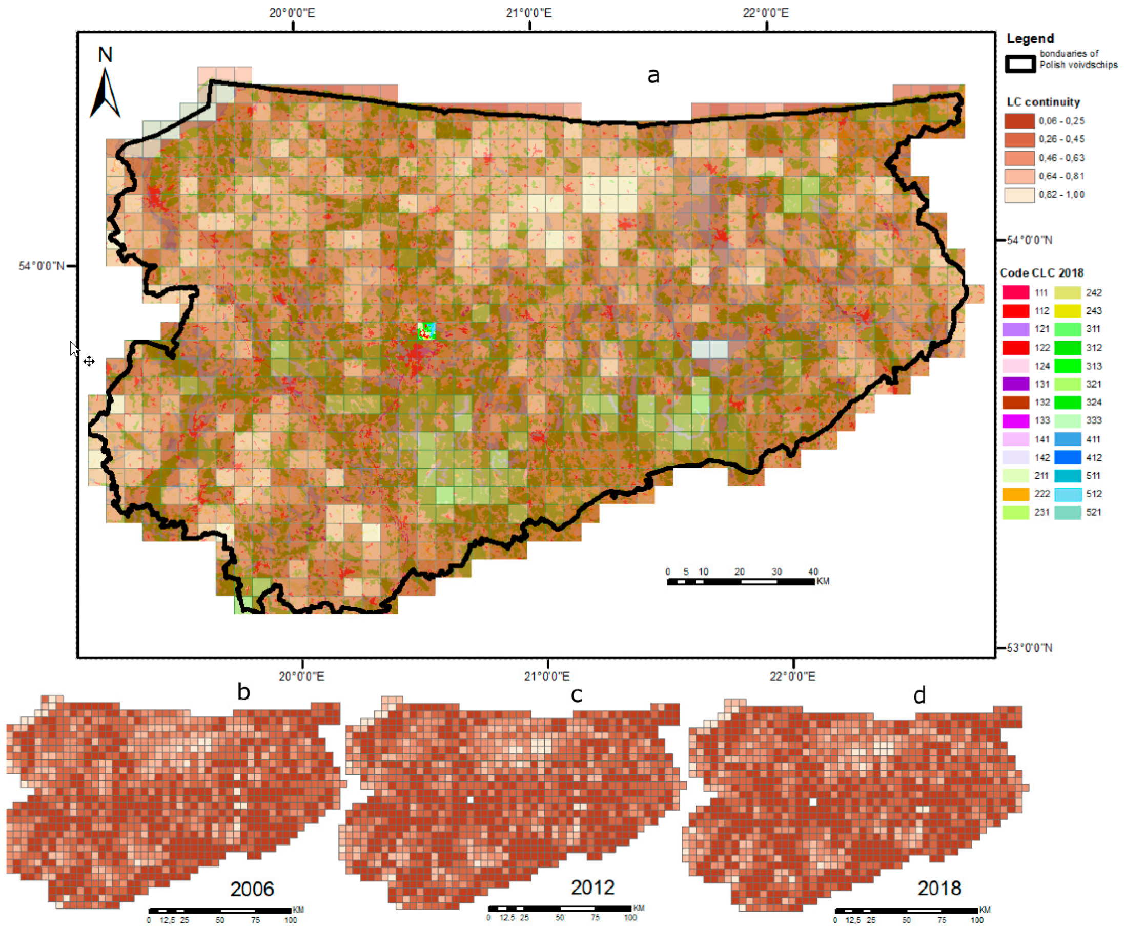
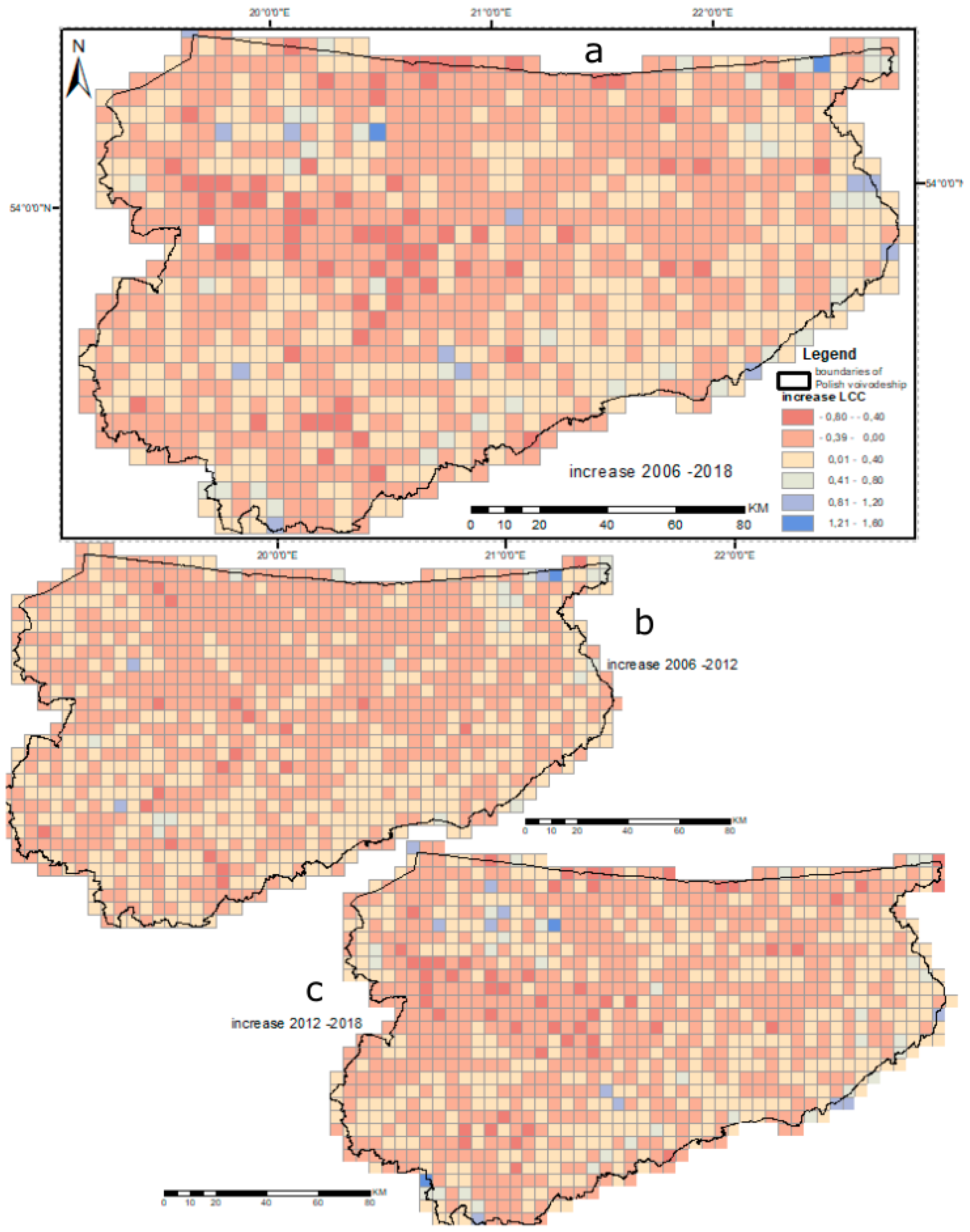
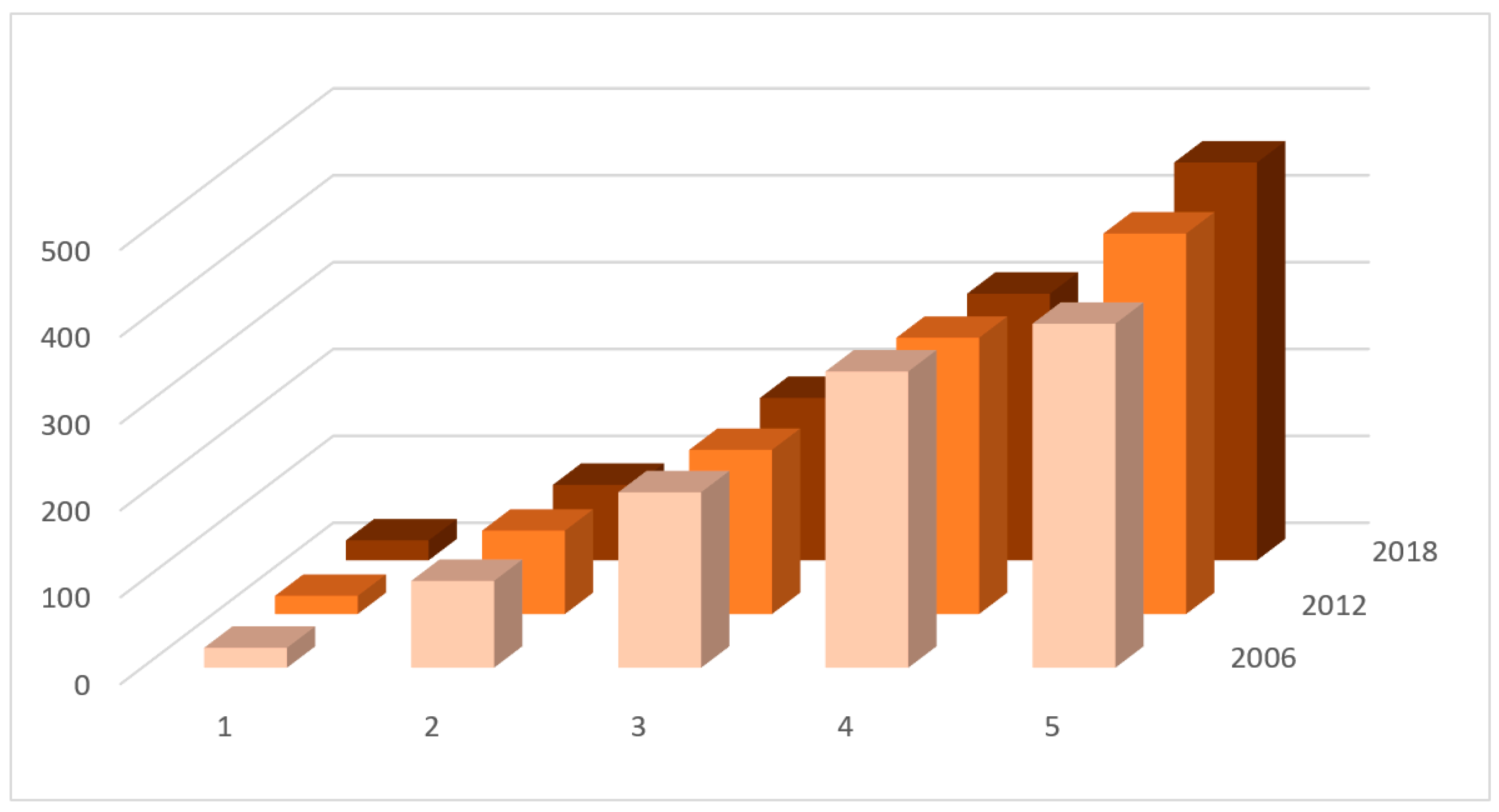
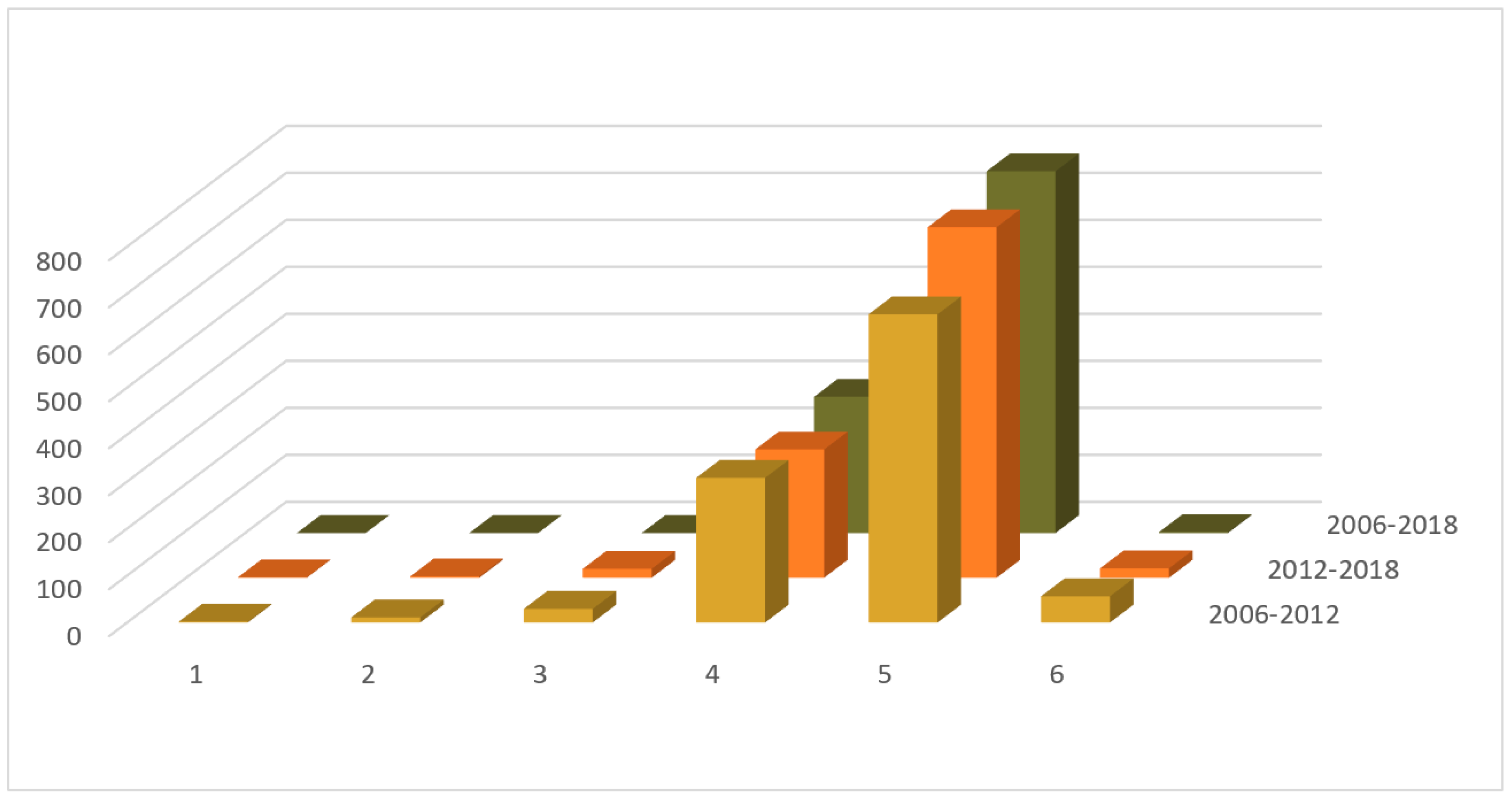
3. Results
4. Discussion
5. Conclusions
Author Contributions
Funding
Conflicts of Interest
References
- Wei, T.; Shangguan, D.; Shen, X.; Ding, Y.; Yi, S. Dynamics of Land Use and Land Cover Changes in An Arid Piedmont Plain in the Middle Reaches of the Kaxgar River Basin, Xinjiang, China. ISPRS Int. J. Geo-Inf. 2020, 9, 87. [Google Scholar] [CrossRef] [Green Version]
- Pelorosso, R.; Leone, A.; Boccia, L. Land cover and land use change in the Italian central Apennines: A comparison of assessment methods. Appl. Geogr. 2009, 29, 35–48. [Google Scholar] [CrossRef]
- Cieślak, I. Multifaceted Analysis of Land Use Conflict; Wydawnictwo UWM: Olsztyn, Poland, 2018. (In Polish) [Google Scholar]
- Cieślak, I.; Szuniewicz, K. The quality of pedestrian space in the city: A case study of Olsztyn. Bull. Geogr. Socio-Econ. Ser. 2015, 30, 31–42. [Google Scholar] [CrossRef] [Green Version]
- Wubie, M.A.; Assen, M.; Nicolau, M.D. Patterns, causes and consequences of land use/cover dynamics in the Gumara watershed of lake Tana basin, Northwestern Ethiopia. Environ. Syst. Res. 2016, 5. [Google Scholar] [CrossRef] [Green Version]
- Petrisor, A.-I.; Sirodoev, I.; Ianos, I. Trends in the National and Regional Transitional Dynamics of Land Cover and Use Changes in Romania. Remote Sens. 2020, 12, 230. [Google Scholar] [CrossRef] [Green Version]
- Büttner, H. The Stakeholder Dialogue in the Third Project Phase of GLOWA-Danube. In Regional Assessment of Global Change Impacts; Springer Science and Business Media LLC: Berlin/Heidelberg, Germany, 2016; pp. 49–53. [Google Scholar]
- Soto-Berelov, M.; Madsen, K. Continuity and Distinction in Land Cover Across a Rural Stretch of the U.S.-Mexico Border. Hum. Ecol. 2011, 39, 509–526. [Google Scholar] [CrossRef]
- Fahrig, L. Effects of Habitat Fragmentation on Biodiversity. Annu. Rev. Ecol. Evol. Syst. 2003, 34, 487–515. [Google Scholar] [CrossRef] [Green Version]
- Cieślak, I. Contemporary Valorisation of Urban Space; Wydawnictwo UWM: Olsztyn, Poland, 2012. (In Polish) [Google Scholar]
- Bennett, A.F.; Saunders, D.A. Habitat fragmentation and landscape change. In Conservation Biology for All; Oxford University Press (OUP): Oxford, UK, 2010; pp. 88–106. [Google Scholar]
- Lambin, E.F.; Turner, B.; Geist, H.J.; Agbola, S.B.; Angelsen, A.; Bruce, J.W.; Coomes, O.T.; Dirzo, R.; Fischer, G.; Folke, C.; et al. The causes of land-use and land-cover change: Moving beyond the myths. Glob. Environ. Chang. 2001, 11, 261–269. [Google Scholar] [CrossRef]
- Aye, K.S.; Htay, K.K. The Impact of Land Cover Changes on Socio-economic Conditions in Bawlakhe District, Kayah State. In Environmental Law and Policies in Turkey; Springer Science and Business Media LLC: Berlin/Heidelberg, Germany, 2019; pp. 239–258. [Google Scholar]
- Nath, B.; Niu, Z.; Singh, R.P. Land Use and Land Cover Changes, and Environment and Risk Evaluation of Dujiangyan City (SW China) Using Remote Sensing and GIS Techniques. Sustainability 2018, 10, 4631. [Google Scholar] [CrossRef] [Green Version]
- Villoria, N.B. Technology Spillovers and Land Use Change: Empirical Evidence from Global Agriculture. Am. J. Agric. Econ. 2019, 101, 870–893. [Google Scholar] [CrossRef] [Green Version]
- Lambin, E.F.; Meyfroidt, P. Global land use change, economic globalization, and the looming land scarcity. Proc. Natl. Acad. Sci. USA 2011, 108, 3465–3472. [Google Scholar] [CrossRef] [PubMed] [Green Version]
- Lone, S.A.; Mayer, I.A. Geo-spatial analysis of land use/land cover change and its impact on the food security in District Anantnag of Kashmir Valley. Int. J. Geomat. Geosci. 2018, 84, 785–794. [Google Scholar] [CrossRef]
- Ahmad, N.; Sinha, D.K.; Singh, K.M. Changes in land use pattern and factors responsible for variations in current fallow land in Bihar, India. Indian J. Agric. Res. 2018, 52, 236–242. [Google Scholar] [CrossRef]
- Wan, L.; Zhang, Y.; Zhang, X.; Qi, S.; Na, X. Comparison of land use/land cover change and landscape patterns in Honghe National Nature Reserve and the surrounding Jiansanjiang Region, China. Ecol. Indic. 2015, 51, 205–214. [Google Scholar] [CrossRef]
- Nagendra, H.; Munroe, D.; Southworth, J. From pattern to process: Landscape fragmentation and the analysis of land use/land cover change. Agric. Ecosyst. Environ. 2004, 101, 111–115. [Google Scholar] [CrossRef]
- Gardi, C. (Ed.) Urban Expansion, Land Cover and Soil Ecosystem Services; Routledge: London, UK, 2017; p. 332. [Google Scholar]
- Biological consequences of ecosystem fragmentation: A review. Boil. Conserv. 1992, 59, 77. [CrossRef]
- Dytham, C.; Forman, R.T.T. Land Mosaics: The Ecology of Landscapes and Regions. J. Ecol. 1996, 84, 787. [Google Scholar] [CrossRef]
- Jaeger, J.A. Landscape division, splitting index, and effective mesh size: New measures of landscape fragmentation. Landsc. Ecol. 2000, 15, 115–130. [Google Scholar] [CrossRef]
- EEA/FOEN. Landscape Fragmentation in Europe. Joint EEA-FOEN Report. European Environment Agency and Federal Office for the Environment; Office for Official Publications of the European Union: Luxembourg, 2011; p. 87. [Google Scholar]
- Jaeger, J.A.G.; Bertiller, R.; Schwick, C.; Müller, K.; Steinmeier, C.; Ewald, K.C.; Ghazoul, J. Implementing Landscape Fragmentation as an Indicator in the Swiss Monitoring System of Sustainable Development (Monet). J. Environ. Manag. 2008, 88, 737–751. [Google Scholar] [CrossRef]
- McGarigal, K.; Marks, B.J. FRAGSTATS: Spatial Pattern Analysis Program for Quantifying Landscape Structure; USDA Forest Service: Dolores, CO, USA, 1995; Volume 351, pp. 9–12. [Google Scholar]
- Low, S.M. Towards a theory of urban fragmentation: A cross-cultural analysis of fear, privatization, and the state. Cybergeo 2006, 2006. [Google Scholar] [CrossRef]
- Carmona, M. Re-theorising contemporary public space: A new narrative and a new normative. J. Urban. Int. Res. Placemaking Urban Sustain. 2014, 8, 373–405. [Google Scholar] [CrossRef] [Green Version]
- Tomaselli, V.; Tenerelli, P.; Sciandrello, S. Mapping and quantifying habitat fragmentation in small coastal areas: A case study of three protected wetlands in Apulia (Italy). Environ. Monit. Assess. 2011, 184, 693–713. [Google Scholar] [CrossRef] [PubMed]
- Landscape Fragmentation Pressure and Trends in Europe. Available online: www.eea.europa.eu/data-and-maps/indicators/mobility-and-urbanisation-pressure-on-ecosystems-2/assessment (accessed on 14 April 2020).
- Llausàs, A.; Nogué, J. Indicators of landscape fragmentation: The case for combining ecological indices and the perceptive approach. Ecol. Indic. 2012, 15, 85–91. [Google Scholar] [CrossRef]
- Walz, U. Indicators to monitor the structural diversity of landscapes. Ecol. Model. 2015, 295, 88–106. [Google Scholar] [CrossRef]
- Arnot, C.; Fisher, P.; Wadsworth, R.; Wellens, J. Landscape metrics with ecotones: Pattern under uncertainty. Landsc. Ecol. 2004, 19, 181–195. [Google Scholar] [CrossRef]
- Levin, N.; Lahav, H.; Ramon, U.; Heller, A.; Nizry, G.; Tsoar, A.; Sagi, Y. Landscape continuity analysis: A new approach to conservation planning in Israel. Landsc. Urban Plan. 2007, 79, 53–64. [Google Scholar] [CrossRef]
- Jürgenson, E. Land reform, land fragmentation and perspectives for future land consolidation in Estonia. Land Use Policy 2016, 57, 34–43. [Google Scholar] [CrossRef]
- Szuniewicz, K.S. THE USE OF WEBGIS SERVICES IN PUBLIC ADMINISTRATION IN POLAND. In Proceedings of the 15th International Multidisciplinary Scientific GeoConference SGEM2015, Informatics, Geoinformatics and Remote Sensing; STEF92 Technology: Albena, Bulgaria, 2011. [Google Scholar]
- Bilozor, A.; Czyża, S.; Bajerowski, T. Identification and Location of a Transitional Zone between an Urban and a Rural Area Using Fuzzy Set Theory, CLC, and HRL Data. Sustainability 2019, 11, 7014. [Google Scholar] [CrossRef] [Green Version]
- Cieślak, I.; Bilozor, A.; Szuniewicz, K. The Use of the CORINE Land Cover (CLC) Database for Analyzing Urban Sprawl. Remote Sens. 2020, 12, 282. [Google Scholar] [CrossRef] [Green Version]
- Balázs, P.; Konkoly-Gyuró, É.; Wrbka, T. Land cover continuity as a tool for nature conservation. Verh. Der Zool Ges. Österreich 2016, 153, 47–65. [Google Scholar]
- Brown, G.; Raymond, C.M. Methods for identifying land use conflict potential using participatory mapping. Landsc. Urban Plan. 2014, 122, 196–208. [Google Scholar] [CrossRef]
- Melchiorri, M.; Florczyk, A.J.; Freire, S.; Schiavina, M.; Pesaresi, M.; Kemper, T. Unveiling 25 Years of Planetary Urbanization with Remote Sensing: Perspectives from the Global Human Settlement Layer. Remote Sens. 2018, 10, 768. [Google Scholar] [CrossRef] [Green Version]
- Puniach, E.; Bieda, A.; Ćwiąkała, P.; Kwartnik-Pruc, A.; Parzych, P. Use of Unmanned Aerial Vehicles (UAVs) for Updating Farmland Cadastral Data in Areas Subject to Landslides. ISPRS Int. J. Geo-Inf. 2018, 7, 331. [Google Scholar] [CrossRef] [Green Version]
- Schug, F.; Okujeni, A.; Hauer, J.; Hostert, P.; Nielsen, J.Ø.; Van Der Linden, S. Mapping patterns of urban development in Ouagadougou, Burkina Faso, using machine learning regression modeling with bi-seasonal Landsat time series. Remote Sens. Environ. 2018, 210, 217–228. [Google Scholar] [CrossRef]
- Benedetti, A.; Picchiani, M.; Del Frate, F. Sentinel-1 and Sentinel-2 Data Fusion for Urban Change Detection. In Proceedings of the IGARSS 2018–2018 IEEE International Geoscience and Remote Sensing Symposium, Valencia, Spain, 23–27 July 2018; pp. 1962–1965. [Google Scholar] [CrossRef]
- Lefebvre, A.; Sannier, C.; Corpetti, T. Monitoring Urban Areas with Sentinel-2A Data: Application to the Update of the Copernicus High Resolution Layer Imperviousness Degree. Remote Sens. 2016, 8, 606. [Google Scholar] [CrossRef] [Green Version]
- Liu, X.; Hu, G.; Chen, Y.; Li, X.; Xu, X.; Li, S.; Pei, F.; Wang, S. High-resolution multi-temporal mapping of global urban land using Landsat images based on the Google Earth Engine Platform. Remote Sens. Environ. 2018, 209, 227–239. [Google Scholar] [CrossRef]
- Che, M.; Gamba, P. Intra-Urban Change Analysis Using Sentinel-1 and Nighttime Light Data. IEEE J. Sel. Top. Appl. Earth Obs. Remote Sens. 2019, 12, 1134–1142. [Google Scholar] [CrossRef]
- Akay, S.S.; Sertel, E. URBAN LAND COVER/USE CHANGE DETECTION USING HIGH RESOLUTION SPOT 5 AND SPOT 6 IMAGES AND URBAN ATLAS NOMENCLATURE. ISPRS-Int. Arch. Photogramm. Remote Sens. Spat. Inf. Sci. 2016, 789–796. [Google Scholar] [CrossRef]
- Luo, X.; Tong, X.; Qian, Z.; Pan, H.; Liu, S. Detecting urban ecological land-cover structure using remotely sensed imagery: A multi-area study focusing on metropolitan inner cities. Int. J. Appl. Earth Obs. Geoinf. 2019, 75, 106–117. [Google Scholar] [CrossRef]
- Benz, U.C.; Hofmann, P.; Willhauck, G.; Lingenfelder, I.; Heynen, M. Multi-resolution, object-oriented fuzzy analysis of remote sensing data for GIS-ready information. ISPRS J. Photogramm. Remote Sens. 2004, 58, 239–258. [Google Scholar] [CrossRef]
- Washaya, P.; Balz, T. SAR COHERENCE CHANGE DETECTION OF URBAN AREAS AFFECTED BY DISASTERS USING SENTINEL-1 IMAGERY. ISPRS-Int. Arch. Photogramm. Remote Sens. Spat. Inf. Sci. 2018, 1857–1861. [Google Scholar] [CrossRef] [Green Version]
- Kuc, G.; Chormański, J. Sentinel-2 imagery for mapping and monitoring imperviousnessin urban areasg. In Proceedings of the International Archives of the Photogrammetry, Remote Sensing and Spatial Information Sciences, Volume XLII-1/W2, 2019 Evaluation and Benchmarking Sensors, Systems and Geospatial Data in Photogrammetry and Remote Sensing, Warsaw, Poland, 16–17 September 2019. [Google Scholar]
- Liu, Z.; He, C.; Zhang, Q.; Huang, Q.; Yang, Y. Extracting the dynamics of urban expansion in China using DMSP-OLS nighttime light data from 1992 to 2008. Landsc. Urban Plan. 2012, 106, 62–72. [Google Scholar] [CrossRef]
- Ma, T.; Zhou, C.; Pei, T.; Haynie, S.; Fan, J. Quantitative estimation of urbanization dynamics using time series of DMSP/OLS nighttime light data: A comparative case study from China’s cities. Remote Sens. Environ. 2012, 124, 99–107. [Google Scholar] [CrossRef]
- Gao, B.; Huang, Q.; He, C.; Dou, Y. Similarities and differences of city-size distributions in three main urban agglomerations of China from 1992 to 2015: A comparative study based on nighttime light data. J. Geogr. Sci. 2017, 27, 533–545. [Google Scholar] [CrossRef]
- Deng, J.; Huang, Y.; Chen, B.; Tong, C.; Liu, P.; Wang, H.; Hong, Y. A Methodology to Monitor Urban Expansion and Green Space Change Using a Time Series of Multi-Sensor SPOT and Sentinel-2A Images. Remote Sens. 2019, 11, 1230. [Google Scholar] [CrossRef] [Green Version]
- Li, X.; Zhou, Y. Urban mapping using DMSP/OLS stable night-time light: A review. Int. J. Remote Sens. 2017, 38, 6030–6046. [Google Scholar] [CrossRef]
- Zhao, J.; Ji, G.; Yue, Y.; Lai, Z.; Chen, Y.; Yang, D.; Yang, X.; Wang, Z. Spatio-temporal dynamics of urban residential CO2 emissions and their driving forces in China using the integrated two nighttime light datasets. Appl. Energy 2019, 235, 612–624. [Google Scholar] [CrossRef]
- Jones, C.; Kammen, D.M. Spatial Distribution of U.S. Household Carbon Footprints Reveals Suburbanization Undermines Greenhouse Gas Benefits of Urban Population Density. Environ. Sci. Technol. 2014, 48, 895–902. [Google Scholar] [CrossRef]
- Cao, Y.; Wang, Y.; Li, G.; Fang, X. Vegetation Response to Urban Landscape Spatial Pattern Change in the Yangtze River Delta, China. Sustainability 2019, 12, 68. [Google Scholar] [CrossRef] [Green Version]
- Stathopoulou, M.; Cartalis, C.; Petrakis, M. Integrating Corine Land Cover data and Landsat TM for surface emissivity definition: Application to the urban area of Athens, Greece. Int. J. Remote Sens. 2007, 28, 3291–3304. [Google Scholar] [CrossRef]
- Cieślak, I.; Szuniewicz, K.; Pawlewicz, K.; Czyża, S. Land Use Changes Monitoring with CORINE Land Cover Data. IOP Conf. Ser. Mater. Sci. Eng. 2017, 245, 52049. [Google Scholar] [CrossRef] [Green Version]
- Amato, F.; Tonini, M.; Murgante, B.; Kanevski, M. Fuzzy definition of Rural Urban Interface: An application based on land use change scenarios in Portugal. Environ. Model. Softw. 2018, 104, 171–187. [Google Scholar] [CrossRef]
- Danielaini, T.T.; Maheshwari, B.; Hagare, D. Defining rural–urban interfaces for understanding ecohydrological processes in West Java, Indonesia: Part II. Its application to quantify rural–urban interface ecohydrology. Ecohydrol. Hydrobiol. 2018, 18, 37–51. [Google Scholar] [CrossRef]
- Hu, T.; Yang, J.; Li, X.; Gong, P. Mapping urban land use by using landsat images and open social data. Remote Sens. 2016, 8, 151. [Google Scholar] [CrossRef]
- AlQurashi, A.F.; Kumar, L. Investigating the Use of Remote Sensing and GIS Techniques to Detect Land Use and Land Cover Change: A Review. Adv. Remote Sens. 2013, 2, 193–204. [Google Scholar] [CrossRef] [Green Version]
- Rogan, J.; Chen, D. Remote sensing technology for mapping and monitoring land-cover and land-use change. Prog. Plan. 2004, 61, 301–325. [Google Scholar] [CrossRef]
- Gauthier, D.A.; Wiken, E.B. Monitoring the conservation of grassland habitats, Prairie Ecozone, Canada. Environ. Monit. Assess. 2003, 88, 343–364. [Google Scholar] [CrossRef] [PubMed]
- Kupfer, J.A. National assessments of forest fragmentation in the US. Glob. Environ. Chang. 2006, 16, 73–82. [Google Scholar] [CrossRef]
- Fischer, J.; Lindenmayer, D. Landscape modification and habitat fragmentation: A synthesis. Glob. Ecol. Biogeogr. 2007, 16, 265–280. [Google Scholar] [CrossRef]
- Saura, S.; Estreguil, C.; Mouton, C.; Rodríguez-Freire, M. Network analysis to assess landscape connectivity trends: Application to European forests (1990–2000). Ecol. Indic. 2011, 11, 407–416. [Google Scholar] [CrossRef]
- De Montis, A.; Martín, B.; Ortega, E.; Ledda, A.; Serra, V.; Perez, E.O. Landscape fragmentation in Mediterranean Europe: A comparative approach. Land Use Policy 2017, 64, 83–94. [Google Scholar] [CrossRef] [Green Version]
- Moser, B.; Jaeger, J.A.G.; Tappeiner, U.; Tasser, E.; Eiselt, B. Modification of the effective mesh size for measuring landscape fragmentation to solve the boundary problem. Landsc. Ecol. 2006, 22, 447–459. [Google Scholar] [CrossRef]
- Senetra, A.; Szczepańska, A.; Wasilewicz-Pszczółkowska, M. Analysis of changes in the land use structure of developed and urban areas in Eastern Poland. Bull. Geogr. Socio-Econ. Ser. 2014, 24, 219–230. [Google Scholar] [CrossRef] [Green Version]
- Bechtel, B.; Pesaresi, M.; See, L.; Mills, G.; Ching, J.; Alexander, P.J.; Feddema, J.; Florczyk, A.J.; Stewart, I. TOWARDS CONSISTENT MAPPING OF URBAN STRUCTURES–GLOBAL HUMAN SETTLEMENT LAYER AND LOCAL CLIMATE ZONES. ISPRS-Int. Arch. Photogramm. Remote Sens. Spat. Inf. Sci. 2016, 1371–1378. [Google Scholar] [CrossRef]
- Yılmaz, R. Monitoring land use/land cover changes using CORINE land cover data: A case study of Silivri coastal zone in Metropolitan Istanbul. Environ. Monit. Assess. 2009, 165, 603–615. [Google Scholar] [CrossRef] [PubMed]
- Feranec, J.; Hazeu, G.; Christensen, S.; Jaffrain, G. Corine land cover change detection in Europe (case studies of the Netherlands and Slovakia). Land Use Policy 2007, 24, 234–247. [Google Scholar] [CrossRef]
- Pirowski, T.; Timek, M. Analysis of land use and land cover maps suitability for modeling population density of urban areas–redistribution to new spatial units based on CLC and UA databases. Geoinform. Pol. 2018, 17, 53–64. [Google Scholar] [CrossRef] [Green Version]
- Chery, P.; Lee, A.; Commagnac, L.; Thomas-Chery, A.-L.; Jalabert, S.; Slak, M.-F. Impact de l’artificialisation sur les ressources en sol et les milieux en France métropolitaine. Cybergeo 2014, 668, 1–27. [Google Scholar] [CrossRef]
- Jucha, W.; Kroczak, R. Comparison Land Use Database between CORINE Land Cover Programme and Data from Ortophotomaps Vectorization. In Społeczno-ekonomiczne i Przestrzenne Przemiany Struktur Regionalnych Vol. 2; Kaczmarska, E., Raźniak, P., Eds.; Oficyna Wydawnicza AFM: Kraków, Poland, 2014; pp. 123–136. (In Polish) [Google Scholar]
- Paşca, A.; Năsui, D. The use of Corine Land Cover 2012 and Urban Atlas 2012 databases in agricultural spatial analysis. Case study: Cluj County, Romania. Res. J. Agric. Sci. 2016, 48, 314–322. [Google Scholar]
- Weng, Q. Remote Sensing for Sustainability; Routledge: London, UK, 2016; p. 357. [Google Scholar]
- Cieślak, I.; Szuniewicz, K. Analysis of the investment potential of location using the AHP method. Géod. Vestnik 2018, 62, 279–292. [Google Scholar] [CrossRef]
- Meneses, B.; Reis, E.; Reis, R.; Vale, M.J. The Effects of Land Use and Land Cover Geoinformation Raster Generalization in the Analysis of LUCC in Portugal. ISPRS Int. J. Geo-Inf. 2018, 7, 390. [Google Scholar] [CrossRef] [Green Version]
- Hartvigsen, M. Land reform and land fragmentation in Central and Eastern Europe. Land Use Policy 2014, 36, 330–341. [Google Scholar] [CrossRef]
- Cieslak, I.; Pawlewicz, K.; Pawlewicz, A.; Szuniewicz, K. Impact of the natura 2000 network on social-economic development of rural communes in Poland. Res. Rural Dev. 2015, 2, 169–175. [Google Scholar]
- Szamrowski, P.; Pawlewicz, A.; Pawlewicz, K. Environmental and Natural Heritages Investments in Fisheries Local Action Groups (FLAGs) Functioning in the Warmia and Masuria Region. In Proceedings of the the 9th International Conference “Environmental Engineering 2014”; Vilnius Gediminas Technical University: Vilnius, Lituenia, 2014. [Google Scholar]
- Lizińska, W.; Waldziński, D. Development strategy of the Warmian-Masurian Voivodeship in the context of European integration. Working Papers/Uniwersytet Gdański. Ośrodek Badań Integr. Eur. 2002, 2, 22–30. (In Polish) [Google Scholar]
- Zielińska-Szczepkowska, J.; Źróbek-Różańska, A. Activity of local authorities in the face of demographic changes shaping the tourism sector. An example of the Warmian-Masurian Voivodeship. Zesz. Nauk. Uniw. Szczecińskiego 2014, 826, 315–323. (In Polish) [Google Scholar]
- Board of the Warmian-Masurian Voivodeship. Strategy of Socio-Economic Development of the Warmian-Masurian Voivodeship until 2025; Board of the Warmian-Masurian Voivodeship: Olsztyn, Poland, 2015. (In Polish) [Google Scholar]
- Pesaresi, M.; Corbane, C.; Julea, A.; Florczyk, A.J.; Syrris, V.; Soille, P. Assessment of the Added-Value of Sentinel-2 for Detecting Built-up Areas. Remote Sens. 2016, 8, 299. [Google Scholar] [CrossRef] [Green Version]
- Klotz, M.; Kemper, T.; Geis, C.; Esch, T.; Taubenböck, H. How good is the map? A multi-scale cross-comparison framework for global settlement layers: Evidence from Central Europe. Remote Sens. Environ. 2016, 178, 191–212. [Google Scholar] [CrossRef] [Green Version]
- Esch, T.; Heldens, W.; Hirner, A.; Keil, M.; Marconcini, M.; Roth, A.; Zeidler, J.; Dech, S.; Strano, E. Breaking new ground in mapping human settlements from space–The Global Urban Footprint. ISPRS J. Photogramm. Remote Sens. 2017, 134, 30–42. [Google Scholar] [CrossRef] [Green Version]
- Levin, N.; Singer, M.; Lai, P.-C. Incorporating Topography into Landscape Continuity Analysis—Hong Kong Island as a Case Study. Land 2013, 2, 550–572. [Google Scholar] [CrossRef] [Green Version]
- Marzęcki, W. Cultural Continuity in Shaping Urban Space: Characteristics and Method of Evaluating the Quality and Variation of This Space; Wydawnictwo Uczelniane Politechniki Szczecińskiej: Szczecin, Poland, 2002. (In Polish) [Google Scholar]
- Shannon, C.E. The Mathematical Theory of Communication, by CE Shannon (and Recent Contributions to the Mathematical Theory of Communication); Weaver, W., Ed.; University of Illinois Press: Champaign, IL, USA, 1949. [Google Scholar]
- Pontius, G.P., Jr. European Landscape Dynamics: Corine Land Cover Data. Photogramm. Eng. Remote Sens. 2017, 83, 79. [Google Scholar] [CrossRef]
- Cieślak, I. Identification of areas exposed to land use conflict with the use of multiple-criteria decision-making methods. Land Use Policy 2019, 89, 104225. [Google Scholar] [CrossRef]
- Cieślak, I. Spatial conflicts: Analyzing a burden created by differing land use. Acta Geogr. Slov. 2019, 59. [Google Scholar] [CrossRef] [Green Version]
- Yüksel, A.; Akay, A.E.; Gundogan, R. Using ASTER Imagery in Land Use/cover Classification of Eastern Mediterranean Landscapes According to CORINE Land Cover Project. Sensors 2008, 8, 1237–1251. [Google Scholar] [CrossRef] [PubMed] [Green Version]
- CORINE Land Cover. Available online: clc.gios.gov.pl (accessed on 20 June 2019).
- Golenia, M.; Zagajewski, B.; Ochtyra, A.; Hoscilo, A. Semiautomatic land cover mapping according to the 2nd level of the CORINE Land Cover legend. Pol. Cartogr. Rev. 2015, 47, 203–212. [Google Scholar] [CrossRef] [Green Version]
- Balzter, H.; Cole, B.; Thiel, C.; Schmullius, C. Mapping CORINE Land Cover from Sentinel-1A SAR and SRTM Digital Elevation Model Data using Random Forests. Remote Sens. 2015, 7, 14876–14898. [Google Scholar] [CrossRef] [Green Version]
- Jenks, G.F.; Caspall, F.C. ERROR ON CHOROPLETHIC MAPS: DEFINITION, MEASUREMENT, REDUCTION. Ann. Assoc. Am. Geogr. 1971, 61, 217–244. [Google Scholar] [CrossRef]
- Carrão, H.; Singleton, A.; Naumann, G.; Barbosa, P.; Vogt, J.V. An Optimized System for the Classification of Meteorological Drought Intensity with Applications in Drought Frequency Analysis. J. Appl. Meteorol. Clim. 2014, 53, 1943–1960. [Google Scholar] [CrossRef] [Green Version]


| LSC | Total | LCC | |||||||||
|---|---|---|---|---|---|---|---|---|---|---|---|
| i | i + 1 | i + 2 | i + 3 | i + 4 | i + 5 | i + 6 | i + 7 | i + 8 | i + 9 | ||
| 0.1 | 0.1 | 0.1 | 0.1 | 0.1 | 0.1 | 0.1 | 0.1 | 0.1 | 0.1 | 1 | 10 |
| 0.2 | 0.1 | 0.1 | 0.1 | 0.1 | 0.1 | 0.1 | 0.1 | 0.1 | 1 | 12 | |
| 0.3 | 0.1 | 0.1 | 0.1 | 0.1 | 0.1 | 0.1 | 0.1 | 1 | 16 | ||
| 0.4 | 0.1 | 0.1 | 0.1 | 0.1 | 0.1 | 0.1 | 1 | 22 | |||
| 0.5 | 0.1 | 0.1 | 0.1 | 0.1 | 0.1 | 1 | 30 | ||||
| 0.6 | 0.1 | 0.1 | 0.1 | 0.1 | 1 | 40 | |||||
| 0.7 | 0.1 | 0.1 | 0.1 | 1 | 52 | ||||||
| 0.8 | 0.1 | 0.1 | 1 | 66 | |||||||
| 0.9 | 0.1 | 1 | 82 | ||||||||
| 1 | 1 | 100 | |||||||||
| 0.2 | 0.2 | 0.2 | 0.2 | 0.2 | 1 | 20 | |||||
| 0.4 | 0.2 | 0.2 | 0.2 | 1 | 28 | ||||||
| 0.6 | 0.2 | 0.2 | 1 | 44 | |||||||
| 0.8 | 0.2 | 1 | 68 | ||||||||
| 0.5 | 0.2 | 0.1 | 0.1 | 0.1 | 1 | 32 | |||||
| 0.5 | 0.3 | 0.1 | 0.1 | 1 | 36 | ||||||
| 0.5 | 0.2 | 0.2 | 0.1 | 1 | 34 | ||||||
| 0.5 | 0.3 | 0.2 | 1 | 38 | |||||||
| 0.5 | 0.5 | 1 | 50 | ||||||||
| 0.5 | 0.4 | 0.1 | 1 | 42 | |||||||
| 0.6 | 0.2 | 0.1 | 0.1 | 1 | 42 | ||||||
| 0.6 | 0.2 | 0.2 | 1 | 44 | |||||||
| 0.6 | 0.3 | 0.1 | 1 | 46 | |||||||
| 0.6 | 0.4 | 1 | 52 | ||||||||
| 0.7 | 0.1 | 0.1 | 0.1 | 1 | 52 | ||||||
| 0.7 | 0.2 | 0.1 | 1 | 54 | |||||||
| 0.8 | 0.1 | 0.1 | 1 | 66 | |||||||
| 0.9 | 0.1 | 1 | 82 | ||||||||
| Number of EUM in Each Class | Total | |||||
|---|---|---|---|---|---|---|
| 1 | 2 | 3 | 4 | 5 | ||
| Range of values | >0.81 | (0.63; 0.81> | (0.45; 0.63> | <0.25; 0.45> | <0.25 | |
| 2006 | 23 | 100 | 202 | 341 | 396 | 1062 |
| 2012 | 21 | 96 | 189 | 318 | 438 | 1062 |
| 2018 | 23 | 87 | 187 | 307 | 458 | 1062 |
| Number of EUM in Each Class | |||||||
|---|---|---|---|---|---|---|---|
| 6 | 5 | 4 | 3 | 2 | 1 | Total | |
| Range of values | <−0.39 | <−0.39; 0.00> | (0.00; 0.40> | (0.40; 0.80> | (0.80;1.20> | >1.20 | |
| 2006–2012 | 56 | 656 | 308 | 29 | 11 | 2 | 1062 |
| 2012–2018 | 20 | 746 | 273 | 19 | 3 | 1 | 1062 |
| 2006–2018 | 2 | 770 | 290 | 0 | 0 | 0 | 1062 |
| LCC | ∆LCC | |||||
|---|---|---|---|---|---|---|
| 2006 | 2012 | 2018 | 2006–2012 | 2012–2018 | 2006–2018 | |
| Min | 0.07 | 0.06 | 0.06 | −0.75 | −0.62 | −0.42 |
| Max | 1.00 | 1.00 | 1.00 | 1.49 | 1.26 | 0.39 |
| Mean | 0.37 | 0.35 | 0.35 | −0.02 | −0.01 | −0.02 |
| 2006 | 2012 | 2018 | |||||||||||||
|---|---|---|---|---|---|---|---|---|---|---|---|---|---|---|---|
| CLC | Area_ha | EUM | CLC Class 1 | Total EUM | Average Area | Area_ha | EUM | CLC Class 1 | Total EUM | Average Area | Area_ha | EUM | CLC Class 1 | Total EUM | Average Area |
| 111 | 230.85 | 3 | 35,655.17 | 710 | 50.22 | 163.64 | 2 | 64,962.05 | 1738 | 37.38 | 169.16 | 2 | 79,203.72 | 1960 | 40.41 |
| 112 | 27,891.54 | 493 | 53,351.11 | 1435 | 63,517.01 | 1577 | |||||||||
| 121 | 2787.39 | 72 | 3330.68 | 81 | 3817.10 | 92 | |||||||||
| 122 | 286.13 | 8 | 523.98 | 16 | 1707.64 | 39 | |||||||||
| 124 | 547.64 | 8 | 639.27 | 9 | 780.11 | 9 | |||||||||
| 131 | 1120.98 | 32 | 2089.14 | 60 | 2686.85 | 67 | |||||||||
| 132 | 85.29 | 5 | 57.44 | 3 | 40.98 | 1 | |||||||||
| 133 | 61.54 | 3 | 1053.32 | 23 | 2483.27 | 49 | |||||||||
| 141 | 182.15 | 12 | 213.37 | 11 | 272.28 | 14 | |||||||||
| 142 | 2461.68 | 74 | 3540.11 | 98 | 3729.32 | 110 | |||||||||
| 211 | 1,229,517.42 | 2549 | 1,612,813.43 | 9829 | 164.09 | 1,188,293.55 | 2568 | 1,531,248.57 | 8900 | 172.05 | 1,165,117.25 | 2605 | 1,498,280.42 | 8483 | 176.62 |
| 222 | 240.65 | 5 | 313.75 | 4 | 306.83 | 5 | |||||||||
| 231 | 185,788.47 | 2617 | 194,495.17 | 2648 | 195,171.08 | 2572 | |||||||||
| 242 | 69,956.83 | 2260 | 37,495.02 | 1335 | 34,350.84 | 1203 | |||||||||
| 243 | 127,310.06 | 2398 | 110,651.09 | 2345 | 103,334.40 | 2098 | |||||||||
| 311 | 120,976.57 | 1874 | 819,195.33 | 6746 | 121.43 | 123,218.35 | 1866 | 868,103.19 | 7388 | 117.50 | 125,055.82 | 1876 | 887,992.39 | 7453 | 119.15 |
| 312 | 420,735.08 | 1989 | 429,525.05 | 1983 | 431,037.94 | 1997 | |||||||||
| 313 | 244,959.52 | 2358 | 257,000.81 | 2398 | 276,712.17 | 2453 | |||||||||
| 321 | 2435.58 | 11 | 2363.79 | 9 | 2508.26 | 9 | |||||||||
| 324 | 29,816.28 | 508 | 55,722.89 | 1126 | 52,467.51 | 1114 | |||||||||
| 331 | 63.14 | 2 | 63.14 | 2 | 69.21 | 2 | |||||||||
| 333 | 209.16 | 4 | 209.16 | 4 | 141.48 | 2 | |||||||||
| 411 | 13,202.14 | 266 | 13,831.76 | 276 | 50.12 | 16,077.80 | 345 | 16,745.83 | 356 | 47.04 | 17,494.35 | 377 | 18,195.61 | 388 | 46.90 |
| 412 | 629.62 | 10 | 668.03 | 11 | 701.26 | 11 | |||||||||
| 511 | 987.67 | 23 | 134,696.12 | 1100 | 122.45 | 902.28 | 19 | 137,295.95 | 1140 | 120.44 | 870.40 | 18 | 137,640.60 | 1140 | 120.74 |
| 512 | 133,289.12 | 1075 | 109,235.42 | 1098 | 109,436.72 | 1099 | |||||||||
| 521 | 0.00 | 0 | 25,068.69 | 20 | 25,243.91 | 20 | |||||||||
| 523 | 419.33 | 2 | 2089.57 | 3 | 2089.57 | 3 | |||||||||
| Total | 2,616,191.81 | 18,661 | 2,618,355.59 | 19,522 | 2,621,312.73 | 19,424 | |||||||||
© 2020 by the authors. Licensee MDPI, Basel, Switzerland. This article is an open access article distributed under the terms and conditions of the Creative Commons Attribution (CC BY) license (http://creativecommons.org/licenses/by/4.0/).
Share and Cite
Cieślak, I.; Biłozor, A.; Źróbek-Sokolnik, A.; Zagroba, M. The Use of Geographic Databases for Analyzing Changes in Land Cover—A Case Study of the Region of Warmia and Mazury in Poland. ISPRS Int. J. Geo-Inf. 2020, 9, 358. https://doi.org/10.3390/ijgi9060358
Cieślak I, Biłozor A, Źróbek-Sokolnik A, Zagroba M. The Use of Geographic Databases for Analyzing Changes in Land Cover—A Case Study of the Region of Warmia and Mazury in Poland. ISPRS International Journal of Geo-Information. 2020; 9(6):358. https://doi.org/10.3390/ijgi9060358
Chicago/Turabian StyleCieślak, Iwona, Andrzej Biłozor, Anna Źróbek-Sokolnik, and Marek Zagroba. 2020. "The Use of Geographic Databases for Analyzing Changes in Land Cover—A Case Study of the Region of Warmia and Mazury in Poland" ISPRS International Journal of Geo-Information 9, no. 6: 358. https://doi.org/10.3390/ijgi9060358