Asymptotic Study of the Radiation Operator for the Strip Current in Near Zone


Dipartimento di Ingegneria, Università della Campania “Luigi Vanvitelli”, Via Roma n. 29, 81031 Aversa, Italy
*
Author to whom correspondence should be addressed.
Electronics 2020, 9(6), 911; https://doi.org/10.3390/electronics9060911
Submission received: 2 May 2020
/
Revised: 21 May 2020
/
Accepted: 25 May 2020
/
Published: 29 May 2020
(This article belongs to the Section Microwave and Wireless Communications)
Abstract
:In this paper, we address the problem of how to efficiently sample the radiated field in the framework of near-field measurement techniques. In particular, the aim of the article is to find a sampling strategy for which the discretized model exhibits the same singular values of the continuous problem. The study is done with reference to a strip current whose radiated electric field is observed in the near zone over a bounded line parallel to the source. Differently from far zone configurations, the kernel of the related eigenvalue problem is not of convolution type, and not band-limited. Hence, the sampling-theory approach cannot be directly applied to establish how to efficiently collect the data. In order to surmount this drawback, we first use an asymptotic approach to explicit the kernel of the eigenvalue problem. After, by exploiting a warping technique, we recast the original eigenvalue problem in a new one. The latter, if the observation domain is not too large, involves a convolution operator with a band-limited kernel. Hence, in this case the sampling-theory approach can be applied, and the optimal locations of the sampling points can be found. Differently, if the observation domain is very extended, the kernel of the new eigenvalue problem is still not convolution. In this last case, in order to establish how to discretize the continuous model, we perform a numerical analysis.
Keywords:
inverse problems; sampling method; integral equations; kernel; eigenvalues; eigenfunctions1. Introduction
The inverse source problem is a classical problem in electromagnetics with a lot of applications related to the sources diagnostics and the fields synthesis [1,2,3,4,5,6,7].
From the mathematical point of view, the inverse source problems is a linear ill-posed problem [8] that involves the inversion of a linear integral operator called the radiation operator. The latter relates the unknown function of the problem (the density current that describes the source) with the data (the radiated field). Although in principle the data should be continuously collected over the observation domain, this is not possible in practical cases. For this reason, two questions arise. The first one is that of finding the minimum number of measurements that allows reconstructing the unknown function stably [9,10,11,12]. The second question is that of determining where the data must be collected in order to make the mathematical properties of the discrete model similar to those of the continuous one [13,14,15,16,17]. From the engineering point of view, these issues play a crucial role since they impact on the measurement process, and on the acquisition time.
With the aim to find the minimum number of measurements and their optimal positions, the mathematical properties of the radiation operator must be considered. As regards the first point, the minimum number of data required to stably reconstruct the current is equal to the number of degrees of freedom (NDF) [18,19,20]. The latter represents at the same time the number of independent functions required to represent the data with a given degree of accuracy, and the dimension of the unknowns subspace that can be stably reconstructed. Since the NDF can be evaluated by counting the number of relevant singular values of the radiation operator [21,22,23], the need of computing the singular values arises. As regards the problem of how to collect the radiated field in order to well approximate the mathematical properties of the continuous operator, this question can be recast in how to sample the radiated field in order to obtain a discrete model whose coefficient matrix exhibits the same singular values of the radiation operator. The last issue is usually addressed by exploiting the sampling-theory approach described in [24,25,26].
In this paper, we address the problem of finding the optimal location of the sampling points with reference to a strip magnetic current whose radiated electric field is observed in the near zone over a bounded line parallel to the source. In this case, differently from far zone configurations [27,28], the kernel of the integral operator involved in the eigenvalue problem is not band-limited and it is not of convolution type. For these reasons, the sampling-theory approach cannot be directly applied.
In the following sections of the paper, by exploiting asymptotic arguments and a suitable change of variables, we show how to obtain a new eigenvalue problem whose kernel in same conditions is well approximated by a band-limited of difference type. In this condition, the sampling-theory approach can be exploited to efficiently discretize the continuous model. Differently, when the cited approximation of the kernel does not work, the kernel of the eigenvalue problem remains not convolution; hence, the sampling theory approach also cannot be applied. In this circumstance, we will perform a numerical analysis to establish the sampling frequency that allows approximating well the singular values of the radiation operator.
2. Geometry of the Problem and Preliminaries
In this paper we consider the geometry depicted in Figure 1, and described below.
A magnetic current directed along the y-axis and supported on the set of the x-axis radiates within a homogeneous medium with wavenumber . The electric field radiated by such strip source has 2 components one along the x-axis, and another along the z-axis which are linked each other. The x component of the electric field, E, is observed in near non-non reactive zone over a bounded observation domain that is parallel to the source and located along the axis .
For the geometry at hand, the radiation problem is described by the linear integral operator
where , and indicate respectively the sets of square integrable functions on which the operator acts. The latter is also called the radiation operator, and it is given by the equation
where the Green function is given by
Consequently, the adjoint operator is defined as and it can be expressed by
At this point, let us introduce the singular system of which is provided by where and represent respectively the left and the right singular functions, and are the singular values.
As well known, the singular functions and the singular values of the radiation operator are related by the equations , and [8]. By the latter, the following two eigenvalue problems arise , and . The auxiliary operator has already been studied in [29]. Here, we will study the properties of the operator .
3. Kernel Study of
In this section, we first evaluate the kernel of the operator by exploiting an asymptotic approach. Later, by introducing a suitable change of variables, we show that in some cases it is possible to approximate the kernel with a band-limited function of difference type. In order to do this, let us write the operator in following explicit form
where the kernel is given by
By setting and , the kernel can be expressed by the following integral
which, resorting to the integration by parts method, can be rewritten as
.
For the second term in (8) is an while the first term is an [30]. Hence, the second term can be neglected, and can be approximated as
where the subscripts or a denote that the correspondent function has been computed in the point or .
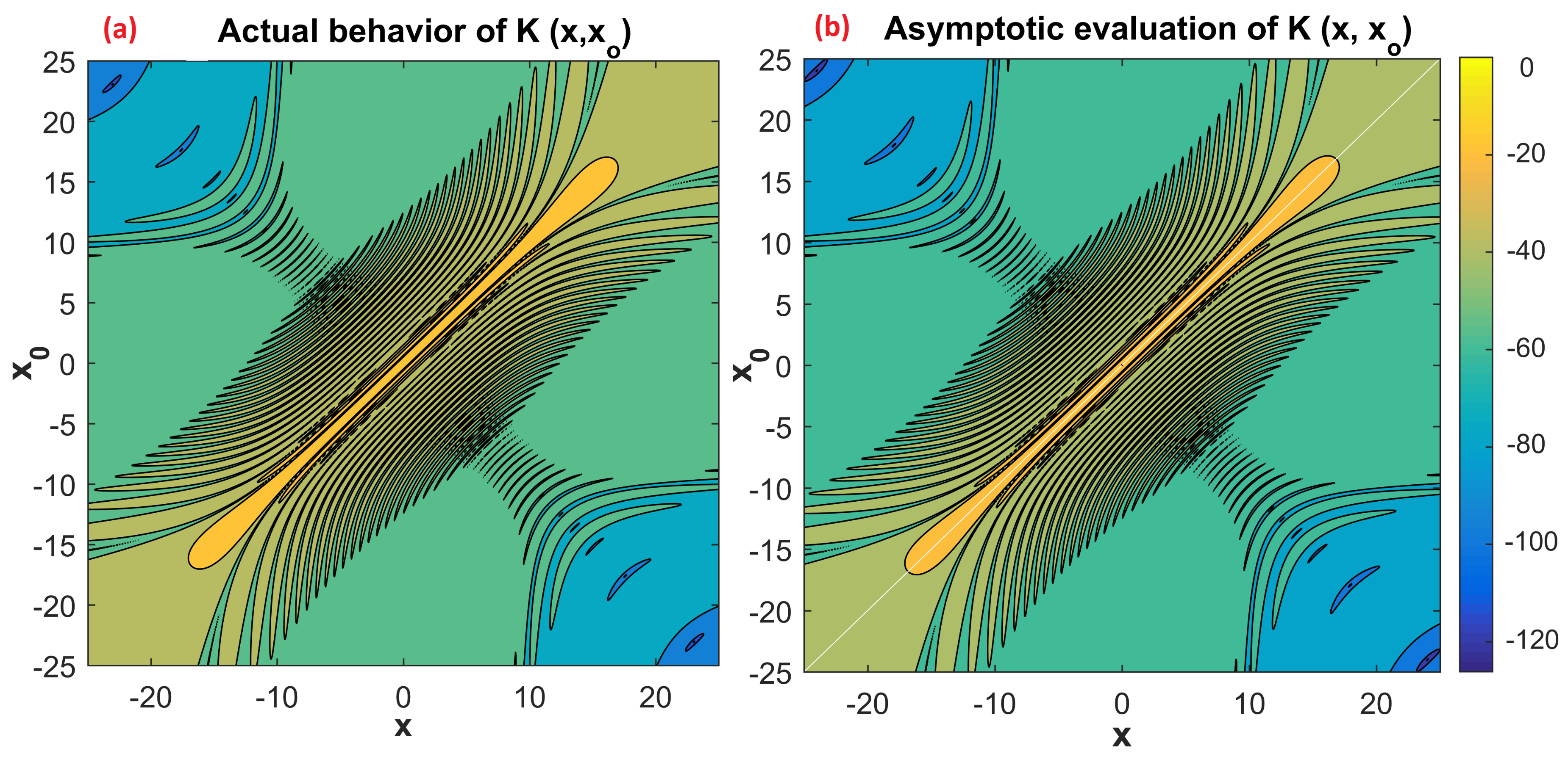
As said before, the asymptotic evaluation provided by (9) holds . The actual value of the kernel in can be obtained by particularizing (6) for , and by evaluating it. This turns out that
Anyway, the asymptotic evaluation (9) connects in a continuous way with the actual value of the kernel in .
In Figure 2 the actual behavior of , and the asymptotic evaluation (9) are sketched. The diagrams refer to a source with whose radiated electric field is observed along the axis . Note as, despite the asymptotic evaluation is an approximate version of the kernel , it works very well in practice.
The expression of provided by (9) highlights that the kernel of the operator is not of convolution type with respect to the variables . With the aim to recast it in a form more similar to a convolution kernel, let us rewrite (9) in the form
The last expression of suggests to introduce the following transformation
which allows expressing the operator in the form
where
The variable represents one of the two elliptical coordinates, and it is described in details in the Appendix A. By introducing the other elliptical coordinate , which is defined as
it results that . Consequently, the kernel can be rewritten as
At this stage, apart for the amplitude terms and , the kernel is more similar to a convolution kernel. With the aim to evaluate the possibility of approximating with a purely convolution kernel, let us expand the amplitude terms and in Laurent series. Since the point is a pole of order 1, the Laurent expansions of and have the following structure
where , and denote the terms of the Laurent expansion related to the positive powers of .
The possibility of truncating the expansions (17) to the first term is related to the extension of the region on which the couple of variables , changes. Consequently, the possibility of approximating the amplitude terms as
depends on the extension of the observation domain.
In the Appendix B, we discuss about the validity region of the approximation (18). Furthermore, we show that the value of changes with respect to the distance ; consequently, also the validity region of the approximation (18) changes in terms of .
From what said above, it follows that if then the approximation (18) works well, and the kernel can be approximated as a convolution kernel of sinc type given by
Differently, if , the approximation (18) does not work. In such case, the expression of provided by (16) cannot be approximated with a purely convolution kernel. However, in order to underline the differences with the sinc kernel (19), let us recast the expression of by substituting (17) in (16). By doing this, we obtain that
Naturally, for as said above, the second term in (20) is approximately constant and equal to ; instead, it is different from 0 outside.
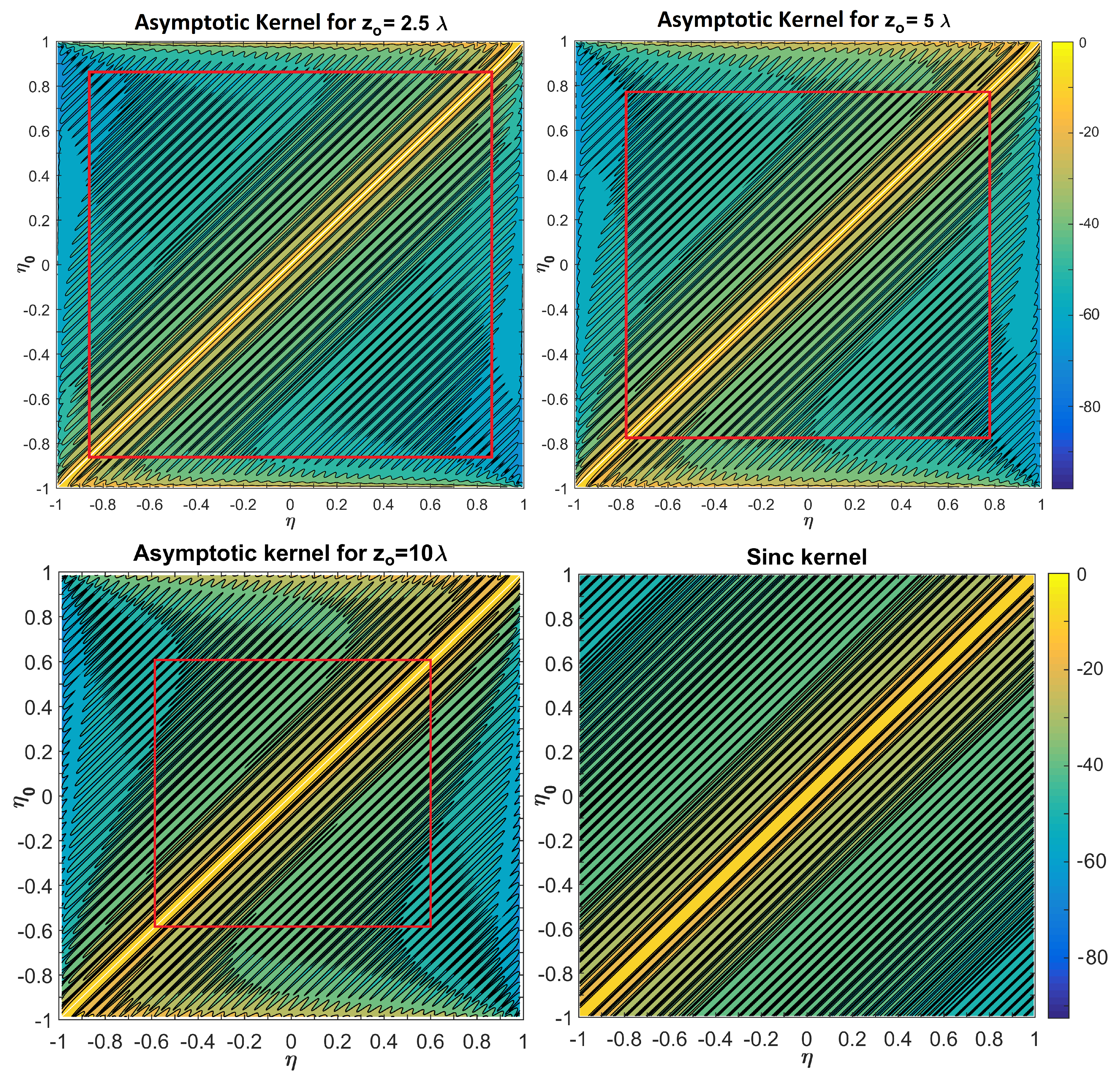
As in the figure, the asymptotic evaluation has the same behavior of the sinc kernel in the region which is highlighted by the square in red. Note that this region has a different extension in the cases , , and . that In the region outside, , the difference between the asymptotic kernel and the sinc kernel is due to the fact that the amplitude terms and are different to each other and not proportional to . Regarding the growth that the asymptotic kernel exhibits for , it is due to the terms that arises by passing from the variables to the variables .
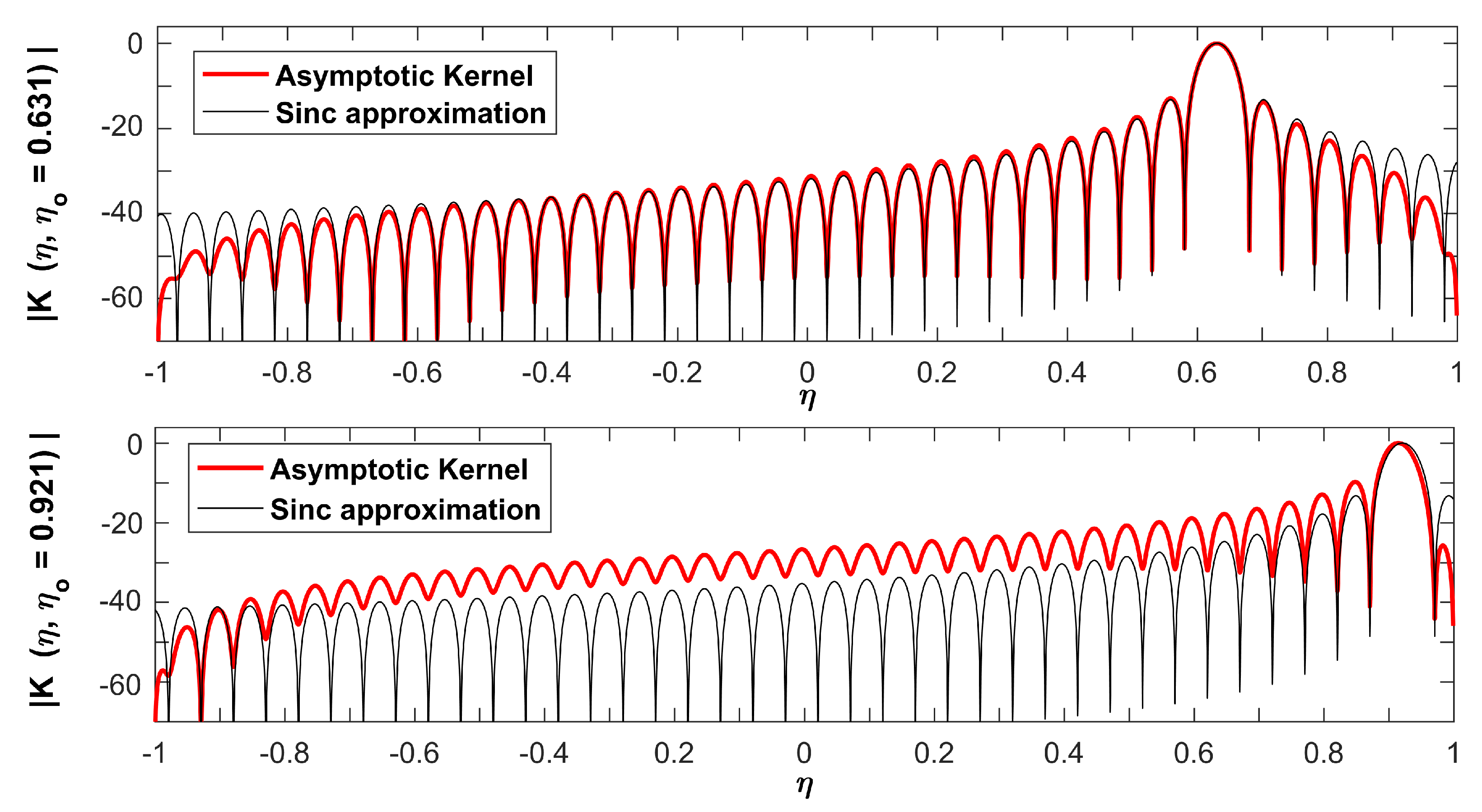
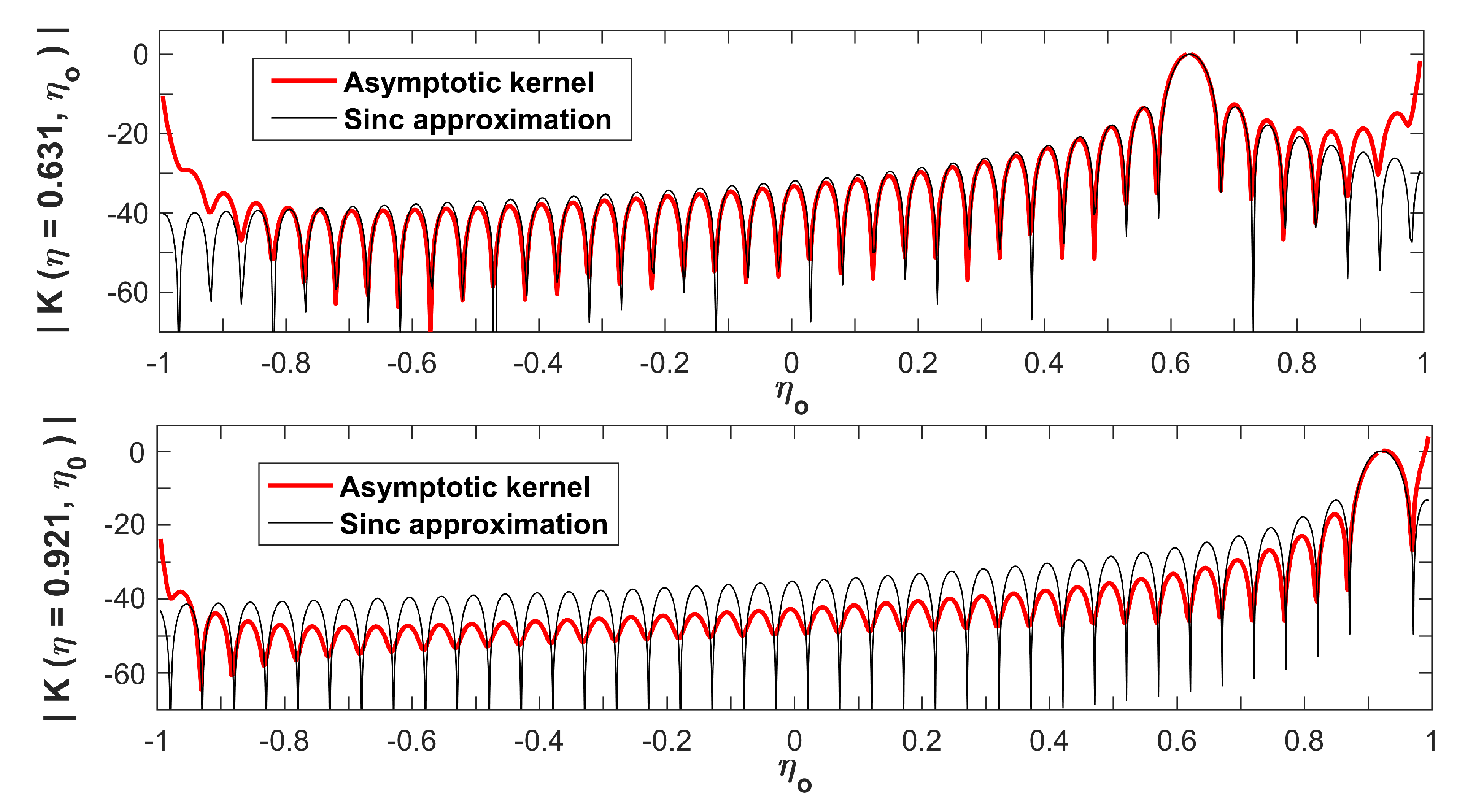
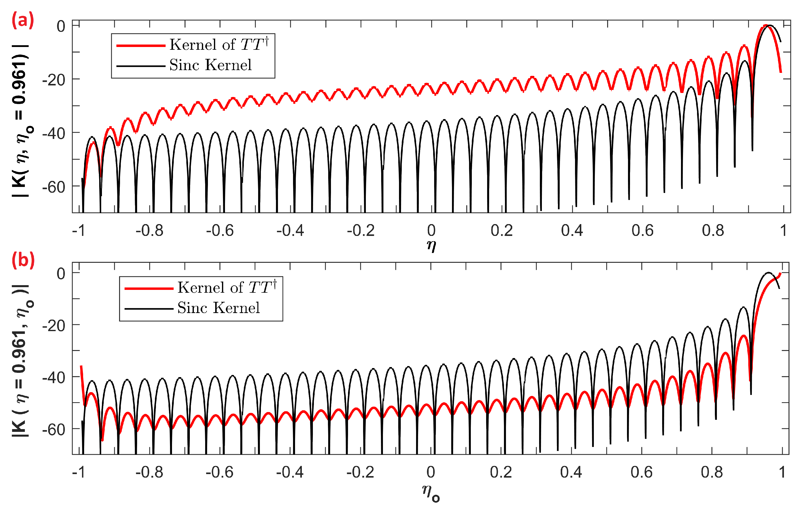
The aspects highlighted above can be observed also in the diagrams of the Figure 4 and Figure 5 which illustrate some cuts of the second graphs in Figure 3. In particular, Figure 4 shows the asymptotic evaluation, and the sinc kernel in terms of for two different values of . Instead, Figure 5 shows the asymptotic evaluation and the sinc kernel in terms of for two different values of .
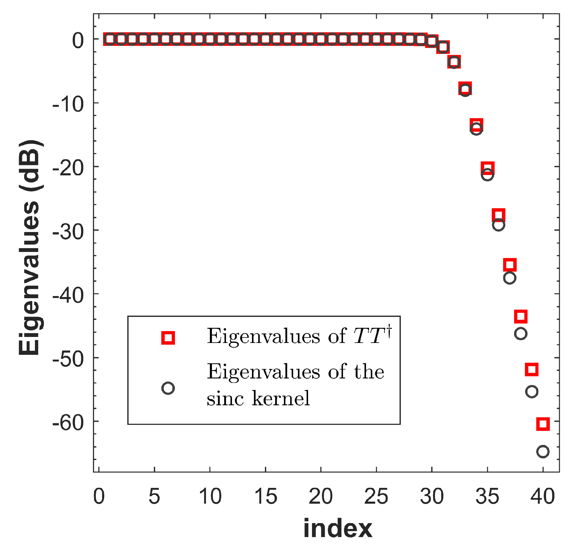
With reference to a configuration where the sinc approximation of the kernel holds, in Figure 6 the eigenvalues of the operator and those of the linear integral operator with the sinc kernel are compared. As can be seen from the figure, the eigenvalues of the operator with the sinc kernel overlaps with those of the operator . This fact is very important since the eigenspectrum of a linear integral operator with a sinc kernel is known in closed-form.
4. Sampling Scheme under the Sinc Approximation of the Kernel
With reference to the case where the sinc approximation works, in this section we show how to efficiently discretize the eigenvalue problem in order to obtain a discrete model that well approximate the mathematical properties of the continuous operator .
Under the assumption that , the considered eigenvalue problem can be explicitly written in the form
Hence, by fixing , the integral Equation (21) can be recast as
Since the integral operator involved in (22) is of the Slepian–Pollak type, the eigenspectrum of such an operator is known in closed-form and it is provided in the Appendix C. Here, instead, we focus on the discretization of the integral Equation (22). In particular, we show how to discretize such equation in order to obtain a discrete eigenvalue problem for a matrix whose eigenvalues are the same of the continuous problem, and whose eigenvectors contain the samples of the eigenfunctions .
The kernel of the integral Equation (22) is a band-limited function with respect to the variable whose band is . Hence, in order to discretize the eigenvalue problems (22), the sampling-theory approach developed in [25] can be applied. The latter provides the following linear system
where
- is the vector whose elements are the samples of collected with a step length equal or higher than the Nyquist step ( with ),
- is the matrix whose generic element is given by
In the Appendix C all the steps required to pass from the continous model (22) to the discrete model (23) are shown. The latter represents the eigenvalue problem for the matrix , and (apart for the truncation error of the sampling series (A6) and (A7)) it exhibits the same eigenvalues of the Fredholm integral Equation (21) and (22). Furthermore, since the -th eigenvector of ( ) contains the samples of collected with a sampling distance lower or equal than the Nyquist distance, the knowledge of allows recovering the correspondent eigenfunction , and consequently also .
It is interesting to note as the dimension of the matrix , and that of the vector depends on the oversampling factor . In fact, , and where is the number of samples collected with a sampling step that fall in the interval ; hence, . The latter if (or in other words if the sampling frequency is equal to the Nyquist frequency) is called the Shannon number, and it is exactly equal to the number of degrees of freedom N.
The value of the oversampling factor (or equivalently the value of the sampling frequency) affects also the level above which the eigenvalues of the continuous problem are well approximated by the eigenvalues of the matrix . In fact, a sampling frequency equal to the Nyquist frequency () allows approximating the eigenvalues before the knee, which corresponds the most significant part of the spectrum of the radiation operator . Instead, a sampling frequency a little bit higher than the Nyquist frequency (which correspond to set a little bit higher than 1) allows approximating also some of the eigenvalues beyond the knee. Hence, an increase of the oversampling factor bring a reduction of the level until which the eigenvalues of the continuous operator are well approximated by the eigenvalues of the matrix .
5. NDF and Sampling Strategy When the Kernel Is Not of Sinc Type
In this section, with reference to the case where the extension of the observation domain is wide enough that the sinc approximation (19) does not work, we discuss about
- How to compute the singular values behavior of the radiation operator ;
- How to discretize the eigenvalue problem in order obtain a discrete model that well approximates the eigenvalues .
As regards the first point, it results that the singular values of the radiation operator are given by the square root of the eigenvalues of but also by the square root of the eigenvalues of . Hence, if , in order to predict the singular values of the radiation operator it is possible to refer to the operator . As shown in [29], the kernel of is well approximated by a sinc function of difference type also if is significantly greater . Consequently, according to [31], the singular values of exhibit a step like behavior with the knee occurring at the index
also if . Hence, as regards the behavior of the singular values of , the results shown in the Appendix C for the case work also for .
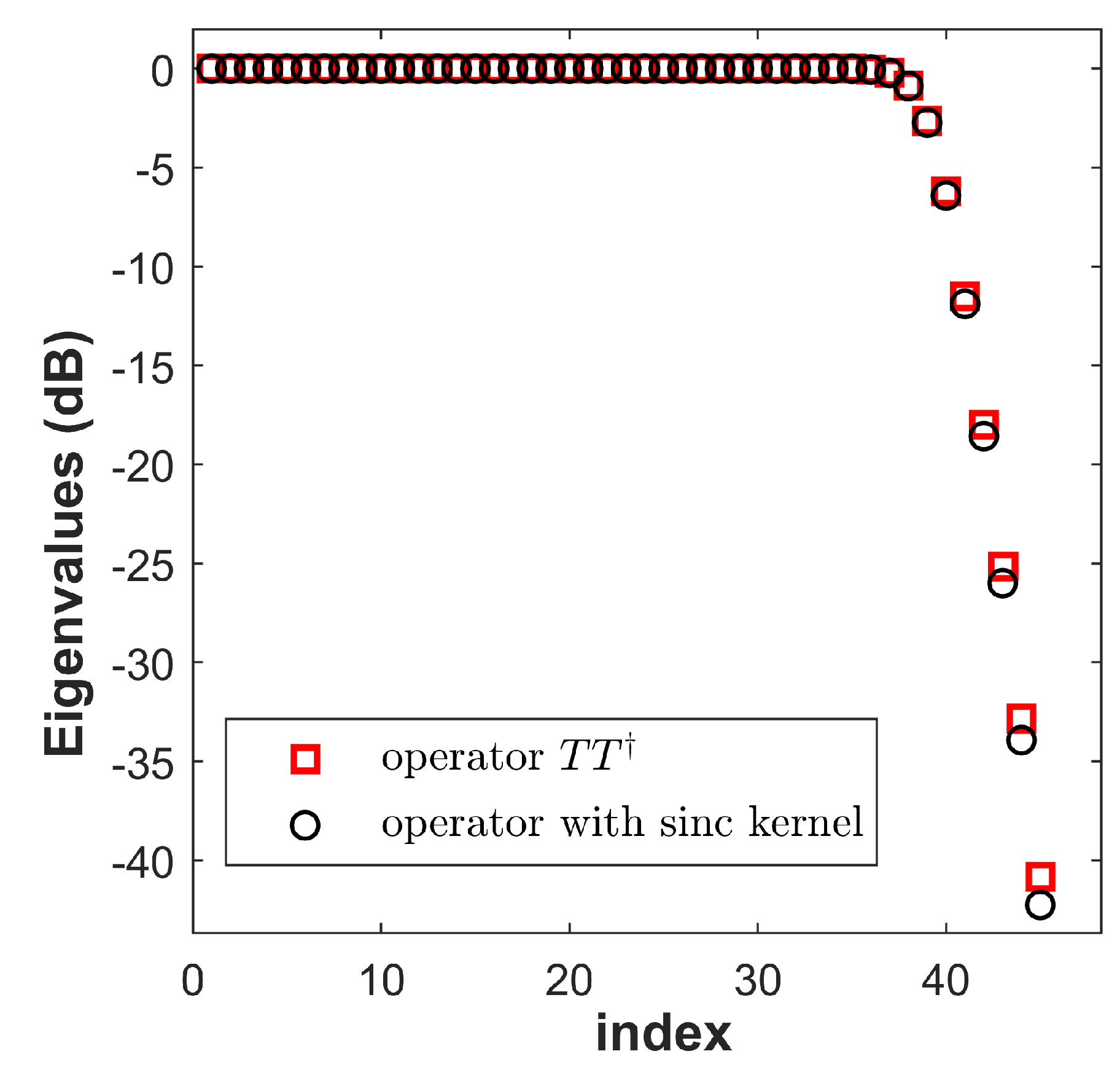
Note that as from the equality between the eigenvalues of and the eigenvalues of follows that despite for the kernel of is very different from the sinc kernel (19), the behavior of the eigenvalues of is well approximated by the eigenvalues of a linear integral operator with the sinc kernel (19). This can be understood by considering that the eigenvalues are given by . Since is an integral operator, the integral mitigates the difference between the actual kernel and the sinc kernel (19) making the eigenvalues of the two correspondent integral operators very similar. In order to corroborate what has just said said, in Figure 7 we compare the kernel of and the sinc kernel along the axis and , instead, in Figure 8 we show the eigenvalues of and those of the integral operator with the sinc kernel (19). Both the figures refer to the configuration , , .
It is interesting to note that despite the cuts of the two kernels overlap only in the region of the main lobe, the eigenvalues of the two operators are very similar.
At this point, let us discuss about how to discretize the eigenvalue problem in order to obtain a discrete problem for a matrix whose eigenvalues well approximate those of the continuous problem. In such case, since the kernel of the operator is not of convolution type, the sampling theory approach cannot be used. Hence, differently from the Section 4, the criterion exploited in the discretization is not based on the bandwidth of the kernel but on the reduction of the error between the eigenvalues of the continuous model and those of the discrete model.
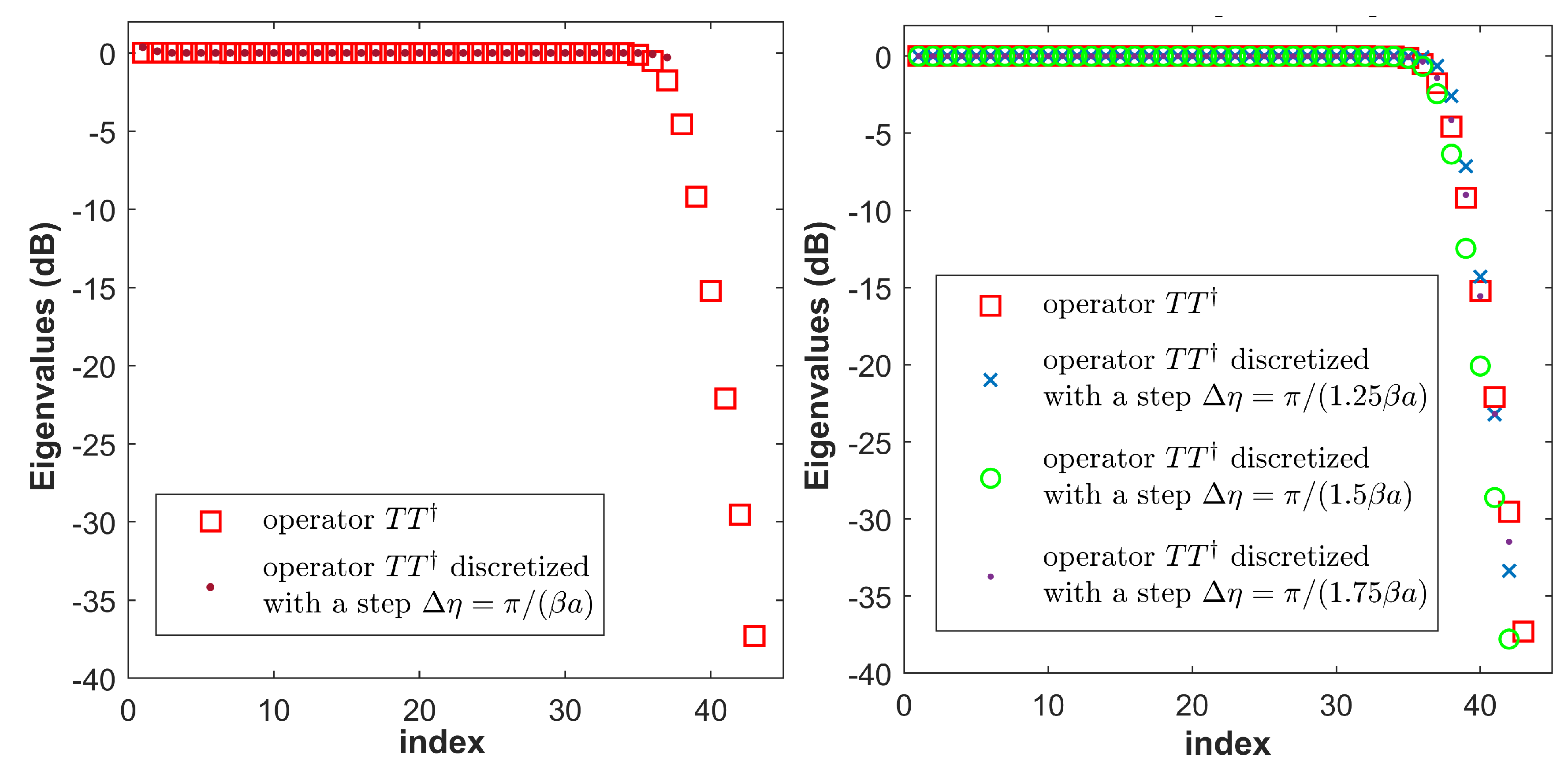
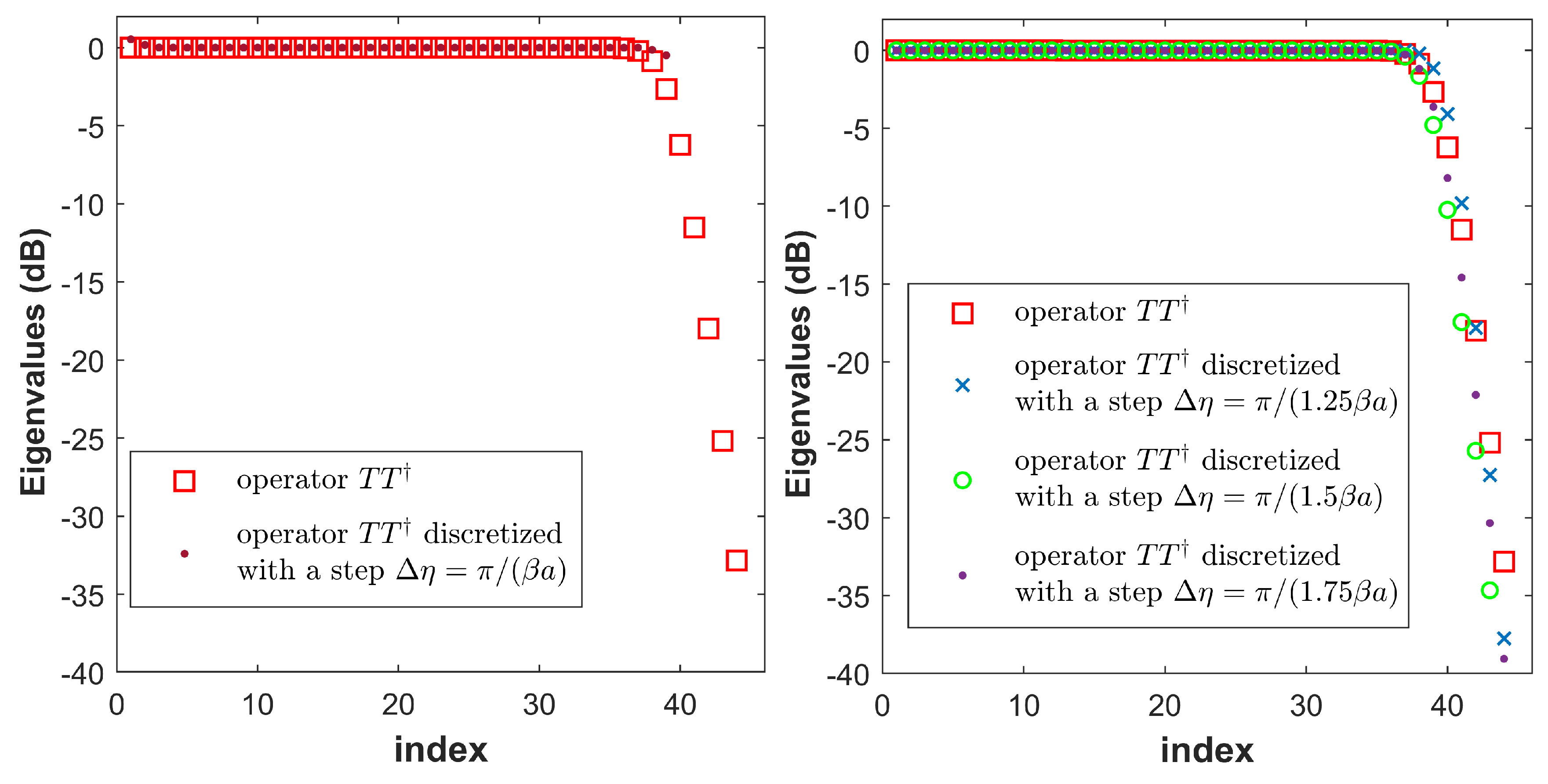
In order to give a guideline for the discretization of the integral equation , we perform some numerical simulations which differ each other for the extension of the observation domain , and/or for the sampling step . The results obtained by this numerical analysis are shown respectively in the Figure 9 and Figure 10 which illustrate the eigenvalues of , and those of the discrete operator obtained discretizing with a sampling step . In particular, Figure 9 refers to the configuration , , ; instead, Figure 10 refers to the configuration , , .
As can be seen from the figures, in both cases (, and ) a sampling step is already sufficient to approximate the relevant eigenvalues of the operator , and consequently, the relevant singular values of the radiation operator . Instead, in order to approximate the most significant eigenvalues beyond the knee, it is necessary a sampling step lower than which corresponds to an oversampling factor slightly higher than 1. Naturally, the value of the oversampling factor depends both on the level until which we want to approximate the eigenvalues of the continuous problem and on the desired accuracy.
Let us remark that despite the results obtained in this section can appear very similar to those shown in Section 4, there is a substantial difference. In Section 4, we provide the minimum sampling frequency that allows to well approximate both the eigenvalues and the eigenfunctions of the continuous model; here, instead, we limit our analysis to the approximation of the eigenvalues.
From the sampling in the variable to the sampling in the variable x
At this stage, the last thing to is to find the position of the samples in x domain starting from to the knowledge of the samples in domain. In order to do this, we must solve the equation
for each . By remembering Equation (12) and taking into account that , Equation (26) can be explicated as
where with .
Equation (27) represents an hyperbola whose foci are the points , and . Hence, when increases the point moves along such hyperbola. The latter can be rewritten in the form
From the last equation, it follows that the optimal location of the sampling points is given by
where denotes the integer nearest to . Note that if we choose the first sample in domain in , it results that . In such condition, and Equation (29) further simplifies.
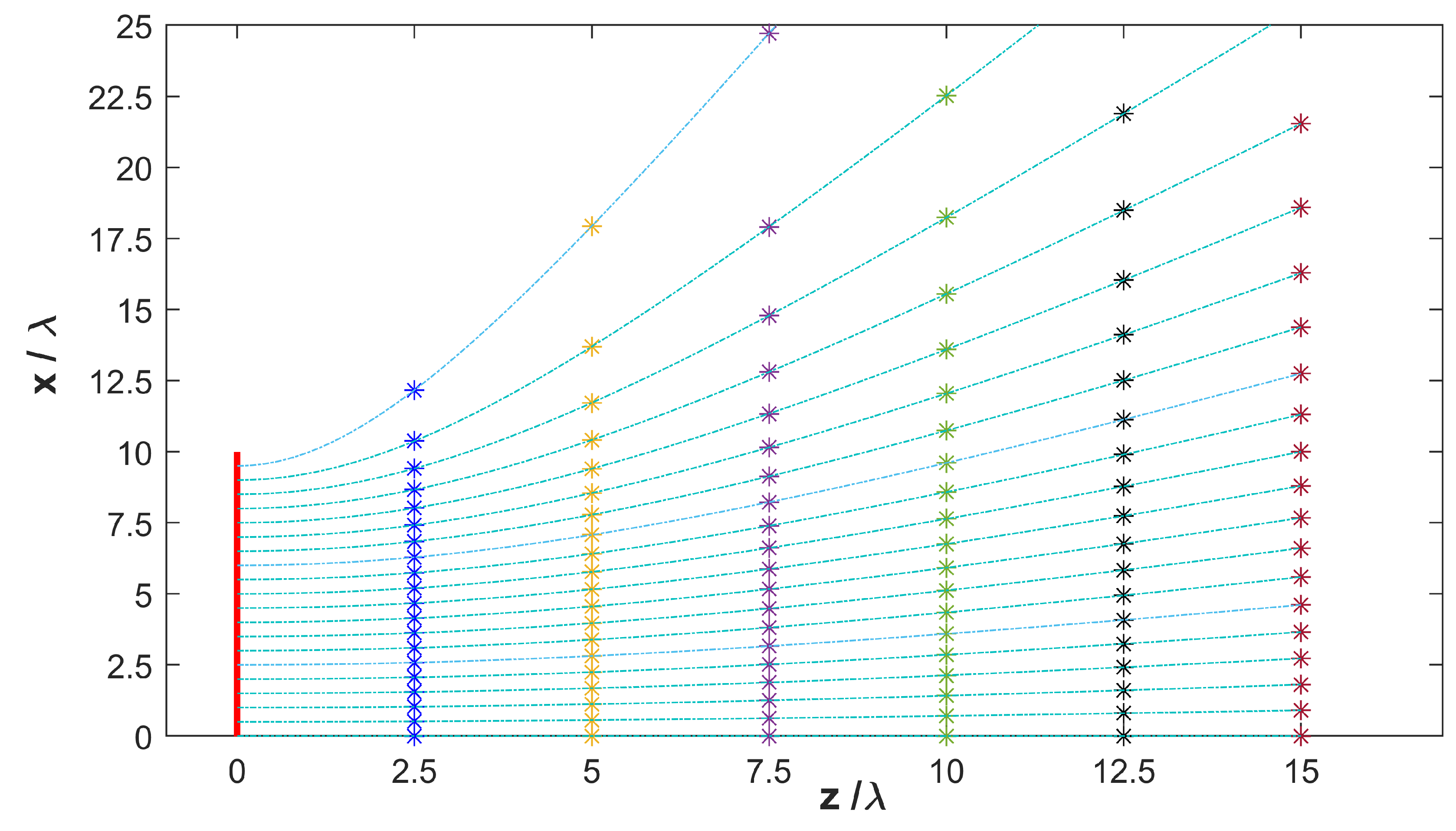
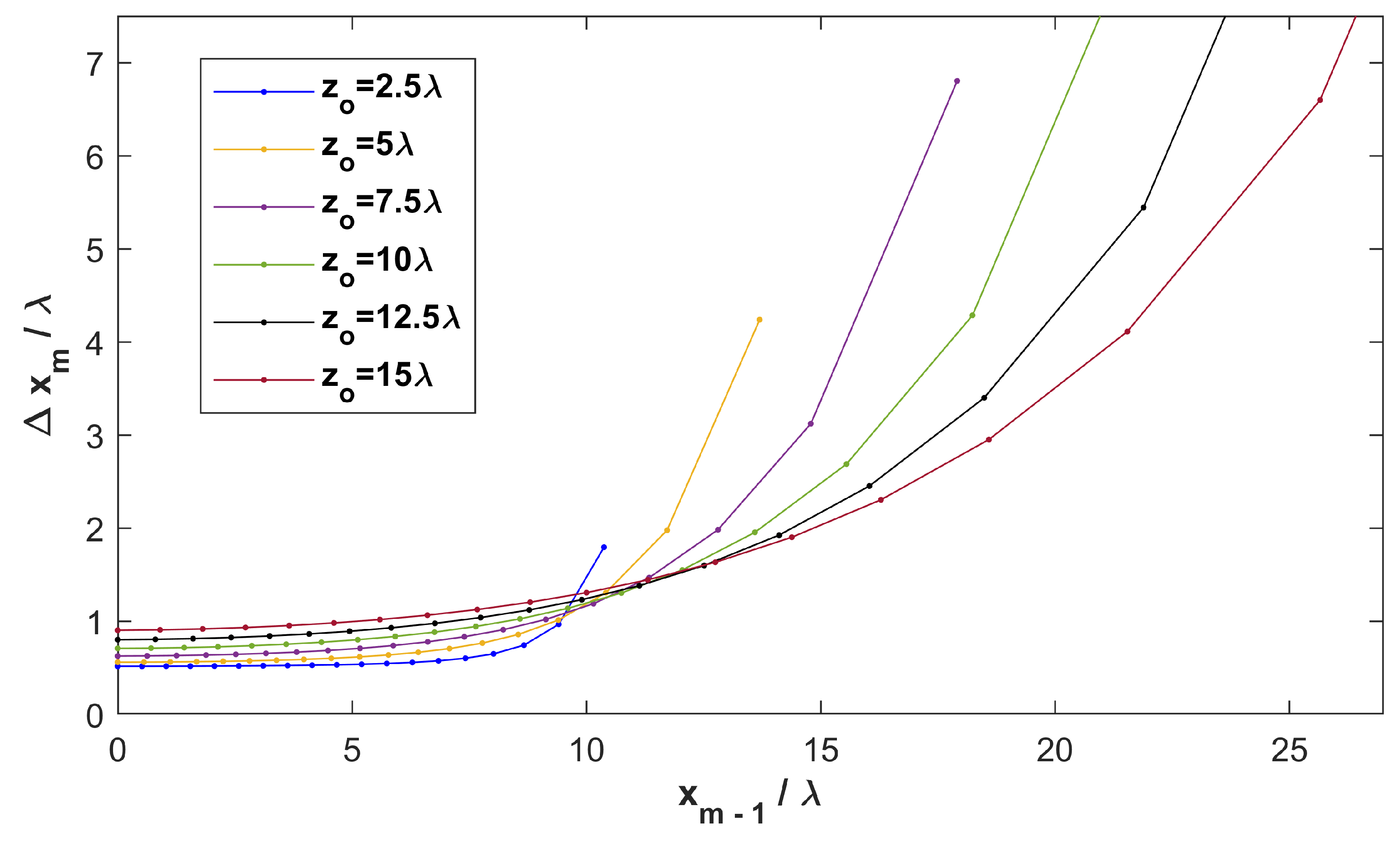
In Figure 11 the locations of the sampling points for different values of is shown, instead, in Figure 12 the behavior of the sampling step in terms of the variable is depicted.
The spacing of the sampling points shown in Figure 12 is well understood if we analyze the behavior of the transformation shown in Figure A1. For little of values of x the relation between and x is quasi-linear, hence, the uniform sampling step maps into a quasi uniform sampling step . Differently, when x increases, the relation between and x is non-linear; consequently, the uniform sampling step maps into a spatially varying sampling step . Furthermore, since when x increases a little variation of the variable produces a large of the variable x, it happens that the sampling step raises when x increases (see Figure 12). Summarizing, for small values of x (in the central region of the observation domain) the sampling step is quasi-uniform. Instead, when x moves toward the edges of the observation domain the sampling step is non-uniform, in particular, it increases gradually with the growth of x.
A last comment is related to the behavior of the sampling step in terms the distance . As can been seen from Figure 12, the sampling step is never less than , and it increases also when raises. Consequently, we can conclude the sampling step increases with respect to x, and .
6. Conclusions
In this paper a strategy to collect the radiated field in inverse source problem has been proposed. The basics idea of such sampling strategy is to find the optimal locations of the sampling points that allow to approximate the singular values behavior of the radiation operator as well as possible with a number of samples as low as possible. The study has been done with reference to a geometry where the electric field radiated by a strip of magnetic current is observed on a bounded line parallel to the source.
Since the kernel of the eigenvalue problem is neither convolution nor band-limited, the sampling theory approach could not be applied to find the optimal locations of the sampling points. For this reason, by exploiting an asymptotic approach and a suitable change of variables, we have recast the kernel of in the new variables . In such new variables, if the extension is lower than , the kernel of the eigenvalue problem can be approximated with a band-limited function of difference type; instead, if is greater than the kernel remains not of convolution type.
In the first case, the sampling theory approach can be applied. The latter turns out that a sampling step equal to the Nyquist step allows approximating all the part of the singular spectrum (singular values, and singular functions) corresponding to the singular values of before the knee. Instead, a sampling step slightly lower than the Nyquist step (which corresponds to a number of samples a little bit higher than the Shannon number) allows approximating also the part of the singular spectrum corresponding to the most relevant singular values beyond the knee.
Regarding the case , the sampling theory approach could not be applied. Hence, in such case we have performed a numerical analysis to establish the sampling step for which the discrete operator exhibits the same singular values of the radiation operator . From such a numerical analysis, we have found that also in this case a sampling step allows approximating the singular values before the knee. Instead, a sampling step with an oversampling factor slightly lower than 1 allows obtaining a discrete model that shares with the radiation operator not only the singular values before the knee but also the first singular values beyond the knee. Consequently, at least for the approximation of the most significant singular values of , we can state that a sampling step with slightly higher than 1 suffices to capture the most significant singular values of the radiation operator in both cases (, and ).
Furthermore, let us remark that this sampling strategy brings to a spatially varying sampling step in x variable. In particular, since the relation between and x is quasi-linear for x around 0 and non-linear elsewhere, the uniform sampling in variable is recast in a quasi-uniform sampling around (in the central part of the observation domain), and in a strong spatially varying sampling in regions at the edges of the observation domain.
Before concluding, it is interesting to highlight the effect of the noise on data. Since the kernel of the radiation operator is of the Hilbert–Schmidt class (i.e., since the kernel is a square integrable function), the radiation operator is compact. As a consequence, the inverse operator is not continuous, and the singular values tend to zero as their index increases. This entails that the part of the noise that projects onto the singular functions associated to low singular values is strongly amplified in the inversion process, and this could provide a meaningful solution. In order to overcome this drawback, a regularization scheme must be employed. With the regularization, we accept to represent the unknown function with a finite number of singular functions, and this entails a reduction of the resolution but an increasing of stability. A crucial role in the regularization is played by the number of singular components that must been considered. If the SNR is not so high (as it often happens) then one can at best stably reconstruct only the projection of the density current J onto the space spanned by the singular functions corresponding to the singular values before the knee. Hence, in this case, it sufficient to discretize the continuous model with a sampling step that allows approximating well only such part of the singular system. Conversely, if a high SNR is available, in order to represent the the density current, it is possible to use also the singular functions beyond the knee not corrupted by the noise. In this last case, it is necessary to well approximate also such part of the singular system. Consequently, in the discretization of the continuous model a sampling step is required.
Finally, it is worth noting that the approach developed in this paper can be extended also to more realistic scenario involving geometries.
Author Contributions
Conceptualization, R.P.; methodology, R.P. and R.M.; software, R.M.; validation, R.M.; formal analysis, R.P. and R.M; investigation, R.M.; resources, R.P.; data curation, R.M.; writing—original draft preparation, R.M.; writing—review and editing, R.M.; visualization, R.M.; supervision, R.P.; project administration, R.P.; funding acquisition, R.P. All authors have read and agreed to the published version of the manuscript.
Funding
This work was funded by the European Union and the Italian Ministry of University and Research funding through Programma Operativo Nazionale Ricerca e Innovazione 2019 / 2020-CUP .
Conflicts of Interest
The authors declare no conflict of interest.
Appendix A
In this appendix we provide some useful details about the non-linear transformation
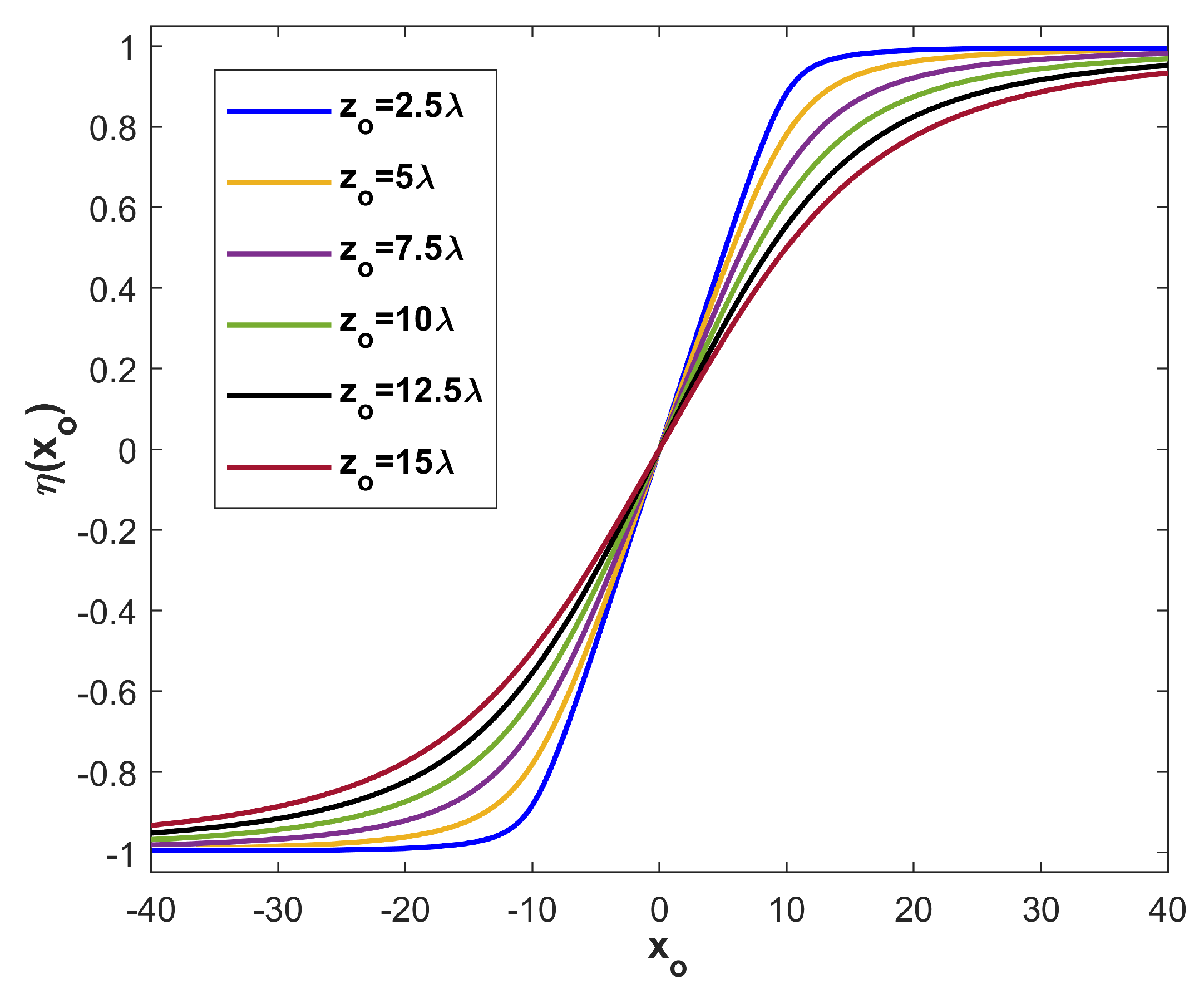
Such transformation realizes a warping of the variable . In particular, it stretches the set into . The multiplicative constant has been chosen in such a way that when , hence the possible values of the variable are limited to the set . Figure A1 shows the behavior of with respect to the variable for different values of the distance .
Figure A1.
Diagram of for different values of when .

As can be seen from the figure, exhibits a quasi-linear behavior for , and then it bends at the ends. In any case, the extension the linear behavior is bigger or equal than the source size a.
Since in this paper is bounded, transformation (A1) is invertible in the set . Hence, the inverse function exists, and it is given by
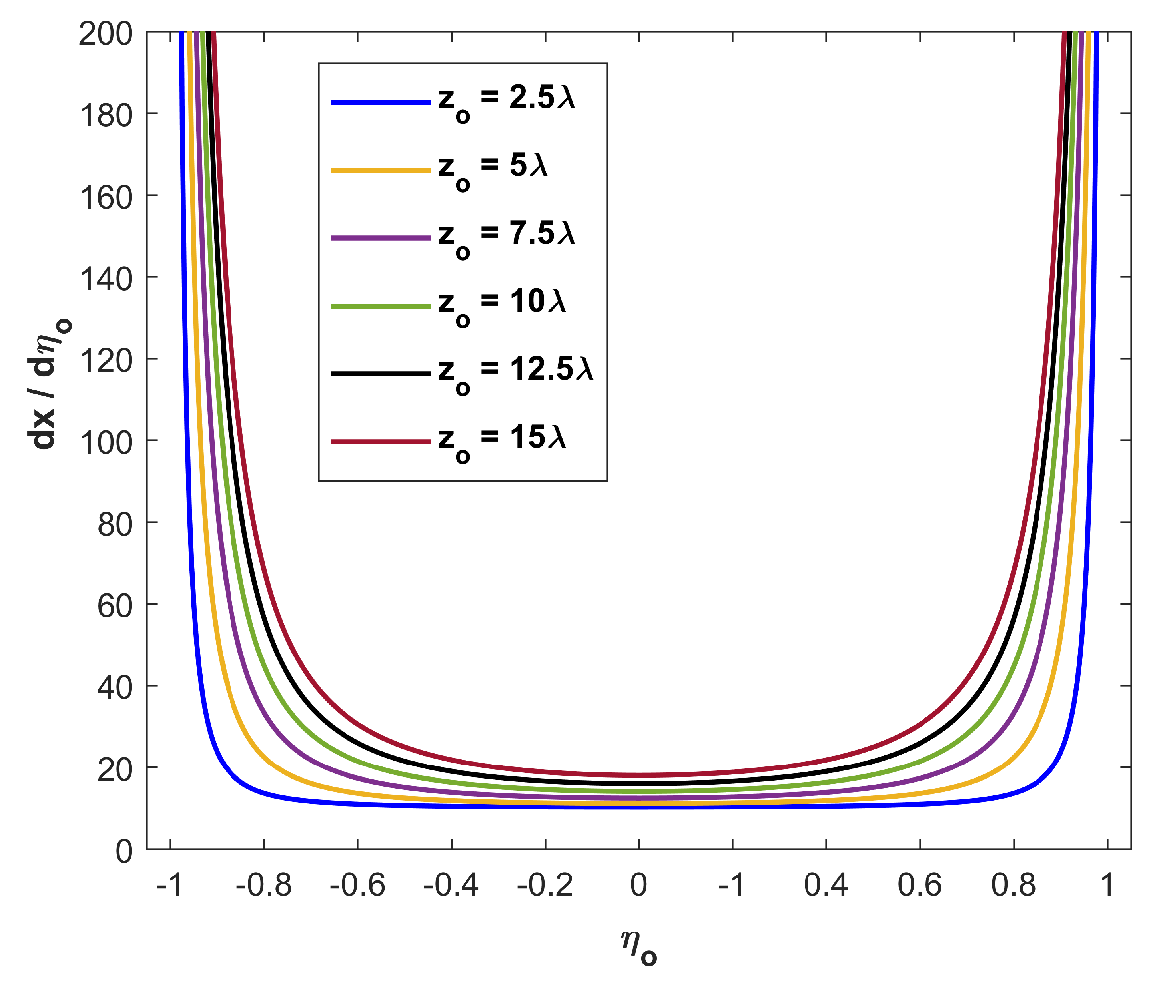
Finally, the first derivative of has the following expression
This term plays a crucial role, since it appears in expression of the asymptotic kernel when we pass from the variables to the variables . Figure A2 shows the behavior of in terms of for different values of .
Figure A2.
Diagram of in terms of for different values of . The picture refers to a source whose semi-extension a is equal to .
Figure A2.
Diagram of in terms of for different values of . The picture refers to a source whose semi-extension a is equal to .

Appendix B
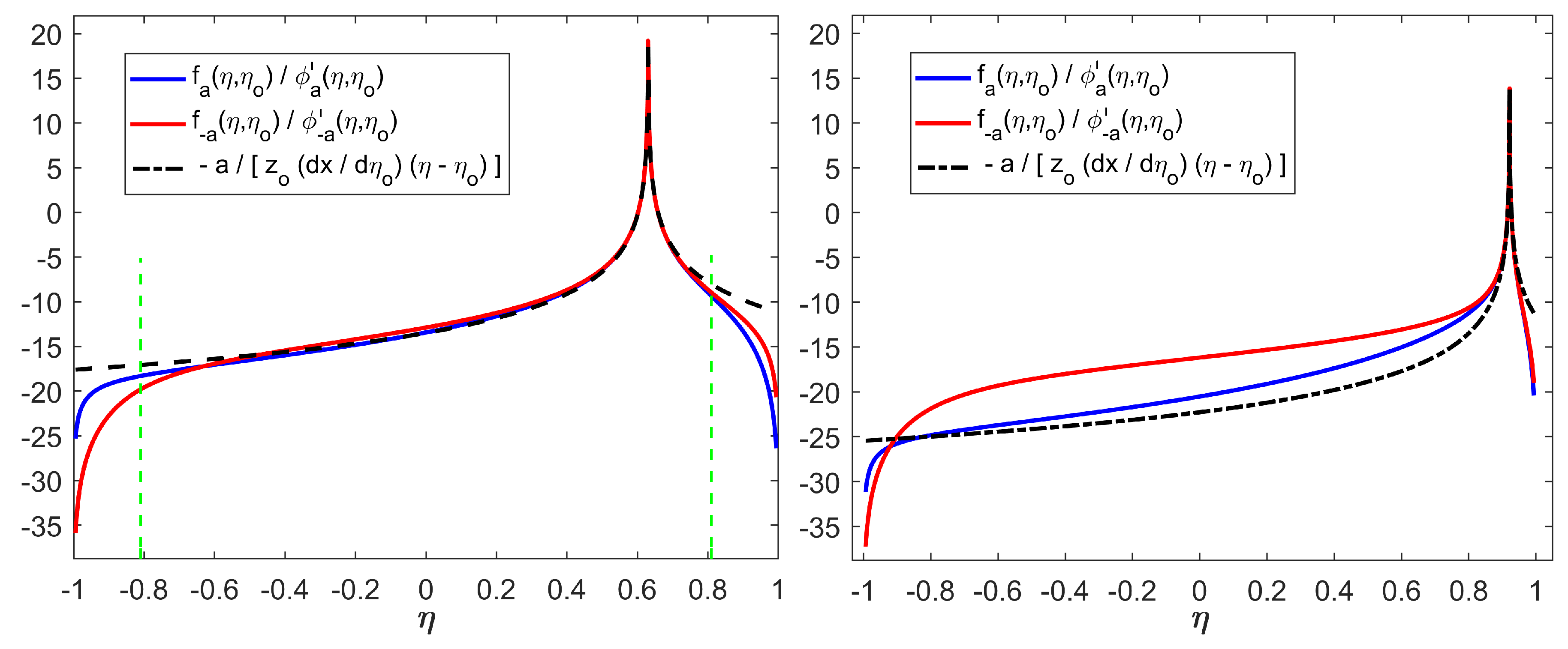
In this appendix we find the region of validity of the approximation (18). Naturally, such region is made up by all the points on which is significantly higher than the terms and . Since these functions depend on , also the extension of the region depends on .
Figure A3 shows the behavior of the functions , , and in terms of for two different values of . Note as the two cases are totally different. In the first example, since , approximation (18) works very well . In the second case, since , approximation (18) does not hold.
Figure A3.
Behavior of , , and in terms of for , and .

But, what is the value of ? In order to answer to this question, we have performed a numerical analysis. In such analysis, we have started by considering an observation domain with a little extension , and then we have gradually increased it until to reach the biggest value of for which the difference between the amplitude in dB of the asymptotic kernel and the amplitude in dB of the sinc kernel becomes lower than or higher than 3 in at least one point . Such particular value of has been denoted with , and the correspondent value in the domain has been denoted with . In other words, has been chosen as the minimum value between the maximum value of and the maximum value of for which the difference between the amplitude in dB of the asymptotic kernel and the amplitude in of the sinc kernel belong to the set in all the points . From such numerical analysis, we have obtained the results summarized in Table A1.

Table A1.
Values of , and for different values of the distance .
| 0.91 | ||
| 0.90 | ||
| 0.81 | ||
| 0.75 | ||
| a | 0.71 | |
| 0.66 | ||
| 0.65 | ||
| 0.63 | ||
| 0.63 | ||
| 0.63 |
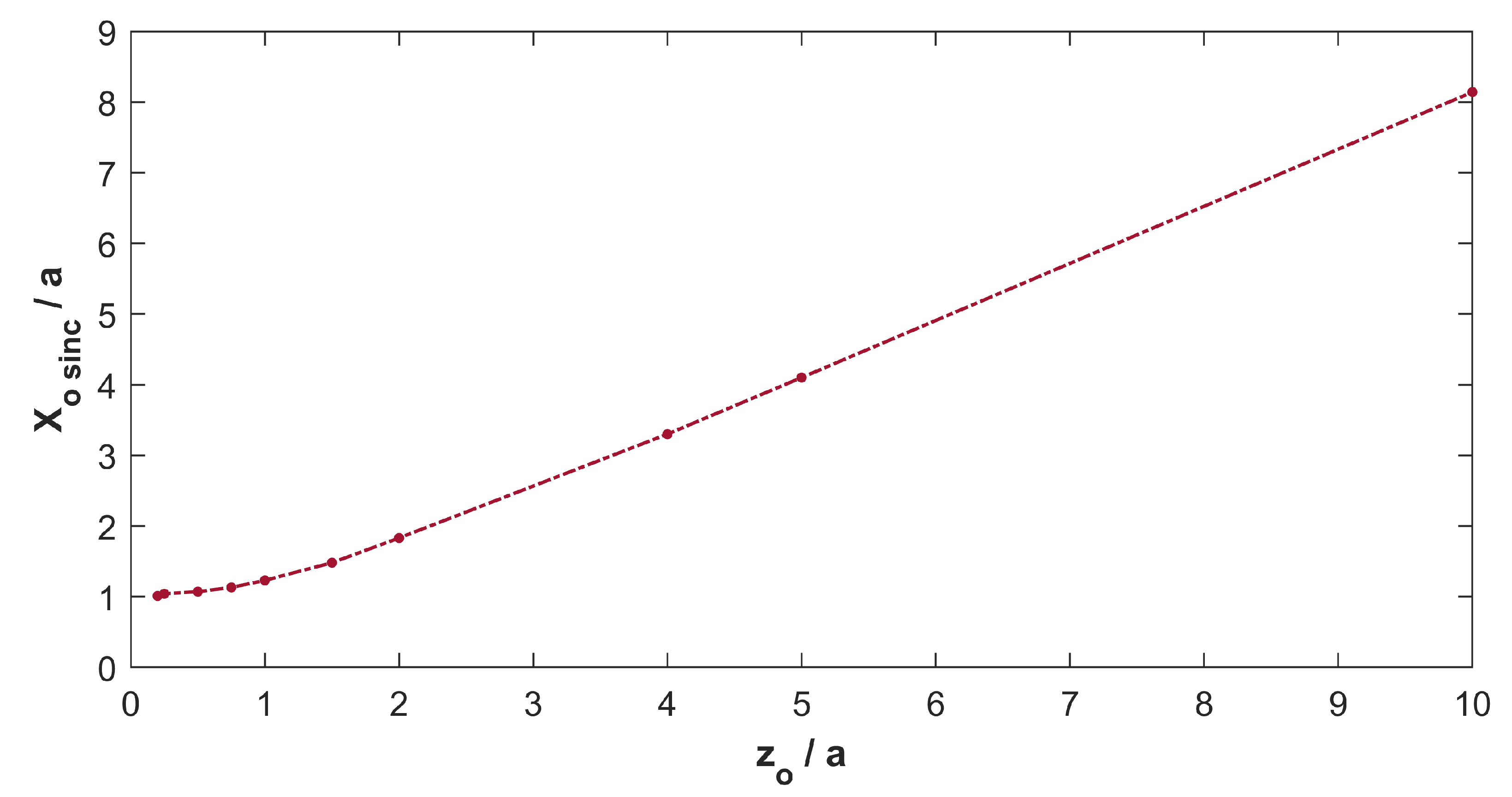
The table shows the values of for which the numerical analysis has been performed in the first column, the correspondent values of in the second column, and the correspondent values of in the third column. As can be seen from the table, for the value of decreases in such a way that remains almost unchanged. Instead, for the value of raises according to Equation (A2). In Figure A4 the behavior of with respect to is depicted.
Figure A4.
Diagram of in terms of .

Appendix C
In this appendix with reference to the cases in which the sinc approximation (19) works well, we provide the eigenspectrum of the linear integral operator , which (as explained in section II) is related to the singular values decomposition of the radiation operator .
Since the integral operator involved in (22) is of Slepian-Pollak type, the eigenspectrum of such operator is known in closed-form [31]. In particular, it results that the eigenvalues exhibit a step like with the knee occurring at the index
Furthermore, the eigenfunctions are related to the prolate spheroidal waves functions (PSWFs) , in fact, where is the so-called spatial bandwidth product, and are the eigenvalues of the Slepian-Pollak operator. Consequently, the eigenfunctions of the eigenvalues problem (21) are given by
As can be seen from Equation (A4), the number of relevant eigenvalues depends only on the geometric parameters of the configuration which are a, , and . Furthermore, such number differs from the case of unbounded observation domain only for the presence of the term ; in fact, in the case of unbounded observation domain the number of eigenvalues before the knee is given by [1]. This means that if is finite, the number of relevant eigenvalues reduces with respect to the case of unbounded observation domain of a factor .
Figure A1 depicted in the Appendix A, shows the behavior of with respect to for different values of the distance . As can be seen from figure, fixing the value of decreases when the distance increases. Consequently, if the value of remains unchanged, the number of relevant eigenvalues N is more similar to the when the distance between the observation domain and the source is low. Differently, if we want that the number of relevant singular values N remains unchanged when raises, then the extension of the observation domain has to raise according to Equation (A2) in the Appendix A.
Appendix D
In this appendix we show all the mathematical steps required to obtain the discrete eigenvalue problem (23) starting from the continuous model (22). Since the kernel of the integral Equation (22) is a band-limited function with respect to the variable , it can be sampled without loss of information with a sampling step equal or lower than the Nyquist distance (i.e., ). Consequently, the kernel can be represented through the Shannon sampling series
where with denoting an eventually oversampling factor, hence . The same expansion can be performed also for the eigenfunctions , hence, it results that
It is interesting to note that in general the Shannon sampling series of a band-limited function is made up by an infinite number of terms. However, since the variable , in such case the series (A6) and (A7) include only a finite number of terms given by the number of points which fall in the set .
Consequently, it results that
. The previous set of equations represents a linear system, hence, it can be written in the form .
References
- Solimene, R.; Maisto, M.A.; Pierri, R. Inverse source in the near field: The case of a strip current. J. Opt. Soc. Am. A 2018, 35, 755–763. [Google Scholar] [CrossRef] [PubMed]
- Mauermayer, R.A.M.; Weitsch, Y.; Eibert, T.F. Electromagnetic Field Synthesis by Hierarchical Plane Wave-Based Field Transformation. IEEE Trans. Antennas Propag. 2015, 63, 5561–5572. [Google Scholar] [CrossRef]
- Oliveri, G.; Rocca, P.; Massa, A. Reliable diagnosis of large linear arrays—A Bayesian compressive sensing approach. IEEE Trans. Antennas Propag. 2012, 60, 4627–4636. [Google Scholar]
- Eltayeb, M.E.; Al-Naffouri, T.Y.; Heath, R.W. Compressive Sensing for Millimeter Wave Antenna Array Diagnosis. IEEE Trans. Commun. 2018, 66, 2708–2721. [Google Scholar]
- Marengo, E.A.; Devaney, A.J. The inverse source problem of electromagnetics: Linear inversion formulation and minimum energy solution. IEEE Trans. Antennas Propag. 1999, 47, 410–412. [Google Scholar]
- Maisto, M.A.; Moretta, R.; Solimene, R.; Pierri, R. Phaseless arrays diagnostic by Phaselift in near zone: numerical experiments. In Proceedings of the 2017 Progress in Electromagnetics Research Symposium (PIERS), St. Petersburg, Russia, 22–25 May 2017. [Google Scholar]
- Schnattinger, G.; Eibert, T.F. Solution to the Full Vectorial 3-D Inverse Source Problem by Multilevel Fast Multipole Method Inspired Hierarchical Disaggregation. IEEE Trans. Antennas Propag. 2012, 60, 3325–3335. [Google Scholar] [CrossRef]
- Bertero, M.; Boccacci, P. Introduction to Inverse Problems in Imaging; IOP Publishing: Bristol, UK, 1998. [Google Scholar]
- Pierri, R.; Soldovieri, F. On the information content of the radiated fields in the near zone over bounded domains. Inverse Probl. 1998, 14, 321–337. [Google Scholar] [CrossRef]
- Leone, G.; Maisto, M.A.; Pierri, R. Inverse Source of Circumference Geometries: SVD Investigation Based on Fourier Analysis. Progr. Electromagn. Res. M 2018, 76, 217–230. [Google Scholar] [CrossRef] [Green Version]
- Giordanengo, G.; Righero, M.; Vipiana, F.; Vecchi, G.; Sabbadini, M. Fast Antenna Testing With Reduced Near Field Sampling. IEEE Trans. Antennas Propag. 2014, 62, 2501–2513. [Google Scholar] [CrossRef]
- Solimene, R.; Maisto, M.A.; Pierri, R. On the singular spectrum of the radiation operator for multiple and extended observation domains. Int. J. Antennas Propag. 2013. [Google Scholar]
- Bucci, O.M.; Gennarelli, C.; Savarese, C. Representation of electromagnetic fields over arbitrary surfaces by a finite and nonredundant number of samples. IEEE Trans. Antennas Propag. 1998, 46, 351–359. [Google Scholar] [CrossRef]
- Solimene, R.; Maisto, M.A.; Pierri, R. Sampling approach for singular system computation of a radiation operator. J. Opt. Soc. Am. A 2019, 36, 353–361. [Google Scholar]
- Maisto, M.A.; Solimene, R.; Pierri, R. Optimal choice of measurement points in near field: Numerical results. In Proceedings of the 2018 IEEE International Symposium on Antennas and Propagation USNC/URSI National Radio Science Meeting, Boston, MA, USA, 8–13 July 2018. [Google Scholar]
- Maisto, M.A.; Solimene, R.; Pierri, R. Minimum measurement points in near field: Numerical results. In Proceedings of the 2018 Progress in Electromagnetics Research Symposium (PIERS), Toyama, Japan, 1–4 August 2018. [Google Scholar]
- Migliore, M.D. Near field antenna measurement sampling strategies: From linear to nonlinear interpolation. Electronics 2018, 7, 257. [Google Scholar] [CrossRef] [Green Version]
- Di Francia, G.T. Degrees of freedom of an image. J. Opt. Soc. Am. A 1969, 59, 799–804. [Google Scholar] [CrossRef] [PubMed]
- Piestun, R.; Miller, D.A. Electromagnetic degrees of freedom of an optical system. J. Opt. Soc. Am. A 2000, 17, 892–902. [Google Scholar] [CrossRef]
- Miller, D.A. Communicating with waves between volumes: evaluating orthogonal spatial channels and limits on coupling strengths. Appl. Opt. 2000, 39, 1681–1699. [Google Scholar] [CrossRef] [Green Version]
- Newsam, G.; Barakat, R. Essential dimension as a well-defined number of degrees of freedom of finite-convolution operators appearing in optics. J. Opt. Soc. Am. A 1985, 2, 2040–2045. [Google Scholar] [CrossRef]
- Isernia, T.; Leone, G.; Pierri, R. Sulle dimensioni “essenziali” dei campi: Un approccio ai valori singolari. In Proceedings of the IX Riunione Naziale di Elettromagnetismo, Assisi, Italy, 5–8 October 1992. [Google Scholar]
- Somaraju, R.; Trumpf, J. Degrees of freedom of a communication channel: Using DOF singular values. IEEE Trans. Inf. Theory 2010, 56, 1560–1573. [Google Scholar] [CrossRef]
- Khare, K.; George, N. Sampling theory approach to prolate spheroidal wave-functions. J. Phys. A Math. Gen. 2003, 36, 10011–10021. [Google Scholar] [CrossRef]
- Khare, K.; George, N. Sampling-theory approach to eigenwavefronts of imaging systems. J. Opt. Soc. Am. A 2005, 22, 434–438. [Google Scholar]
- Khare, K. Sampling theorem, bandlimited integral kernels and inverse problems. Inverse Probl. 2007, 23, 1395–1416. [Google Scholar] [CrossRef]
- Leone, G.; Munno, F.; Pierri, R. Radiation Properties of Conformal Antennas: The Elliptical Source. Electronics 2019, 8, 531. [Google Scholar] [CrossRef] [Green Version]
- Solimene, R.; Maisto, M.A.; Pierri, R. Information Content in Inverse Source with Symmetry and Support Priors. Prog. Electromagn. Res. 2018, 80, 39–54. [Google Scholar] [CrossRef] [Green Version]
- Maisto, M.A.; Solimene, R.; Pierri, R. Resolution limits in inverse source problem for strip currents not in Fresnel zone. J. Opt. Soc. Am. A 2019, 36, 826–833. [Google Scholar] [CrossRef]
- Bleistein, N.; Handelsman, R. A. Asymptotic Expansions of Integrals; Dover Publications: New York, NY, USA, 1986. [Google Scholar]
- Slepian, D.; Pollack, H.O. Prolate spheroidal wave functions, Fourier analysis, and uncertainty—I. Bell Syst. Tech. J. 1961, 40, 43–63. [Google Scholar] [CrossRef]
Figure 1.
Configuration of the problem. The source domain (SD) is sketched in red, the observation domain (OD) in green.
Figure 1.
Configuration of the problem. The source domain (SD) is sketched in red, the observation domain (OD) in green.

Figure 2.
(a) Actual behavior of obtained by computing the integral (6) numerically. (b) Behavior of provided by the asymptotic evaluation. Both the diagrams are sketched in dB.
Figure 2.
(a) Actual behavior of obtained by computing the integral (6) numerically. (b) Behavior of provided by the asymptotic evaluation. Both the diagrams are sketched in dB.

Figure 3.
Amplitude of provided by the asymptotic evaluation for , and amplitude of the sinc kernel. The diagrams are shown in dB, and they refer to a source with .
Figure 3.
Amplitude of provided by the asymptotic evaluation for , and amplitude of the sinc kernel. The diagrams are shown in dB, and they refer to a source with .

Figure 4.
Behavior of in dB for () and (). The diagrams refer to the configuration (), and .

Figure 5.
Behavior of in dB for () and (). The diagrams refer to the configuration (), .

Figure 6.
Comparison between the eigenvalues of and those of the integral operator with the sinc kernel (19). The figure refers to the case , , .
Figure 6.
Comparison between the eigenvalues of and those of the integral operator with the sinc kernel (19). The figure refers to the case , , .

Figure 7.
(a) Kernel of in terms of for , and sinc kernel in terms of for . (b) Kernel of in terms of for , and sinc kernel in terms of for . The diagrams are in dB, and they refer to the configuration , , ().
Figure 7.
(a) Kernel of in terms of for , and sinc kernel in terms of for . (b) Kernel of in terms of for , and sinc kernel in terms of for . The diagrams are in dB, and they refer to the configuration , , ().

Figure 8.
Eigenvalues of the operator , and eigenvalues of the sinc kernel. The diagrams refer to the configuration , , ().
Figure 8.
Eigenvalues of the operator , and eigenvalues of the sinc kernel. The diagrams refer to the configuration , , ().

Figure 9.
Eigenvalues of the operator and those of its discrete version for different values of the sampling step . The diagrams refer to the configuration , , ().
Figure 9.
Eigenvalues of the operator and those of its discrete version for different values of the sampling step . The diagrams refer to the configuration , , ().

Figure 10.
Eigenvalues of the operator . The diagrams refer to the configuration , , ().

Figure 11.
Position of the sampling points for different values of when .

Figure 12.
Diagram of in terms of for different values of in the case .

© 2020 by the authors. Licensee MDPI, Basel, Switzerland. This article is an open access article distributed under the terms and conditions of the Creative Commons Attribution (CC BY) license (http://creativecommons.org/licenses/by/4.0/).
Share and Cite
MDPI and ACS Style
Pierri, R.; Moretta, R. Asymptotic Study of the Radiation Operator for the Strip Current in Near Zone. Electronics 2020, 9, 911. https://doi.org/10.3390/electronics9060911
AMA Style
Pierri R, Moretta R. Asymptotic Study of the Radiation Operator for the Strip Current in Near Zone. Electronics. 2020; 9(6):911. https://doi.org/10.3390/electronics9060911
Chicago/Turabian StylePierri, Rocco, and Raffaele Moretta. 2020. "Asymptotic Study of the Radiation Operator for the Strip Current in Near Zone" Electronics 9, no. 6: 911. https://doi.org/10.3390/electronics9060911
Note that from the first issue of 2016, this journal uses article numbers instead of page numbers. See further details here.