Rapid Reconstruction of Simulated and Experimental Temperature Fields Based on Proper Orthogonal Decomposition


1
School of Energy, Power and Mechanical Engineering, North China Electric Power University, Beijing 102206, China
2
School of Control and Computer Engineering, North China Electric Power University, Beijing 102206, China
3
China Datang Northwest Electric Power Test and Research Institute, Xi’an 710065, China
*
Author to whom correspondence should be addressed.
Appl. Sci. 2020, 10(11), 3729; https://doi.org/10.3390/app10113729
Submission received: 17 March 2020
/
Revised: 21 May 2020
/
Accepted: 26 May 2020
/
Published: 28 May 2020
(This article belongs to the Section Applied Industrial Technologies)
Abstract
:Temperature information has a certain significance in thermal energy systems, especially in gas combustion systems. Generally, measurements and numerical calculations are used to acquire temperature information, but both of these approaches have their limitations. Constrained by cost and conditions, measurement methods are difficult to use to reconstruct the temperature field. Numerical methods are able to estimate the temperature field; however, the calculation process in numerical methods is very complex, so these methods cannot be used in real time. For the purpose of solving these problems, a two-dimensional temperature field reconstruction method based on the proper orthogonal decomposition (POD) algorithm is proposed in this study. In the proposed method, the temperature field reconstruction task is transformed into an optimization problem. Theoretical analysis and simulations show that the proposed method is feasible. Gas combustion experiments were also performed to validate this method. Results indicate that the proposed method can yield a reliable reconstruction solution and can be applied to real-time applications.
1. Introduction
In gas combustion systems, temperature information not only shows details about the burning process, but also reveals the equipment running status. It has significant meaning for system safety and efficiency. There are numerous methods for measuring temperature. For example, conventional temperature measuring equipment, such as thermal resistances and thermocouples, are widely used in the combustion process. These instruments are convenient and efficient, but they can only be used for single-point measurements. It is impossible to install enough equipment for detailed information [1]. New temperature measurement techniques [2,3,4], such as acoustic measurement and optical measurement, can be used to reconstruct the temperature field. Although these techniques have been used in some combustion systems, many problems remain that may limit their application. For example, noise, vibration, and ash in the industrial environment may have a great impact on their accuracy. Furthermore, sensors involved in these techniques are difficult to install, and the measurement systems are complicated and expensive. All of these factors increase the difficulty of applying these techniques.
Numerical methods can also be used to acquire temperature information. For example, computational fluid dynamics (CFD) methods are employed to get accurate and detailed temperature information. However, numerical computations always involve a large amount of data, so they are exceptionally time-consuming and not suitable for real-time applications.
As mentioned above, in real applications, directly using a mass of empirical data or calculating data are difficult. How to make a use of these data has been a hot area of research in recent years. By using multi-resolution techniques and studying the hidden structure [5] of these data, the fractal-wavelet analysis [6,7,8] method can analyze and utilize the most essential characteristics of these data. As the fractal-wavelet analysis is convenient and efficient, it is used in many fields, such as image coding, texture discrimination, fractal analysis [8], distribution calculation [9], and antenna geometry analysis [10,11].
In order to solve the temperature measurement problem, inspired by the fractal-wavelet analysis method, the aim of this study is to develop a two-dimensional temperature field reconstruction method that can be used in real applications.
Some data reduction methods offer a new approach for solving these problems. These kinds of methods can derive a dimension reduction model with minimal information loss, which makes it possible to use CFD calculation data in real-time measurement. Among such methods, proper orthogonal decomposition (POD) is the most commonly used approach [12].
POD is an effective way to reduce data size—it is also known as Karhunen–Loève (KL) expansion or principal components analysis (PCA). It was first discussed by Pearson in 1901 [13]. Since then, POD has been used in many different domains, including signal analysis [14], data compression [15], image processing [16,17], chemical reaction analysis [18], and control systems [19,20]. The POD method was first introduced in fluid mechanics by Lumley [21]. Since then, it has been widely used in flow field analysis [22,23]. Allery used it to investigate particle dispersion [24], and Qin and Sun used it in flow field reconstruction [25,26]. The method has also been used in oceanography [27] and aerodynamics studies [28,29]. Furthermore, some researchers have developed optimization algorithms for sensor placement based on the POD method [27,30,31]. There are also some important studies on POD’s theoretical basis; for example, Kirby gave detailed discussions on the POD method [12], and Lu et al. presented a review of the POD method in a variety of research areas [32].
In this study, a method based on POD is proposed for the rapid and reliable reconstruction of the temperature field. Simulation data and experimental data were used to test the proposed method. The results show that the proposed method is feasible and reliable, and that it can be used for real-time measurement.
The remainder of this study proceeds as follows. Section 2 is focused on the reconstruction method and sensor placement optimization algorithm. Section 3 describes the reconstruction procedure of the proposed method with CFD simulation data and analyzes the reconstruction results. In Section 4, the setup of the verification experiment is presented, and the reconstruction result using measurement data is shown. Finally, Section 5 concludes this study and discusses the value of the proposed method.
As the main purpose of this study is to develop a rapid and reliable temperature field reconstruction method, CFD is not a fundamental topic, so the details of CFD are not discussed in this paper.
2. Mathematical Methods
As mentioned above, POD is an important dimension reduction technique [33]. It is a statistically based method and can extract important features from experiments and simulations. As such, it is not only used in dimension reduction, but also in reconstruction.
Based on this point, a two-dimensional temperature field reconstruction method is developed in this section.
2.1. Reconstruction Algorithm Based on POD
Temperature data from the objective plane are used to present the two-dimensional temperature field.
CFD simulations can be used to obtain temperature data under different boundary conditions; temperature data under the ith boundary condition are denoted , and is an n-dimensional vector, showing the temperature values that are sampled in a fixed order from n different CFD grid nodes on the objective plane. After m times CFD calculation, a temperature database of is set up. Mathematically, is a high-dimensional matrix, and directly processing this matrix turns out to be an impossible task.
In the POD framework, this task is simplified by extracting a dimension reduction model from , while retaining the most important information. This process can be described as follows:
where is constituted by , and are eigenvectors of the covariance matrix, which are associated with the first largest eigenvalues. Moreover, the importance of the POD basis vector is related to the magnitude of the eigenvalue . It is commonly defined as follows:
where the ratio shows the “energy” content of [34].
In addition, when the dimension of matrix is too high to calculate the covariance matrix, using a singular value decomposition (SVD) can also obtain POD basis vectors [12].
Equation (1) can be written as , and combining it with , for yields Equation (3):
where is used as a coefficient vector; thus, temperature information can be represented as a linear combination of the POD basis vectors and a coefficient vector.
In practical application, the POD basis vectors and limited temperature data are obtained before the reconstruction process, and only the coefficient vector is unknown. Thus, the temperature field reconstruction task is transformed into a coefficient optimization problem.
Some temperature data can be measured from the undetermined temperature field; this measurement process can be presented as follows:
where is a k-dimensional vector, and represents the measurement data, is an n-dimensional vector that represents the undetermined temperature field, is a measurement matrix that represents the measurement sites, and k shows the sensor number that is used in reconstruction. For example, the first element of is marked as , if is the measurement data that shows the temperature value of the jth element in , then element is set as “1” and the other elements are set as “0”. The order of elements in is associated with the location in the objective field; once the k sensors installment is complete, is a known condition.
With Equation (3), the reconstruction solution is represented by a linear combination, as follows:
where is the reconstruction coefficient vector.
The purpose of reconstruction is to find a solution that can make .
Combining Equations (3) and (4) results in Equation (5), as follows:
Thus, the relationship between the limited measurement data ; POD basis vectors ; and the coefficient vector is established.
As is a k l dimension matrix, when k < l, has infinitely many solutions, and it is not suitable for this study; when k = l, has a unique solution; and when k > l, Equation (5) can be deemed as an overdetermined system, and an optimal solution can be achieved by least-squares fitting [35]. It could also explain why methods based on POD require a minimum number of sensors, which must always be equal to or larger than the total number of basis vectors used [36].
The objective function is obtained as follows:
In order to minimize , the optimal solution is determined by differentiating with respect to and setting the value to zero.
As a result, ; then, the optimal solution is determined by the following equation:
For comparing the reconstruction results, the reconstruction error, , is defined as
The two-dimensional temperature field reconstruction algorithm procedure can be summarized in the following steps. First, CFD is used to simulate a series of temperature fields under different boundary conditions. These calculation results constitute the dataset for analyzing the objective field. Then, in the POD framework, the POD basis vectors are obtained from the dataset. Finally, temperature field reconstruction is carried out on the basis of the POD basis vectors and real-time measurement data.
2.2. Sensor Placement Optimization Algorithm
As previously mentioned, once the measurement matrix is determined and is extracted from the simulation results, the reconstruction solution is determined. However, in the sensor placement problem, the measurement matrix is unknown.
Equation (9) can be written as follows:
where and , and are associated with the measurement matrix , so has a significant impact on the reconstruction result.
The condition number is used to show the morbidity of the matrix; furthermore, it is involved with the linear dependence of vectors [35]. The condition number of is defined as follows:
Mathematically, the condition number reflects the sensitivity of the output relative to the changes in the input. In Equation (11), a large condition number of increases the sensitivity of solution to the measurement error, and leads to a poor reconstruction solution. As a result, a small condition number of is needed.
On the other hand, as mentioned above, when using n sensors, the measurement matrix can be denoted as , as is constituted by eigenvectors, . When using k (k < n) sensors in the reconstruction process, the orthogonality between the vectors in no longer exists. For the purpose of retaining the ability to distinguish the principal components and to avoid an unstable reconstruction process, the diagonal entries of must be large enough to retain the vectors’ orthogonality. Moreover, a small represents less linear dependence between these vectors, and it is helpful for the vectors in to inherit the features from the original eigenvectors.
Above all, the objective of the sensor placement optimization algorithm is to find the measurement matrix
that can keep orthogonality and minimize . Using a greedy algorithm [23,37] can achieve this goal, as follows:
- Traverse all of the possible measurement sites and update matrix . In order to keep the orthogonality, select the location that can maximize the summation of the diagonal elements, minus off-diagonal elements of as the first optimal sensor placement.
- Traverse all of the remaining measurement sites and update matrix with the determined optimal sensor placement; after that, select the location with minimum as the second optimal sensor placement.
- Repeat step 2 until all of the sensor placements have been determined [34].
Although this optimization algorithm can only achieve a local optimization solution, it can be used in practice, especially when there are too many possible measurement sites.
3. Simulation Tests and Analysis
The validity and accuracy of the proposed method were verified by designing a numerical combustion model using ANSYS FLUENT 16.0 and carrying out a series of CFD simulations. Python 3.6 software was applied to process the data.
3.1. Simulation Model
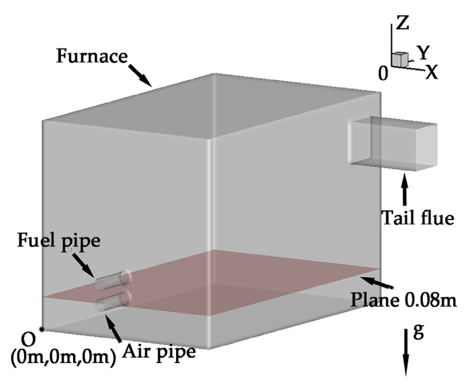
In the test model, gas fuel (propane) and air entered a burner through different pipes, and a mixture of gas fuel and air burned in the furnace. The furnace dimensions were 0.8 m in length, 0.5 m in width, and 0.5 m in height. The radius of the air pipe and fuel pipe was 0. 016 m. The coordinates of the air pipe center and fuel pipe center were 0.25, 0, and 0.1 m and 0.25, 0, and 0.15 m, respectively. The tail flue transverse dimensions were 0.15 m in width, 0.15 m in height, and 0.2 m in length. Figure 1 shows the geometry of the simulation model.
The simulation data from the plane at 0.08 m of the furnace height were used to test the proposed method and to present the reconstruction results.
Tetrahedral grids were employed for the fuel pipe and the air pipe. The furnace was structured by hexahedral grids to improve mesh quality. Five different mesh grids with node numbers of 452,997, 609,363, 784,370, 1,019,816 and 1,210,028, were used to test the mesh independency. The grid convergence index (GCI) [38] was also used in this test:
where is the safety factor and is the order of grid convergence. is the highest temperature in the simulation result using the k-grid, is the highest temperature in the simulation result using the k + 1 grid, is the grid nodes number in the k grid, and is the grid nodes number in the k + 1 grid.
The convergence condition is defined as follows:
GCI converges when .
The result is shown in Table 1.
As shown in Table 1, c in the 784,370 grid nodes is 0.91, and the 784,370, 1,019,816 and 1,210,028 grid nodes are in the asymptotic range of convergence. In consideration of the efficiency and accuracy, 784,370 grid nodes were used in the simulation model.
The basic governing equations in the simulation process were the conservation equations of mass, momentum, energy, species, and ideal gas state equation [39], which are as follows:
(1) Mass conservation equation:
(2) Momentum conservation equation:
(3) Energy conservation equation:
(4) Species conservation equation:
(5) Ideal gas state equation:
where is the density gas mixture, is time, is the velocity of the gas mixture, is the static pressure, is the stress tensor, is the gravitational body force, is the external body forces, is the energy content per unit mass of the gas mixture, is the effective conductivity, is the temperature of the gas mixture, is the enthalpy of the species i gas, is the diffusion flux of the species i gas, is the heat of other sources, is the mass fraction of the species i gas, is the net rate of production of the species i gas in chemical reactions, is the rate of creation with the addition of the dispersed phase plus any other sources, is the universal gas constant, and is the molecular weight of the species i gas.
In the simulations, the standard turbulence model and the second-order upwind difference scheme were used. The other model constants were set to the default values. The species model was set to “Species Transport”, and the mixture material was set to “propane–air”. The radiation model was set to “P1” and the absorption coefficient was set to “wsggm-domain-based”. The “Eddy-Dissipation” model was used as the turbulence–chemistry interaction model.
The solution method was “SIMPLE”. The gradient was set to “Least Squares Cell-Based”, the pressure was set to “Second Order”, and the momentum and turbulent kinetic energy were set to “Second-Order Upwind”. The “energy” residual convergence was set to 10-5, and the others were set to 10-3. Observation points temperature and mass balance were also important factors in the determination of convergence.
For boundary conditions, the outlet was set to “outflow”. The fuel inlet boundary was set to “velocity-inlet”, and the air inlet boundary was set to “velocity-inlet”. The boundary conditions of the walls were set as “Stationary Wall” and “No Slip”. The near-wall treatment was set as “Standard Wall Functions”. Considering the water-cooling jacket that is used in real applications, for convenience, the wall temperature was set as 343.15 K.
As the dataset shows features of the temperature field, it means a lot to the proposed method and directly influences the accuracy of the reconstruction results. Therefore, a wide range of boundary conditions were used to carry out a sufficient number of simulation results. A sample dataset was established by the CFD results whose boundary conditions were fuel velocities of 0.44, 0.54, …, 1.14 m/s, with the air velocities being determined by the excess air coefficient ().
Six test cases were also set up to test the reconstruction results. The boundary conditions of the test cases are shown in Table 2.
In order to test the proposed method in different conditions, firstly, a small fuel velocity 0.58m/s was used in this study. This was in the scope of 0.44 to 1.14 m/s, which was used for setting up the dataset. After that, 1.23 m/s was used to show the performance of the proposed method in the high-speed situation; 1.23 m/s was out of the range of 0.44 to 1.14 m/s, the reconstruction results in this boundary condition test whether the application range of the proposed method would be limited by the dataset boundary conditions. Furthermore, the CFD result with the fuel velocity set to 1.33 m/s and excess air coefficient set to 1.1 was used as a special test case.
3.2. Reconstruction Result
After setting up the sample dataset with the CFD simulation results, the POD basis vectors were extracted from it. Test cases were used to show the reconstruction result.
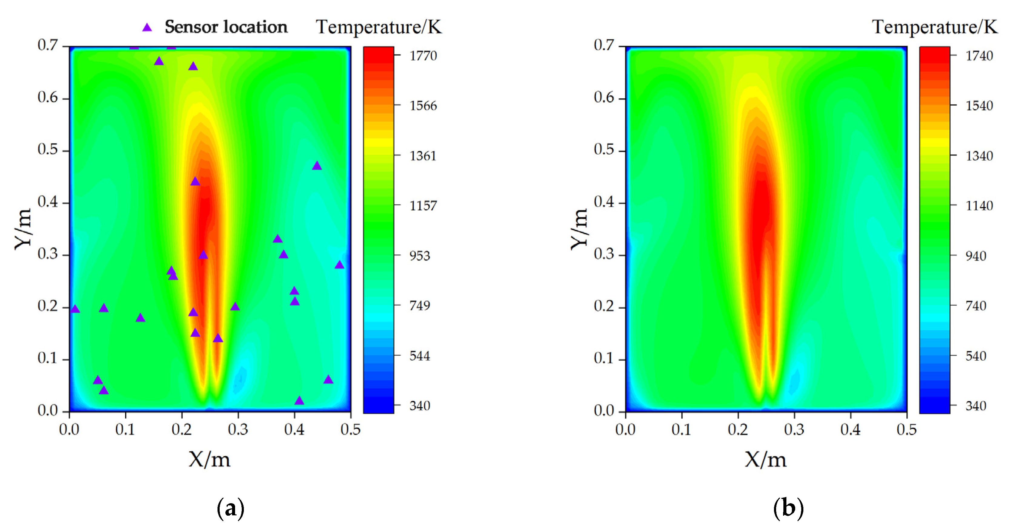
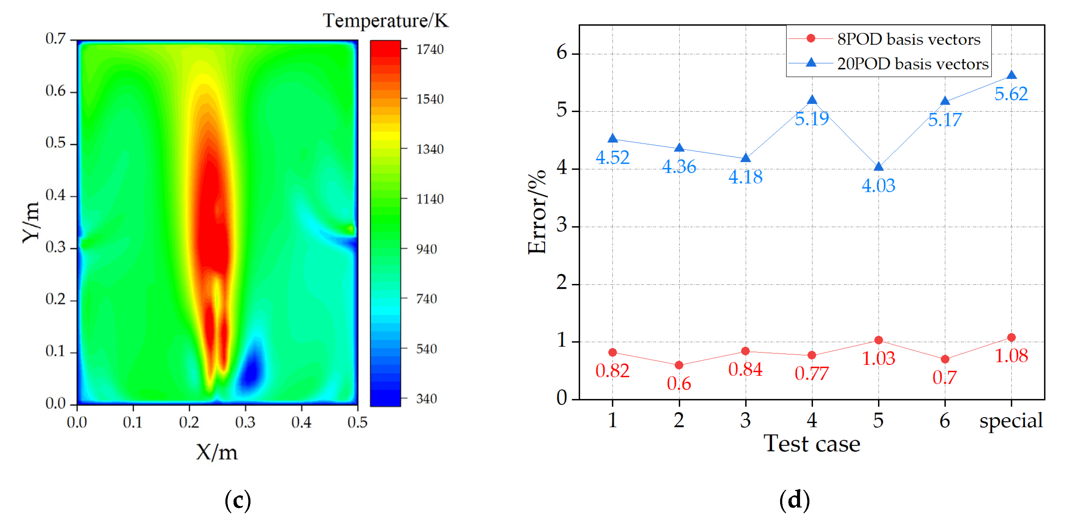
For reconstruction, 25 pieces of data were randomly extracted from the CFD results, and Gaussian noise was added to these data and the signal-to-noise ratio (SNR) was 40 dB. The results were used as the measurement data. In this special test case, the measurement data remained constant. Figure 2 shows the temperature contours with the simulation results and reconstruction results in the plane at 0.08 m.
As Figure 2 shows, the contours in Figure 2b are similar to those in Figure 2a, and the contours in Figure 2c are quite different from those in Figure 2a. When comes to Figure 2d, it is obvious that using eight POD basis vectors could result in a much better solution than using 20 POD basis vectors. Above all, Figure 2 indicates that the proposed method could be used in temperature field reconstruction, it also reveals that there are some important factors that can affect the reconstruction result and further study is needed.
Moreover, the boundary condition of the special test case is different from those used to set up the sample dataset. This result shows that the proposed method has a wide range of applications and a certain robustness.
3.3. Reconstruction Error Analysis
Equation (9) shows that the accuracy of the proposed method is associated with the number of POD basis vectors, sensor placement, and measurement noise. In the simulation test, measurement data were extracted from the CFD result. The measurement noise was artificially simulated by adding Gaussian noise to the sensor signal. These effects are discussed in this section.
3.3.1. Effect of the Number of POD Basis Vectors
In the reconstruction problem, the first few POD basis vectors contain most of the “energy”, and these basis vectors have a positive influence on the accuracy of the reconstruction result. The rest of the vectors contain less energy and are sensitive to noise. The noise may come from the measurement or calculation. In this situation, a large number of POD basis vectors means a high noise sensitivity. Therefore, in the reconstruction process, a proper number of POD basis vectors is needed.
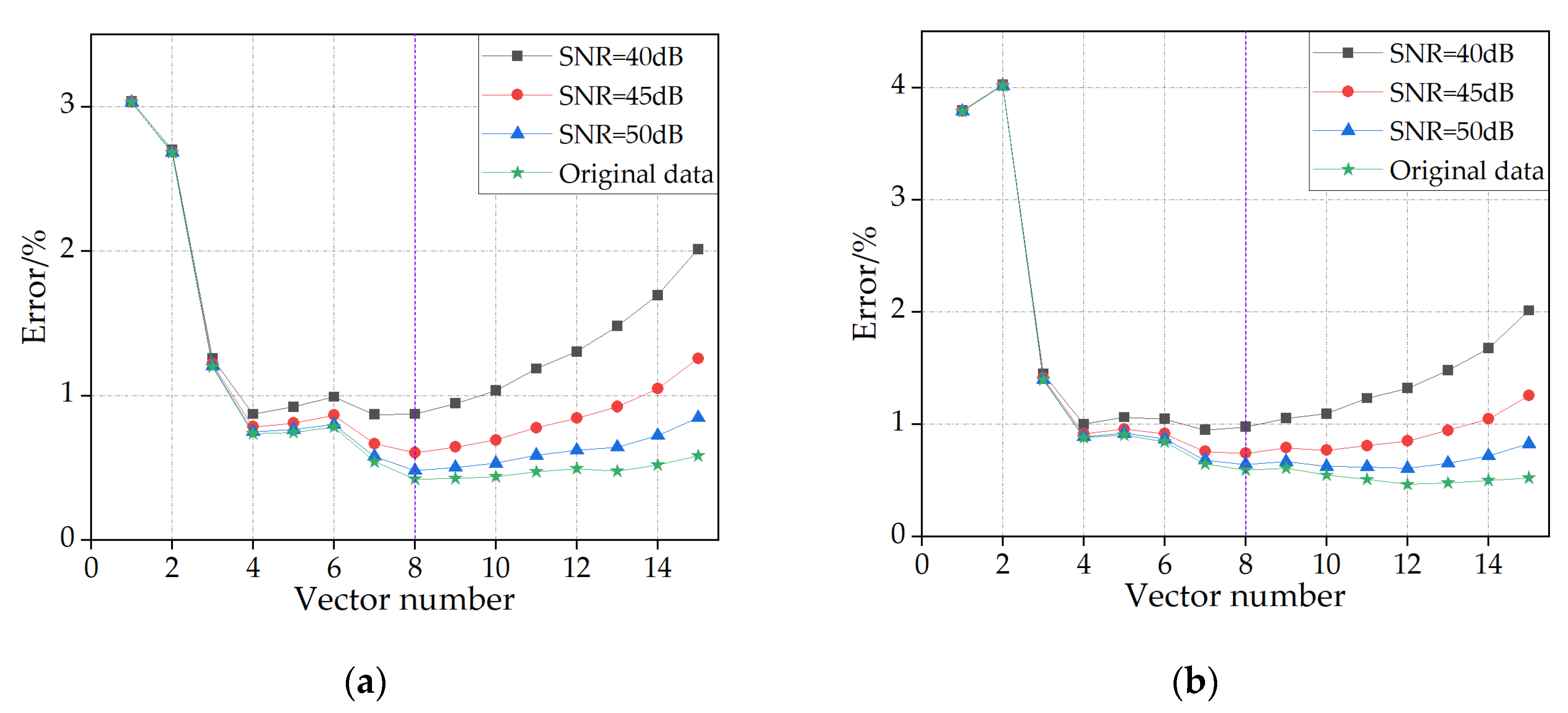
A test was set up to investigate the changes in the reconstruction error with different numbers of POD basis vectors. In this test, 25 sensors were placed in random locations, the number of POD basis vectors varied from 1 to 15, the SNR of the noise varied from 40 to 50 dB, and the original measurement data without noise were used for comparison. As the sensor location and the noise were randomized for different conditions, the averages of reconstruction results of 1000 runs were used to draw a general conclusion. Figure 3 shows the results for two test cases.
As shown in Figure 3, the reconstruction error decreased at first and then increased with a large number of vectors. This phenomenon is more pronounced when the noise level increases. In both test cases, a reconstruction error with eight POD basis vectors was acceptable.
Reconstruction errors with eight POD basis vectors and 25 sensors in different test cases are shown in Table 3.
As shown in Table 3, in all of the conditions, using the first eight basis vectors could obtain a balance between noise sensitivity and reconstruction accuracy. Therefore, in this simulation scenario, the first eight POD basis vectors resulted in better performance.
3.3.2. Effect of Sample Rate
The proposed method provides a new way of using limited measurement data to get temperature information. These measurement data play a very important role in the reconstruction process, so the number of sensors has an effect on the reconstruction accuracy to a certain extent.
In this simulation test, the number of nodes on the object plane was approximately 4000. All of these nodes can be seen as a measuring point. Considering the measurement cost and reconstruction accuracy, a certain number of sensors is needed.
As mentioned above, methods based on POD require sensor numbers equal to or larger than the total number of basis vectors used. With eight POD basis vectors used for reconstruction, a 0.1% sample rate (four sensors) and a 0.2% sample rate (eight sensors) were not suitable for this problem.
For a general conclusion, the averages of the reconstruction errors from 1000 runs under different noise levels were compared, as the sample rate increased from 0.3% to 1.2%. These results are presented in Figure 4.
As shown in Figure 4, in all conditions, it is obvious that the reconstruction error decreased as the sample number increased from 0.3% to 1.2%. The greater the number of sensors used, the better the reconstruction solution. Another remarkable outcome is that using a high sample rate resulted in a decrease in the effect of noise. This indicates that, even with measurement noise, using the proposed method and moderate measurement data can yield a good reconstruction solution.
Reconstruction errors with a 0.3% sample rate (12 sensors) for different test cases are shown in Table 4.
As shown in Table 4, when the sample rate was 0.3% (12 sensors), the reconstruction errors were all less than 3%, which is an acceptable result. Considering the reconstruction accuracy and measurement cost, in this simulation test, a sample rate of 0.3% (12 sensors) was used in following analysis.
3.3.3. Effect of Sensor Placement
Sensor placement has a profound influence on reconstruction accuracy. Given random locations, different sensor distributions can result in different reconstruction solutions, and the errors between them are often larger than 1%. Optimal sensor placement can yield a better reconstruction result and lower measurement cost.
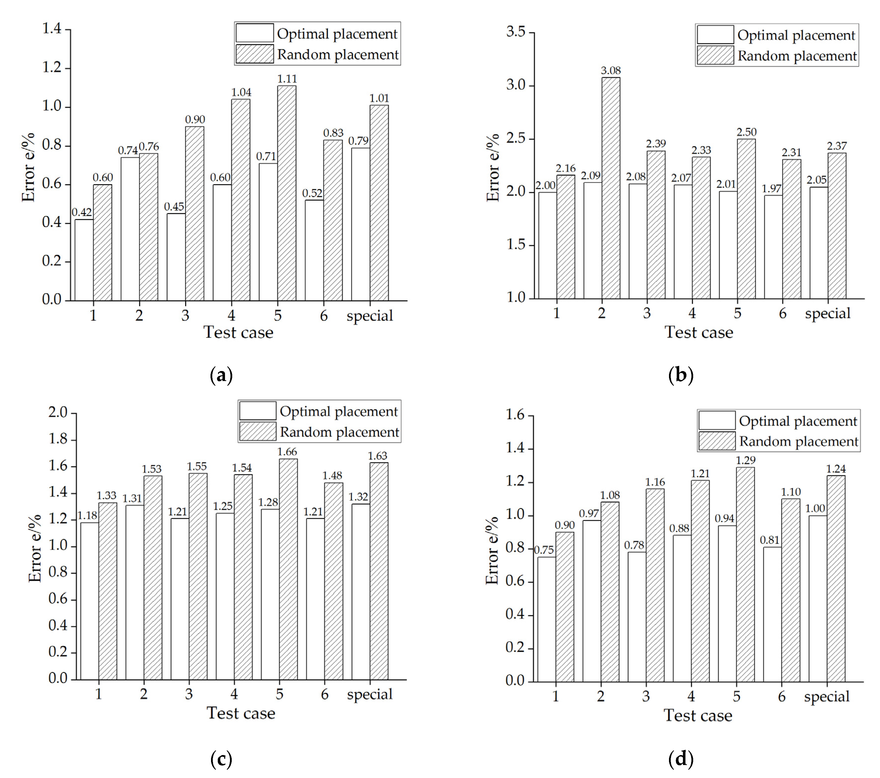
The proposed sensor placement optimization algorithm was tested by calculating the reconstruction results for optimal sensor placement and comparing them with those for random placement. The first eight basis vectors and 12 sensors were used in the reconstruction. Noise was also added to the original measurement data. The averages of the reconstruction errors from 1000 runs were used to obtain the overall result. Figure 5 compares the results for different test cases.
As can be observed from the figure above, in all six test cases, optimal sensor placement could yield a better reconstruction resolution than placing sensors randomly. Although optimal sensor placement may not obtain the best solution, this approach is more adaptable in different conditions and is less sensitive to noise.
Overall, the results in this section suggest that the proposed method is feasible and can yield an acceptable reconstruction solution. The next section, therefore, shows the performance of the proposed method in a gas combustion experiment.
4. Experimental Test
Combustion experiments were set up to validate the performance of the proposed method. Parts of the experimental facilities and combustion flame are shown in Figure 6.
4.1. Experimental System
The experimental system had two main parts: a combustion system and measurement system.
4.1.1. Combustion System
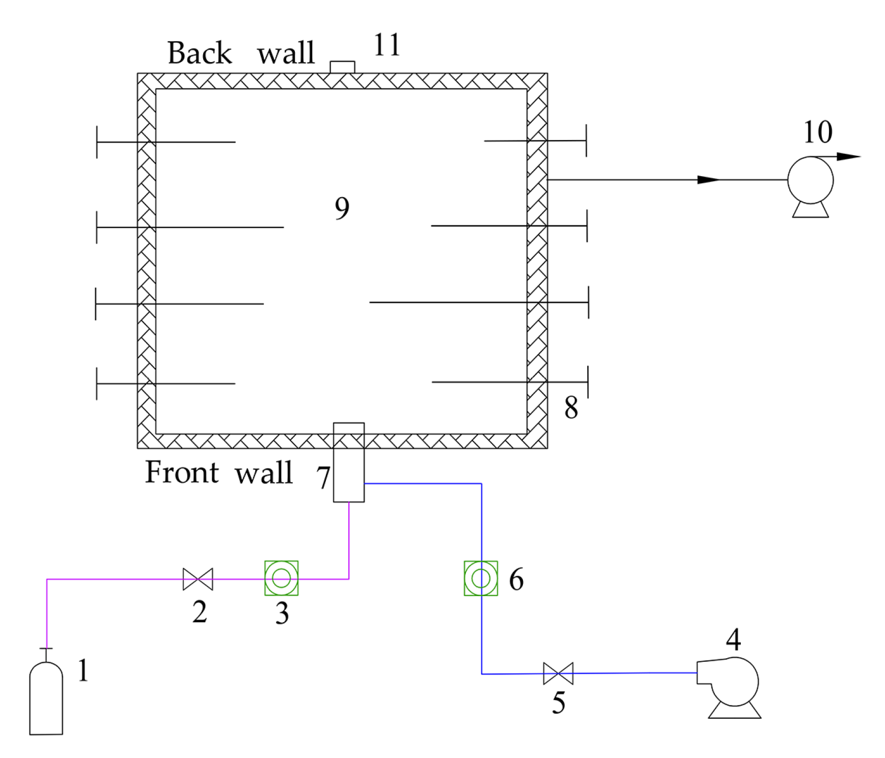
The combustion system was composed of the combustion chamber, air pipeline, fuel pipeline, and tail flue. Figure 7 shows the layout of the combustion system.
As shown in Figure 7, gas fuel (propane) was supplied by a compressed gas cylinder, and combustion air was provided by a CX-75 5.5 medium-pressure fan. Combustion conditions were changed by setting different air–fuel ratios.
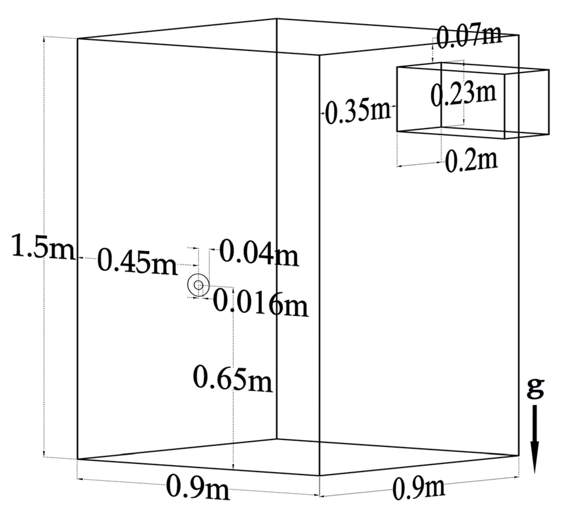
Propane and air entered the burner through different pipes, and the mixture of gas fuel and air was ignited at the outlet of the burner and then burned in the combustion chamber. The chamber dimensions were 0.9 m in length, 0.9 m in width, and 1.5 m in height. The radius of the burner was 0.04 m, and the radius of the fuel line was 0.016 m. In order to observe the flame, there was an observation hole on the back wall; its location was directly across the gas burner. Hot smoke was exhausted by an induced draft fan through the tail flue. The tail flue transverse dimensions were 0.2 m in width and 0.23 m in height. Several spray type attemperators in the tail flue were used to lower the temperature of hot smoke. Data from the plane at 0.65 m height was used to validate the reconstruction results.
Figure 8 shows the geometry of the combustion chamber.
4.1.2. Measurement System
The temperature was measured by three different types of thermocouples, whose parameters are reported in Table 5.
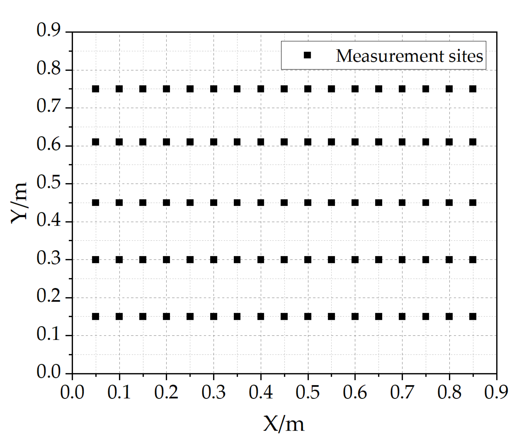
The measurement site can be changed by adjusting the insertion depth of the thermocouples. There were 85 possible measurement sites on the plane at 0.65 m height. The Y coordinates of these sites were 0.15, 0.30, 0.45, 0.61, and 0.75 m, respectively, and the adjacent X coordinates differed by 0.05 m. The measurement sites are shown in Figure 9.
The DAM-3038 data acquisition module was used to collect temperature measurement data. This kind of module has eight input channels. The sample rate is 10 sps, and the resolution is 16 bits. The millivolt voltage electric signal was converted to a digital signal and transferred to a laptop PC.
4.2. Experimental Procedure
Measurement data from the combustion experiment were used to test the proposed method. The experimental procedure is summarized below.
- A simulation model with the same physical dimensions as those of the combustion system was set up to obtain POD basis vectors. Boundary conditions and the calculated model, which were close to the actual constraints, were set up. Calculation model parameter settings were the same as described in Section 3. In the mesh independency test, a mesh with 2,641,471 grid nodes was in the asymptotic range of convergence, and 10 measurement data on the plane at 0.65 m height were used to compare with the simulation result. The relative error between the simulation result and measurements was 1.3%. As a result, 2,641,471 grid nodes were used in this experiment test. Fuel velocities were set to 0.44, 0.54, 0.64, and 0.74 m/s. The excess air coefficient was set to 0.8, 0.9, 1, 1.1, and 1.2. A 20 × 85 sample dataset was established with the simulation results, and POD basis vectors were extracted from it. In this experiment, when the basis vector number and sensor number increased to six, reconstruction errors tended to be stable. Finally, optimal sensor placement was calculated by the proposed optimization algorithm.
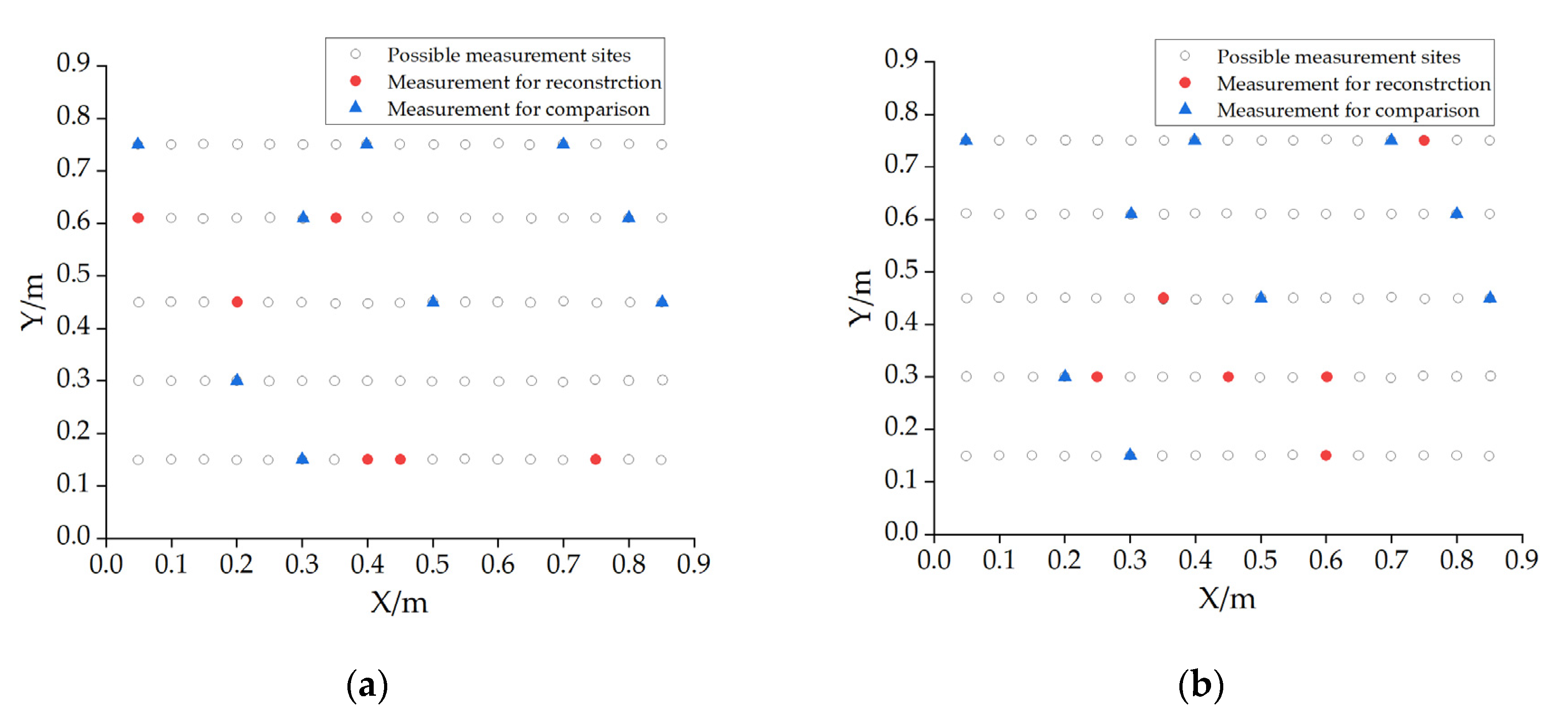
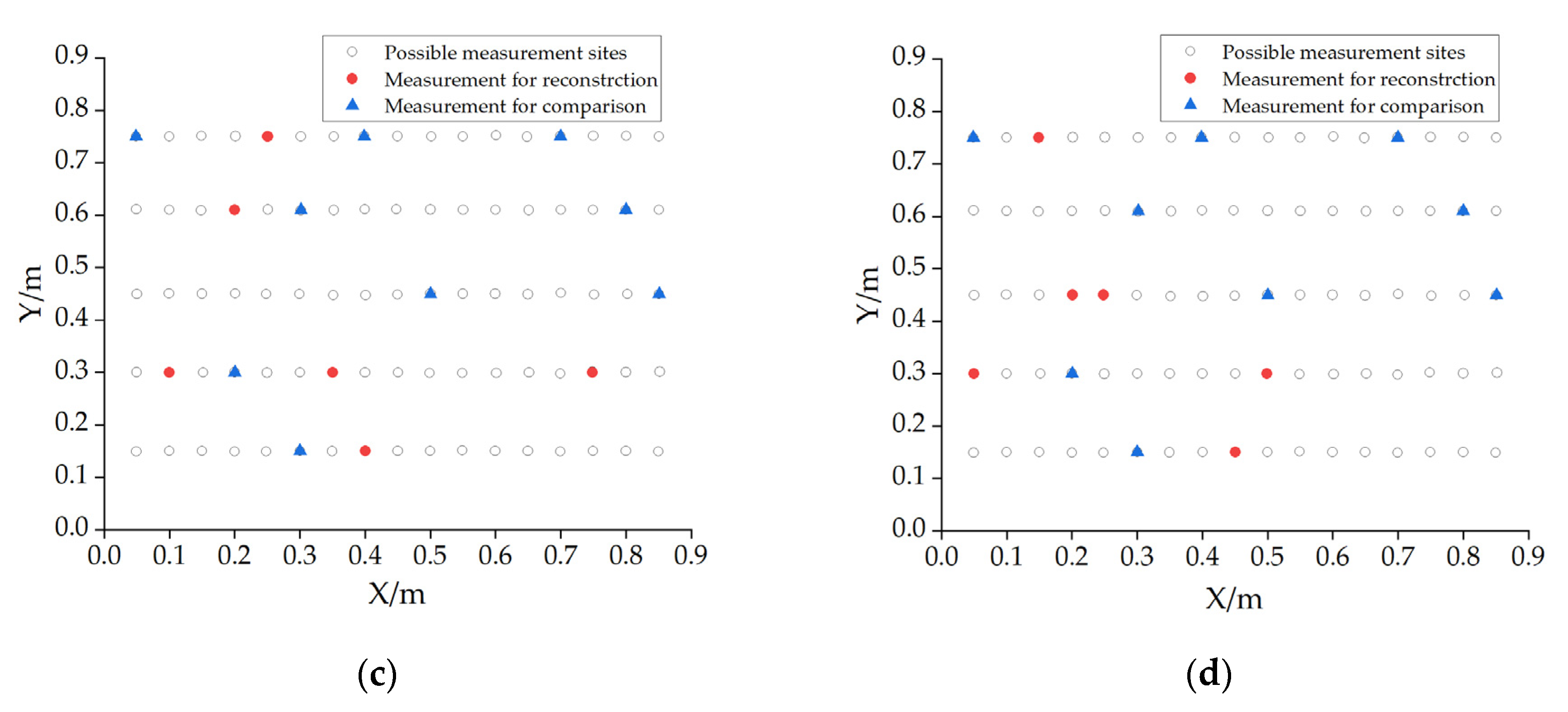
- As shown in Figure 9, 10 thermocouples can measure the temperature at the same time. The sensor placement optimization algorithm was tested by comparing the reconstruction results from optimal placement with those from three random placements. A combustion experiment was set up with a fuel mass flow of 1.5 m/s and an excess air coefficient of 1.25, and when combustion was stable, six temperature values were measured to reconstruct the temperature field. Another nine temperature values were used to compare with the reconstruction data. These temperature values were collected by two measurements. Sensor locations in different cases are shown in Figure 10.Furthermore, all temperature values in the possible measurement sites were collected to validate the overall reconstruction result. First, 10 temperature values in different locations were collected in a measurement; then, after changing sensor locations and ensuring that the measurement was stable, another 10 temperature values were collected. The measurements were repeated until all values were collected from 85 sites. Each measurement took 10 s, and the averages of the measurement data were used to test the proposed method.
- The measurement data and POD basis vectors were used to reconstruction the temperature field with the proposed method.
4.3. Experimental Results
First, measurement data for the optimal placement are compared with data for three random placements in Table 5.
Temperature deviations in the different measurements are quite small, and the temperature field can be deemed to be stable. The averages of four measurements were used for comparison with reconstruction results.
Then, the temperature field can be calculated by using measurement data for reconstruction in different placements and the proposed method. Table 6 shows the reconstruction errors.
As shown in Table 7, it is remarkable that optimal placement yielded a much better reconstruction result than the random placements.
Finally, all values of the 85 possible measurement locations were used to test the proposed method. Reconstruction errors for optimal placement and three random placements are compared in Table 8.
Table 8 shows that the proposed method can yield a reliable reconstruction solution in experimental condition. These results further support the effectiveness of the sensor placement optimization algorithm.
5. Conclusions
Reliable temperature information is necessary for many industrial processes. A temperature field reconstruction method based on proper orthogonal decomposition is proposed in this study. Both the simulation results and experimental results show that the proposed method is feasible and reliable. The main findings of this study can be summarized as follows:
- In simulation tests and experimental tests, the proposed method can rapidly reconstruct the temperature field with limited measurement data. It can dramatically reduce computation complexity and measurement cost. It also has good adaptability and can apply to real-time applications.
- The dataset which is used to generate the POD basis vector plays a very important role in the proposed method. All the methods used in this study are based on it. When using CFD results to set up the dataset, sampling a wide range of boundary conditions which can cover most of working conditions in the flow field is of vital importance.
- POD basis vectors can be extracted from a high-dimensional experience dataset. The first few basis vectors carry most of the useful information. With the use of a large number of basis vectors, too much useless information is introduced to the reconstruction process, and the reconstruction result is much more sensitive to the noise. Thus, it is necessary to obtain a balance between reconstruction accuracy and noise sensitivity. “Energy”, which was mentioned in Section 3.3.1, can be used in finding the balance point. In the experience of this study, the vectors which contain “energy” lower than 0.1% are more sensitive to noise, so avoiding using these vectors will be better.
- The proposed method needs little measurement data to yield an acceptable reconstruction result. The sensor number has some effect on the reconstruction result: the greater the number of sensors used, the better result. However, this effect decreases when the number of sensors increases to a certain threshold. Therefore, the balance between measurement cost and reconstruction accuracy requires the appropriate numbers of sensors.
- When only a few sensors are used for reconstruction, sensor placement has a great influence on reconstruction accuracy. The sensor placement optimization algorithm was also tested in this study. The results show that optimal placement can yield a much more accurate result than random placement. The optimal sensor placement algorithm in this paper may not obtain the best solution, but it is more adaptable in different conditions and less sensitive to noise.
- Noise has a great effect on the reconstruction error. However, the proposed method can also yield an acceptable reconstruction result in the presence of noise, and this effect tends to decrease when using a large number of sensors.
Furthermore, the present study lays the groundwork for future research into some interesting fields with several objectives, including the following:
- The feasibility of using the proposed method to reconstruct a temperature field was tested in this study. In order to show more features of the object field, a wide span of boundary conditions was used to set up the dataset. This is helpful for generating POD basis vectors, but how to constitute a dataset more efficiently remains to be addressed. Further research could focus on the source of experience data, efficient dataset sampling, and the influence of noise in the dataset.
- Testing the feasibility of finding a sensor placement optimization algorithm that can yield a much better reconstruction result.
- Combining the proposed method and modern measurement techniques.
- Using the experience gained from this study to develop a new method to reconstruct the temperature field in three-dimensional space.
Author Contributions
Conceptualization, M.C. and S.L.; Data curation, M.C.; Formal analysis, M.C.; Funding acquisition, S.L.; Methodology, M.C.; Project administration, S.L.; Software, M.C.; Supervision, S.L.; Validation, M.C., S.S., Y.Z. and Z.L.; Writing—original draft, M.C. All authors have read and agreed to the published version of the manuscript.
Funding
This study was funded by the National Natural Science Foundation of China (Grant No. 61871181) and supported by the Fundamental Research Funds for the Central Universities (2019QN013).
Conflicts of Interest
The authors declare no conflict of interest.
References
- Jia, R.; Xiong, Q.; Xu, G.; Wang, K.; Liang, S. A method for two-dimensional temperature field distribution reconstruction. Appl. Therm. Eng. 2017, 111, 961–967. [Google Scholar] [CrossRef]
- Bramanti, M.; Salerno, E.A.; Tonazzini, A.; Pasini, S.; Gray, A. An acoustic pyrometer system for tomographic thermal imaging in power plant boilers. IEEE Trans. Instrum. Meas. 1996, 45, 159–167. [Google Scholar] [CrossRef]
- Huang, Y.S.; Huang, Y.P.; Huang, K.N.; Young, M.S. An accurate air temperature measurement system based on an envelope pulsed ultrasonic time-of-flight technique. Rev. Sci. Instrum. 2007, 78, 115102. [Google Scholar] [CrossRef] [PubMed]
- Lou, C.; Zhou, H.C. Deduction of the two-dimensional distribution of temperature in a cross section of a boiler furnace from images of flame radiation. Combust. Flame 2005, 143, 97–105. [Google Scholar] [CrossRef]
- Guariglia, E. Primality, Fractality and Image Analysis. Entropy 2019, 21, 304. [Google Scholar] [CrossRef] [Green Version]
- Guido, R.C. A note on a practical relationship between filters coefficients and the scaling and wavelet functions of the discrete wavelet transform. Appl. Math. Lett. 2011, 24, 1257–1259. [Google Scholar] [CrossRef]
- Hentschel, H.; Procaccia, I. The infinite number of generalized dimensions of fractals and strange attractors. Phys. D Nonlinear Phenom. 1983, 8, 435–444. [Google Scholar] [CrossRef]
- Mallat, S. A theory for multiresolution signal decomposition: The wavelet representation. IEEE Trans. Pattern Anal. Mach. Intell. 1989, 11, 674693. [Google Scholar] [CrossRef] [Green Version]
- Guariglia, E.; Silvestrov, S. Fractional-Wavelet Analysis of Positive definite Distributions and Wavelets on D’(C). In Engineering Mathematics II; Silvestrov, R., Ed.; Springer: Berlin, Germany, 2016; pp. 337–353. [Google Scholar]
- Guariglia, E. Entropy and Fractal Antennas. Entropy 2016, 18, 84. [Google Scholar] [CrossRef]
- Guariglia, E. Harmonic Sierpinski Gasket and Applications. Entropy 2018, 20, 714. [Google Scholar] [CrossRef] [Green Version]
- Kirby, M. Geometric Data Analysis: An Empirical Approach to Dimensionality Reduction and the Study of Patterns; John Wlley: New York, NY, USA, 2001; pp. 1–144. [Google Scholar]
- Pearson, K. On lines and planes of closest fit to systems of points in space. Philos. Mag. 1901, 2, 559–572. [Google Scholar] [CrossRef] [Green Version]
- Aharon, M.; Elad, M.; Bruckstein, A. K-SVD: An Algorithm for Designing Overcomplete Dictionaries for Sparse Representation. IEEE Trans. Signal Process. 2006, 54, 4311–4322. [Google Scholar] [CrossRef]
- Berkooz, G.; Holmes, P.; Lumley, J.L. The Proper Orthogonal Decomposition in the Analysis of Turbulent Flows. Annu. Rev. Fluid Mech. 1993, 25, 539–575. [Google Scholar] [CrossRef]
- Luh, G.C.; Lin, C.Y. PCA based immune networks for human face recognition. Appl. Soft Comput. 2011, 11, 1743–1752. [Google Scholar] [CrossRef]
- Zhang, S.C.; Ji, R.R.; Cai, L.; Gao, X.B. Face sketch aging via aging oriented principal component analysis. Pattern Recognit. Lett. 2018, 109, 65–71. [Google Scholar] [CrossRef]
- Polansky, J.; Wang, M. Proper Orthogonal Decomposition as a technique for identifying two-phase flow pattern based on electrical impedance tomography. Flow Meas. Instrum. 2017, 53, 126–132. [Google Scholar] [CrossRef] [Green Version]
- Xu, C.O.; Ou, Y.S.; Schuster, E. Sequential linear quadratic control of bilinear parabolic PDEs based on POD model reduction. Automatica 2011, 47, 418–426. [Google Scholar] [CrossRef]
- Sun, X.H.; Xu, M.H. Optimal control of water flooding reservoir using proper orthogonal decomposition. J. Comput. Appl. Math. 2017, 320, 120–137. [Google Scholar] [CrossRef]
- Lumley, J. The structure of inhomogeneous turbulence. Atmos. Turbul. Radio Wave Propag. 1967, 2, 166–178. [Google Scholar]
- Sirovich, L. Turbulence and the dynamics of coherent structures. I. Coherent structures. Q. Appl. Math. 1987, 45, 561–571. [Google Scholar] [CrossRef] [Green Version]
- Willcox, K. Unsteady flow sensing and estimation via the gappy proper orthogonal decomposition. Comput. Fluids 2006, 35, 208–226. [Google Scholar] [CrossRef] [Green Version]
- Allery, C.; Beghein, C.; Hamdouni, A. On investigation of particle dispersion by a POD approach. Int. Appl. Mech. 2008, 44, 110–119. [Google Scholar] [CrossRef]
- Qin, L.; Liu, S.; Long, T.; Shahzad, M.A.; Schlaberg, H.I.; Yan, S.A. Wind field reconstruction using dimension-reduction of CFD data with experimental validation. Energy 2018, 151, 272–288. [Google Scholar] [CrossRef]
- Sun, S.; Liu, S.; Zhang, G. The Rapid Establishment of Large Wind Fields via an Inverse Process. Appl. Sci. 2019, 9, 2847. [Google Scholar] [CrossRef] [Green Version]
- Yildirim, B.; Chryssostomidis, C.; Karniadakis, G.E. Efficient sensor placement for ocean measurements using low-dimensional concepts. Ocean Model. 2009, 27, 160–173. [Google Scholar] [CrossRef] [Green Version]
- Raveh, D.E. Reduced-Order Models for Nonlinear Unsteady Aerodynamics. AIAA J. 2012, 39, 1417–1429. [Google Scholar] [CrossRef]
- Mifsud, M.J.; MacManus, D.G.; Shaw, S.T. A variable-fidelity aerodynamic model using proper orthogonal decomposition. Int. J. Numer. Methods Fluids 2016, 82, 646–663. [Google Scholar] [CrossRef] [Green Version]
- Zhang, Y.W.; Bellingham, J.G. An efficient method of selecting ocean observing locations for capturing the leading modes and reconstructing the full field. J. Geophys. Res.Oceans 2008, 113, C04005. [Google Scholar] [CrossRef] [Green Version]
- Zhang, Z.Q.; Yang, X.; Lin, G. POD-Based Constrained Sensor Placement and Field Reconstruction from Noisy Wind Measurements: A Perturbation Study. Mathematics 2016, 4, 26. [Google Scholar] [CrossRef] [Green Version]
- Lu, K.; Jin, Y.L.; Chen, Y.S.; Yang, Y.F.; Hou, L.; Zhang, Z.Y.; Li, Z.G.; Fu, C. Review for order reduction based on proper orthogonal decomposition and outlooks of applications in mechanical systems. Mech. Syst. Signal Pr. 2019, 123, 264–297. [Google Scholar] [CrossRef]
- Zhang, X. Matrix Analysis and Application; Tsinghua University Press: Bejing, China, 2009; pp. 453–471. (In Chinese) [Google Scholar]
- Everson, R.; Sirovich, L. Karhunen-Loeve procedure for gappy data. J. Opt. Soc. Am. A Opt. Image Sci. Vis. 1995, 12, 1657–1664. [Google Scholar] [CrossRef] [Green Version]
- David, C.; Lay, S.R.L.; Judi, J.M. LINEAR ALGEBRA AND ITS APPLICATIONS; PEARSON: New York, NY, USA, 2015; pp. 1–162. [Google Scholar]
- Semaan, R. Optimal sensor placement using machine learning. Comput. Fluids 2017, 159, 167–176. [Google Scholar] [CrossRef] [Green Version]
- Tropp, J.A. Greed is good: Algorithmic results for sparse approximation. IEEE Trans. Inf. Theory 2004, 50, 2231–2242. [Google Scholar] [CrossRef] [Green Version]
- Roache, P.J. Quatification of uncertainty in computational fluid dynamics. Annu. Rev. Fluid Mech. 1997, 29, 123–160. [Google Scholar] [CrossRef] [Green Version]
- Anderson, J.D. COMPUTATIONAL FLUID DYNAMICS: The Basics with Applications; McGraw-Hill: New York, NY, USA, 1995; pp. 37–93. [Google Scholar]
Figure 1.
Schematic diagram of the simulation model.

Figure 2.
Comparisons of the reconstruction results. (a) Simulation results in the special test case, (b) reconstruction results in the special test case (eight proper orthogonal decomposition (POD) basis vectors), (c) reconstruction result in special test case (20 POD basis vectors), and (d) reconstruction errors in different test cases.


Figure 3.
Comparison of reconstruction errors between different POD basis vectors with different noise levels (original measurement data, signal-to-noise ratio (SNR) = 40 dB, SNR = 45 dB, SNR = 50 dB). (a) Comparison in test case 2. (b) Comparison in test case 4.
Figure 3.
Comparison of reconstruction errors between different POD basis vectors with different noise levels (original measurement data, signal-to-noise ratio (SNR) = 40 dB, SNR = 45 dB, SNR = 50 dB). (a) Comparison in test case 2. (b) Comparison in test case 4.

Figure 4.
Comparison of reconstruction errors between different sample rates with different noise levels (original measurement data, SNR = 40 dB, SNR = 45 dB, SNR = 50 dB). (a) Comparison in test case 1. (b) Comparison in test case 6.
Figure 4.
Comparison of reconstruction errors between different sample rates with different noise levels (original measurement data, SNR = 40 dB, SNR = 45 dB, SNR = 50 dB). (a) Comparison in test case 1. (b) Comparison in test case 6.

Figure 5.
Comparison of reconstruction errors between the optimal placement and random placements in different test cases with different levels of noise. (a) Original measurement data; (b) SNR = 40 dB; (c) SNR = 45 dB; (d) SNR = 50 dB.
Figure 5.
Comparison of reconstruction errors between the optimal placement and random placements in different test cases with different levels of noise. (a) Original measurement data; (b) SNR = 40 dB; (c) SNR = 45 dB; (d) SNR = 50 dB.

Figure 6.
(a) Experiment facilities: (1) gas burner, (2) air line, (3) fuel line, (4) gas valve, (5) tail flue, (6) spray type attemperator (7) thermal couples; (b) resulting flame (observation hole is on the back wall, directly across the gas burner).
Figure 6.
(a) Experiment facilities: (1) gas burner, (2) air line, (3) fuel line, (4) gas valve, (5) tail flue, (6) spray type attemperator (7) thermal couples; (b) resulting flame (observation hole is on the back wall, directly across the gas burner).

Figure 7.
Layout of the combustion system. (1) Compressed gas cylinder, (2) gas valve, (3) gas flowmeter, (4) air fan, (5) air valve, (6) hotwire anemometer, (7) gas burner, (8) thermal couples, (9) combustion chamber, (10) induced draft fan, and (11) observation hole.
Figure 7.
Layout of the combustion system. (1) Compressed gas cylinder, (2) gas valve, (3) gas flowmeter, (4) air fan, (5) air valve, (6) hotwire anemometer, (7) gas burner, (8) thermal couples, (9) combustion chamber, (10) induced draft fan, and (11) observation hole.

Figure 8.
Geometry of the combustion chamber.

Figure 9.
Measurement sites.

Figure 10.
Sensor placements. (a) Optimal placement, (b) random placement 1, (c) random placement 2, and (d) random placement 3.
Figure 10.
Sensor placements. (a) Optimal placement, (b) random placement 1, (c) random placement 2, and (d) random placement 3.


Table 1.
GCI convergence test.
| Nodes Number | GCI (%) | c | |
|---|---|---|---|
| 452,297 | 2.59 | 1.21 | -- |
| 609,363 | 2 | 1.18 | 0.65 |
| 784,370 | 2.18 | 1.19 | 0.91 |
| 1,019,816 | 2.33 | 1.12 | 0.95 |
| 1,210,028 | -- | -- | -- |
Table 2.
Boundary conditions of six test cases.
| Test Case Number | Fuel Velocities (m/s) | Excess Air Coefficient |
|---|---|---|
| 1 | 0.58 | 0.75 |
| 2 | 0.58 | 1.25 |
| 3 | 0.58 | 1.40 |
| 4 | 1.23 | 0.75 |
| 5 | 1.23 | 1.25 |
| 6 | 1.23 | 1.40 |
Table 3.
Reconstruction errors (%) in seven test cases with eight POD basis vectors.
| Test Case Number | Original Data | SNR = 40 dB | SNR = 45 dB | SNR = 50 dB |
|---|---|---|---|---|
| 1 | 0.35 | 0.84 | 0.56 | 0.43 |
| 2 | 0.42 | 0.87 | 0.60 | 0.48 |
| 3 | 0.53 | 0.94 | 0.68 | 0.68 |
| 4 | 0.59 | 0.97 | 0.74 | 0.64 |
| 5 | 0.66 | 1.01 | 0.79 | 0.71 |
| 6 | 0.51 | 0.92 | 0.67 | 0.57 |
| special test case | 0.60 | 0.98 | 0.73 | 0.64 |
Table 4.
Reconstruction errors (%) in seven test cases with a 0.3% sample rate (12 sensors).
| Test Case Number | Original Data | SNR = 40 dB | SNR = 45dB | SNR = 50 dB |
|---|---|---|---|---|
| 1 | 0.59 | 2.11 | 1.38 | 0.90 |
| 2 | 0.70 | 2.18 | 1.40 | 1.00 |
| 3 | 0.84 | 2.20 | 1.43 | 1.09 |
| 4 | 1.05 | 2.35 | 1.58 | 1.26 |
| 5 | 1.15 | 2.42 | 1.67 | 1.35 |
| 6 | 0.84 | 2.31 | 1.46 | 1.09 |
| special test case | 0.98 | 2.53 | 1.59 | 1.23 |
Table 5.
Parameters of thermocouples.
| Type | Index Number | Outside Diameter (mm) | Length (mm) | Range (K) | Number |
|---|---|---|---|---|---|
| HT-116 | K | 12 | 700 | 273.15–1523.15 | 7 |
| HT-129 | S | 12 | 700 | 273.15–1773.15 | 1 |
| WRR-130 | B | 12 | 1000 | 273.15–2073.15 | 2 |
Table 6.
Temperature values (K) for test reconstruction result.
| Position | Optimal | Random 1 | Random 2 | Random 3 |
|---|---|---|---|---|
| 1 | 955.46 | 958.24 | 957.88 | 956.29 |
| 2 | 1028.13 | 1026.36 | 1025.46 | 1027.54 |
| 3 | 1012.98 | 1013.56 | 1017.76 | 1015.22 |
| 4 | 1420.86 | 1424.92 | 1425.73 | 1424.18 |
| 5 | 1119.37 | 1118.58 | 1126.75 | 1124.71 |
| 6 | 1191.33 | 1186.57 | 1186.58 | 1185.99 |
| 7 | 1112.33 | 1111.47 | 1107.12 | 1109.26 |
| 8 | 1332.85 | 1330.16 | 1330.65 | 1332.44 |
| 9 | 1174.38 | 1173.99 | 1177.79 | 1175.83 |
Table 7.
Reconstruction errors (%) for 9 positions.
| Sensor Placement | Error |
|---|---|
| Optimal placement | 1.77 |
| Random placement 1 | 2.23 |
| Random placement 2 | 7.76 |
| Random placement 3 | 22.62 |
Table 8.
Reconstruction errors (%) for 85 positions.
| Sensor Placement | Error |
|---|---|
| Optimal placement | 1.94 |
| Random placement 1 | 8.43 |
| Random placement 2 | 3.68 |
| Random placement 3 | 16.83 |
© 2020 by the authors. Licensee MDPI, Basel, Switzerland. This article is an open access article distributed under the terms and conditions of the Creative Commons Attribution (CC BY) license (http://creativecommons.org/licenses/by/4.0/).
Share and Cite
MDPI and ACS Style
Chen, M.; Liu, S.; Sun, S.; Liu, Z.; Zhao, Y. Rapid Reconstruction of Simulated and Experimental Temperature Fields Based on Proper Orthogonal Decomposition. Appl. Sci. 2020, 10, 3729. https://doi.org/10.3390/app10113729
AMA Style
Chen M, Liu S, Sun S, Liu Z, Zhao Y. Rapid Reconstruction of Simulated and Experimental Temperature Fields Based on Proper Orthogonal Decomposition. Applied Sciences. 2020; 10(11):3729. https://doi.org/10.3390/app10113729
Chicago/Turabian StyleChen, Minxin, Shi Liu, Shanxun Sun, Zhaoyu Liu, and Yu Zhao. 2020. "Rapid Reconstruction of Simulated and Experimental Temperature Fields Based on Proper Orthogonal Decomposition" Applied Sciences 10, no. 11: 3729. https://doi.org/10.3390/app10113729
Note that from the first issue of 2016, this journal uses article numbers instead of page numbers. See further details here.