Time Domain Room Acoustic Solver with Fourth-Order Explicit FEM Using Modified Time Integration


1
Technical Research Institute, Hazama Ando Corporation, Tsukuba 305-0822, Japan
2
Environmental Acoustics Laboratory, Department of Architecture, Graduate School of Engineering, Kobe University, Kobe 657-8501, Japan
*
Author to whom correspondence should be addressed.
Appl. Sci. 2020, 10(11), 3750; https://doi.org/10.3390/app10113750
Submission received: 16 April 2020
/
Revised: 24 May 2020
/
Accepted: 25 May 2020
/
Published: 28 May 2020
(This article belongs to the Special Issue Advances in Architectural Acoustics)
Abstract
:This paper presents a proposal of a time domain room acoustic solver using novel fourth-order accurate explicit time domain finite element method (TD-FEM), with demonstration of its applicability for practical room acoustic problems. Although time domain wave acoustic methods have been extremely attractive in recent years as room acoustic design tools, a computationally efficient solver is demanded to reduce their overly large computational costs for practical applications. Earlier, the authors proposed an efficient room acoustic solver using explicit TD-FEM having fourth-order accuracy in both space and time using low-order discretization techniques. Nevertheless, this conventional method only achieves fourth-order accuracy in time when using only square or cubic elements. That achievement markedly impairs the benefits of FEM with geometrical flexibility. As described herein, that difficulty is solved by construction of a specially designed time-integration method for time discretization. The proposed method can use irregularly shaped elements while maintaining fourth-order accuracy in time without additional computational complexity compared to the conventional method. The dispersion and dissipation characteristics of the proposed method are examined respectively both theoretically and numerically. Moreover, the practicality of the method for solving room acoustic problems at kilohertz frequencies is presented via two numerical examples of acoustic simulations in a rectangular sound field including complex sound diffusers and in a complexly shaped concert hall.
1. Introduction
1.1. Study Background
For room acoustic design, it is crucially important to predict accurate impulse responses to provide comfortable acoustic environments necessary for various rooms such as concert halls, offices, and classrooms. Using impulse responses, one can design room acoustics via visualization and auralization of sound fields as well as calculating room acoustic parameters such as reverberation times and the speech transmission index. Computer simulation methods are indispensable tools for room acoustic modeling because they can virtually simulate acoustics in architectural spaces. Furthermore, simulation can facilitate parametric studies more readily than scale model experiments for designing basic room shapes and interior finishes that is, selection of acoustical absorptive or reflective materials [1]. Geometrical acoustics simulation methods have flourished since their original proposition in the 1960s [2,3] to today, as a practical room acoustic design tool [4,5]. Geometrical acoustics methods can be undertaken with low computational costs through simplified approximation of wave phenomena by which wave propagation is modeled as a ray propagation. Because of such approximation, geometrical acoustics methods have less ability to accommodate or reflect wave phenomena at low and mid-range frequencies, although studies for alleviating these difficulties have been conducted, for example, the implementations of diffraction model [6] and scattering coefficients [7]. Nevertheless, recent progress in computer technology has increased the applicability of inherently accurate wave acoustic methods; those circumstances promote its use in practical applications [1]. Wave acoustics methods are classified into frequency domain methods and time domain methods. The latter, time domain methods, can calculate room impulse responses directly. They have attracted more intense interest for application as room acoustic solvers.
In general time domain wave acoustics methods, the wave equation or its first-order forms, that is, the continuity equation and Euler equation, are discretized in both space and time. The discretized equation is solved numerically with appropriate initial and boundary conditions. They are inherently accurate, including all wave phenomena naturally. However, wave acoustics methods demand considerable computational effort, entailing enormous memory requirements and long computational timed, especially for acoustic simulations of actual rooms at kilohertz frequencies because one must control the inherent discretization error, so-called dispersion error, to obtain reliable results. The dispersion error is frequency and directional angle dependent error with respect to sound speed caused by both spatial and temporal discretization. Fundamentally, a sufficiently finer spatial discretization than the wavelength of frequency to be analyzed and the controlling the phase error coming from time discretization must be achieved to reduce the numerical dispersion. However, that requirement engenders large-scale problems that entail many degrees of freedom (DOF) and time steps. Consequently, various efficient time domain methods have been developed to date for practical application of wave acoustic methods.
The finite difference time domain (FDTD) method [8,9,10,11,12] is the most popular and well-used method. The FDTD method models sound propagation in rooms by discretizing the partial differential equation straightforwardly using finite difference approximation in both space and time. The implementation is simple and attractive for computational efficiency, but it often suffers from both dispersion error and approximation error in room shapes coming from staircase approximation. To alleviate these shortcomings, higher-order accurate methods have been proposed based on compact difference method [11], modified equation method [12], and application of unstructured grid based on finite volume modeling [13]. Additionally, some studies using graphics processing units have been presented for solving large concert hall models [14,15].
Other time-domain room acoustic solvers are based on the finite element method framework. They are called the time domain finite element method (TD-FEM). Actually, TD-FEM can accommodate complex geometries naturally. Therefore, it has attracted considerable attention in recent years [16,17,18,19,20,21,22]. In TD-FEM, the weak form of a wave equation is spatially discretized using finite elements (FEs). Then the resulting semi-discretized equation is discretized temporally using a time integration method such as Newmark method [23]. In general, the resulting time marching scheme becomes implicit as opposed to the explicit scheme in FDTD method. It is also adversely affected by dispersion error, but it offers attractive capabilities for room-shape modeling and offers stability in computations. Similar to the FDTD method, two efficient room acoustic TD-FEMs exist. They use low-dispersion FEs, a highly accurate time integration method, and Krylov subspace iterative solvers for large linear systems. In several reports of the relevant literature [17,18], an efficient room acoustic solver with a high-order spline TD-FEM has been used for acoustic simulations in existing rooms such as a multi-purpose hall and a reverberation room. A further improved method has been developed recently for high frequencies [20]. Another solver uses fourth-order accurate linear TD-FEM in both space and time [19]. Its applicability has been demonstrated via acoustic simulations at kilohertz frequencies of a simply shaped concert hall and of reverberation room absorption coefficient measurements [22]. Although the two solvers offer some promising potential for their ability to predict sound fields in actual-sized rooms accurately, they are still time-consuming methods because of their implicit formulation. Therefore, recent studies have included some attempts at developing a room acoustic solver using explicit TD-FEM.
1.2. Room Acoustic Solver Using Explicit TD-FEM and Contributions of the Present Paper
The room acoustic solver using explicit TD-FEM [24,25,26] is based on simultaneous first-order ordinary differential equations (ODEs) equivalent to a second-order ODE derived by application of the Galerkin method to a wave equation. It achieves fourth-order accuracy in both space and time. It also uses dispersion-reduced FEs as in the implicit TD-FEM described above. The fully explicit and stable scheme is achieved by introducing a matrix lumping into a dissipation term [25]. Earlier study [24] revealed that the explicit TD-FEM has better performance than the fourth-order accurate implicit TD-FEM in terms of computational times to achieve similar accurate results. In subsequent study [26], an extended reaction model for permeable membrane absorbers is implemented to increase its applicability. However, at this stage, the explicit method has a shortcoming by which fourth-order accuracy in time is maintained for the case using only square or cubic FEs. As a result, staircase approximation is introduced into room shape modeling. In general, room acoustic simulations address sound propagation in complex shaped rooms. When using staircase approximation in room shape modeling of complex shaped rooms, sufficiently small size of elements must be used to maintain the approximation error acceptable. That treatment increases computational costs significantly. Therefore, introducing the approximation reduces its attractiveness as a room acoustic solver. In addition, use of higher-order accurate time integration methods are essential to perform acoustic simulations at kilohertz frequencies efficiently.
The purpose of the present study is to overcome shortcomings inherent in designing a special time integration method suitable for explicit TD-FEM. We propose a novel room acoustic solver using fourth-order accurate explicit TD-FEM in both space and time. Then we demonstrate its practicality as a room acoustic design tool. The proposed explicit TD-FEM can fit room boundaries using irregularly shaped FEs. Moreover, it can eliminate use of the staircase approximation in room shape modeling while maintaining fourth-order accuracy in time without additional computational complexity compared to that achieved using the conventional method. The discretization error characteristics of the proposed method are investigated theoretically and numerically to elucidate its basic performance. Additionally, the effectiveness of the proposed method for practical applications is examined using numerical examples.
Notably efficient room acoustic solvers have been produced using the discontinuous Galerkin method [27] and the spectral element method [28]. To reduce dispersion error, they use higher-order elements and Runge–Kutta method, exhibiting its attractive capabilities for room acoustic modeling. As opposed to these higher-order methods, the proposed explicit TD-FEM in the present paper is an attempt to achieve higher order accuracy using low-order linear FEs. An important advantage is that the resulting sparse matrix has narrower bandwidth than those of higher-order methods. Moreover, our designed time-integration method requires less computational complexity than higher-order Runge–Kutta method. Although the present method has a slight dissipation error, the error magnitude is controllable by the time interval used.
The present paper is organized as follows. Section 2 introduces the theory of conventional explicit TD-FEM applied to room acoustic simulations, including detailed explanations of its shortcomings which must be overcome. Section 3 presents the theory of the novel explicit TD-FEM. To reduce both spatial and temporal discretization errors, frequency domain and time domain dispersion analyses are performed respectively. Also, a new time marching scheme is derived with a specially designed time integration method. The section also includes derivation of its stability condition. Section 4 presents both dispersion and dissipation characteristics of the new method both theoretically and numerically. Section 5 demonstrates the performance of the present method via two practical numerical examples, each with acoustic simulations in a rectangular sound field including complex sound diffusers and in a complexly shaped concert hall. Section 6 presents a summary of the contributions of this paper.
2. Room Acoustic Solver Using Conventional Explicit TD-FEM
For reader convenience, this section overviews the room acoustic solver with conventional explicit TD-FEM [24,25,26], which becomes a basis of constructing new solver.
2.1. Basic Equation and Its Discretization in Space and Time
We consider the following nonhomogeneous wave equation to simulate sound propagation in a closed sound field with a boundary .
where p, , , q, and t respectively represent the sound pressure, the sound speed, the air density, the added fluid mass per unit volume, and the time. represents the Laplacian of p. Using Green’s theorem, the weak form of the nonhomogeneous wave equation is expressed as
Here, denotes the arbitrary weight function. Applying the Galerkin method and incorporating three boundary conditions (a rigid boundary, a vibrating boundary, and an impedance boundary) engender the semi-discretized matrix equation as shown below.
with
Therein, , , and respectively represent the global mass matrix, the global stiffness matrix, and the global dissipation matrix, each composed of their element matrix , and . In the equations, is the shape function. Here, and respectively denote the sound pressure vector and the external force vector. Also, and respectively stand for the number of volume elements and the number of boundary elements . Symbols · and ·· signify first-order and second-order time derivatives. Also, is the surface impedance of the boundary. The discussion presented herein uses an equivalent impedance approach [25] to model the boundary absorption effect. To construct an explicit time marching scheme, we introduce a lumped mass matrix lumped from using the row-sum method [29,30] and a vector = . Consequently, the second-order ODE of Equation (3) is transformed into the following simultaneous first-order ODEs.
For the numerically stable computation, in Equation (5) is discretized using the first-order accurate forward difference. Also, in Equation (6) is discretized using the first-order accurate backward difference [25]. Consequently, the time marching scheme for the explicit TD-FEM is expressed as
Here, and n respectively denote the time interval and the time step. Equation (8) includes an implicit expression, but it is calculable explicitly by the diagonalization in with the row-sum method. Two sparse matrix-vector products (MVP) per time step are the main operation of the scheme.
2.2. Fourth-Order Accurate Dispersion Reduced Scheme
Conventional explicit TD-FEM uses dispersion-reducing four-node square or eight-node cubic FEs, respectively, for 2D or 3D analysis to achieve fourth-order accuracy in both space and time. The dispersion-reducing FEs are constructed using modified integration rules [31], which are two points Gauss–Legendre quadrature with modified integration points. In general, element matrices and of four-node quadrilateral FEs are constructed using Gauss–Legendre quadrature with two integration points in each direction as explained below.
Therein, and represent local coordinates of integration points for the computation of and . For this discussion, represents the Jacobian matrix. For the two points rule, local coordinates of integration points are usually set as . However, time-domain dispersion error analysis [31] revealed that the use of modified integration points produces fourth-order accurate scheme instead of a conventional second-order accurate scheme. The modified integration points are given as [31]
where represents the Courant number defined as . Therein, h denotes the length of square FEs. The dispersion error analysis yields a useful expression to evaluate the dispersion error of the fourth-order accurate explicit scheme. The numerical sound speed can be evaluated as
where k denotes the wavenumber and represents the propagation direction of a plane wave in a polar coordinate system. This conventional dispersion-reduced explicit TD-FEM is computationally efficient by virtue of its use of linear elements and low-order finite difference approximation in time. However, the scheme can achieve fourth-order accuracy in both space and time for the case using square elements because the modified integration point in requires the length of square elements h. This requirement poses an important hindrance to room acoustic modeling in that the staircase approximation is introduced into the room boundary model. In a later section, we present a means of solving this difficulty.
3. New Room Acoustic Solver Using Explicit TD-FEM with Modified Adams Method
This section presents a description of the novel time domain room acoustic solver using explicit FEM, which is suitable for acoustic simulations in complex shaped rooms. The proposed method uses four-node quadrilateral FEs with modified integration points for spatial discretization and a specially designed higher-order time integration method for time discretization. First, frequency domain dispersion error analysis is applied to derive modified integration points that can maintain fourth-order accuracy in space. Then, a fourth-order accurate time integration method suitable for the present room acoustic solver is designed using a time domain dispersion error analysis. Additionally, we present the stability condition of this new method.
3.1. Frequency Domain Dispersion Analysis
We consider the following frequency domain expressions of the semi-discretized matrix equations, Equations (5) and (6), assuming the time factor of .
Therein, i and respectively represent the imaginary unit and the angular frequency. For dispersion error analysis, we assume an ideal condition, which is plane wave propagation in a free field. Figure 1 shows plane wave propagation in discretized free field using square FEs with element length of h. The plane wave in polar coordinate system is expressed as
To realize the ideal condition in dispersion error analysis, we remove the source and the dissipation terms from Equations (13) and (14). Then reconstructing the two equations in terms of sound pressure engenders the following expression as
where represents a unit matrix. The first term in Equation (16) can be rewritten as
with
where represents the numerical wavenumber. More detailed calculation procedures can be found in one report of the literature [31] for 2D case and in another [24] for the 3D case. The substitution of Equation (17) into Equation (16) leads to a dispersion relation as
Taking the Taylor expansion with respect to , the numerical sound speed is evaluated as
The use of the following integration points clearly eliminates the second-order dispersion error term in Equation (20).
With Equation (21), the fourth-order accuracy in space is achieved as shown below.
3.2. Designing a Higher-Order Time Integration Method
3.2.1. Linear Multi-Step Method
A linear multi-step method is a numerical time integrator in which a time marching of function Y is expressed as
where F is the function representing time gradient of Y. Also, and represent j-th weight coefficients. In the linear multi-step method, high accuracy can be realized without an increase of the number of MVP per time step by storing past values of F. By contrast, single-step methods such as Runge–Kutta method cannot avoid an increase of the number of MVP per time step to achieve high accuracy. Adams methods are the most popular linear multi-step technique setting and in Equation (23). Adams methods are classified into explicit Adams–Bashforth method with and implicit Adams–Moulton method with . This paper uses Adams–Bashforth methods for time integration of , thereby addressing as a time gradient of as shown below.
In Adams–Bashforth methods, the order of accuracy, which can be achieved, corresponds to the number of required time steps. To achieve the fourth-order accuracy, is demanded. Furthermore, the following condition must be satisfied for stable computation.
3.2.2. Conventional Fourth-Order Adams–Bashforth Method
In general, the weight coefficients of fourth-order Adams–Bashforth method are given as , , , , and [32]. With the coefficients, Equation (24) is rewritten as
In this case, the time marching scheme of explicit TD-FEM comprises Equations (26) and (8). However, a time-domain dispersion error analysis reveals that the simple use of general weight coefficients do not keep the fourth-order accuracy in time as below.
Equation (27) shows that the resulting time marching scheme has fourth-order accuracy in space and first-order accuracy in time. In addition, odd-order terms of dispersion error include an imaginary number. These results suggest that the resulting scheme has low accuracy and that it is highly dissipative. They also suggest the necessity of designing appropriate weight coefficients to increase the accuracy in time of explicit TD-FEM.
3.2.3. Modified Fourth-Order Adams–Bashforth Method
To achieve the fourth-order accuracy in the resulting time marching scheme, we design appropriate weight coefficients of Adams–Bashforth method using time domain dispersion error analysis. With , the linear multi-step form without the source and the dissipation terms for dispersion error analysis is expressed as
Here, the same two-dimensional free field used in frequency domain dispersion analysis (Section 3.1) is assumed, but the plane wave in time domain is defined as
From Equation (30), the dispersion relation is represented as
By eliminating the first-order to the third-order dispersion error terms in Equation (32) while satisfying Equation (25), we obtain the following modified weight coefficients as
With the coefficients in Equation (34), is defined as
Equation (35) shows clearly that by using the designed Adams–Bashforth method with the modified weight coefficients of Equation (34), the resulting time marching scheme has fourth-order accuracy in both space and time. In addition, dispersion error analysis shows that the resulting scheme includes the fifth-order dissipation error term, but its magnitude is small; moreover, it is controllable in a simple manner. The effect of dissipation error is evaluated theoretically and numerically in Section 4, including the presentation of a simple control method. With the modified weight coefficients of Equation (34) the complete expression of time marching scheme of sound pressure in Equation (24) is
3.3. Stability Analysis
The stability condition of proposed explicit TD-FEM using the modified Adams method is derived using Von Neumann’s stability analysis [33]. Here, we assume the use of square elements. By introducing a time marching amplifier B, Equation (28) transforms into
For stable computation, we must fulfill regarding the plane wave propagation in all directions at arbitrary frequencies. This result engenders . Here, and are clear because of their definition. Moreover, for the case with square elements using integration points of Equation (21), A becomes a monotonically decreasing function with respect to and , taking a minimum value of 0 with . By substituting , the stability limit in time interval, , is assessed as
Derivation of the stability condition for the case with irregular shaped FEs is considerably difficult because A becomes a complicated function. It remains as a task for future work.
4. Discretization Error Characteristics
Dispersion and dissipation characteristics of explicit TD-FEM using modified Adams method were investigated both theoretically and numerically. As presented in Equation (35), the numerical sound speed of the proposed scheme becomes a complex number, including a dissipation effect as in the sound propagation in porous sound absorbing materials. Therefore, dispersion error and dissipation error can be evaluated separately by calculating the phase velocity and an attenuation constant from a propagation constant based on the analogy with sound absorber modeling. From Equation (35), , and can be expressed as
with
The unit of attenuation constant is expressed as Np/m: Np/m is transformed into dB/m with multiplication by 20/Ln10.
4.1. Theoretical Dispersion Error Characteristics
With the Equation (40), the dispersion error in proposed explicit TD-FEM is evaluated theoretically as the relative error from the exact sound speed . The relative error is defined as shown below.
The dispersion error is well known to show anisotropic behavior in terms of the direction of sound wave propagation in multidimensional analyses. We first evaluate anisotropic characteristics in the dispersion error of the proposed method. We calculated the dispersion error using the parameters of m/s, , , and two time interval values = and . Under these conditions, the spatial resolution, in terms of points per wavelength (PPW), corresponds to 6.87. Figure 2a presents the dispersion error as a function of sound propagation directions for the two time interval settings. The result indicates that dispersion errors are symmetric with diagonal direction () as a center. They take a maximum value at the axial directions (, ). Furthermore, the result shows the error values as maximal at the critical time interval. Actually, the result becomes lower with a smaller time interval. We present the convergence of the dispersion error with respect to the spatial resolution PPW in Figure 2b, where the dispersion error is an averaged value in terms of propagation directions. Here, the critical time interval value was used. The dispersion error can be found to decrease with fourth-order convergence in terms of spatial resolution. To maintain the error magnitude within 1% or 0.5%, the proposed explicit TD-FEM requires spatial resolution of 5.45 or 6.48 PPW.
4.2. Numerical Dispersion Error Characteristics
The numerical performance of explicit TD-FEM using modified Adams method is tested using a numerical simulation of circular wave propagation in a 2D free field. We calculated waveforms at two receiving points 2 m distant from the sound source in the axial and diagonal directions. The modulated Gaussian pulse [10,19] of the upper-limit frequency of 2.5 kHz was used as a source signal. The upper-limit frequency is a frequency with -3 dB gain in the frequency spectrum. The waveform and its frequency characteristics of the sound source signal are presented in Figure 3. We used three FE meshes (Mesh-1, -2 and -3) discretized with square elements of different sizes. Table 1 presents the element sizes and the number of PPW for the three meshes. Mesh-1 has lower spatial resolution than the well known rule of thumb for linear elements: 10 PPW [34]. Mesh-2 and Mesh-3 are, respectively, two and four times finer meshes. The critical time intervals were used with each mesh. The computed waveforms were compared with the reference solution calculated using fourth-order accurate implicit TDFEM [19,31] in both space and time with sufficiently fine mesh of Mesh-3. Figure 4 presents comparisons of the computed waveforms with the reference solution for the three meshes, where the upper and lower panels respectively show the results at the receiver in axial direction and in diagonal direction. The results demonstrate that the proposed method shows considerably good agreement with the reference solutions even when using the coarsest mesh. Slight wave fluctuation can be found in only the result of Mesh-1 at the axial direction, where the proposed method has the maximum error, as shown in Figure 2a. The theoretical results in Section 4.1 show that the results in Mesh-1 include approximately 0.5% of dispersion. Conventional TD-FEM using linear elements cannot achieve this level of accuracy with a mesh that does not fulfill the rule of thumb. The proposed method also uses low-order FEs, but it can produce much better results even in such a condition, as shown in this section.
4.3. Theoretical Dissipation Error Characteristics
The dissipation error in the proposed explicit TD-FEM is evaluated theoretically using Equation (41). As an example of the evaluation, Figure 5a shows whether or not the dissipation error has anisotropic behavior in terms of the direction of sound wave propagation. It presents results at 2 kHz and 3 kHz with the following settings of = 340 m/s, h = 0.0125 m, and = 1/59,224 s. The results indicate that the dissipation is isotropic in terms of wave propagation direction; higher frequencies include larger energy dissipation. Then, Figure 5b shows the convergence of dissipation error with respect to the time interval. The error was calculated at 3 kHz for plane wave propagation at an axial direction with time length of 0.1 s. Two element sizes of 0.0125 m and 0.00625 m were tested. The results revealed that the dissipation error is dependent only on the time interval. Also, the use of smaller time intervals produces lower dissipation errors. These findings suggest that the proposed method can control the dissipation error easily, merely by adjustment of the time interval using Equation (41).
4.4. Numerical Dissipation Characteristics
To assess the dissipation error control method using Equation (41), we performed a numerical experiments, which is plane wave propagation in a long duct, as shown in Figure 6. The duct has 400 m length with 0.05 m width. We calculated the plane wave propagation up to 1.0 s with FE mesh of h = 0.0125 m and = 1/59,224 s. The sound speed was set as 340 m/s. The plane wave incidence with the waveform of Gaussian pulse was considered at the tube inlet. Waveforms were calculated at receivers located at x = 10–330 m and were converted into frequency responses via discrete Fourier transformation. In this examination, to avoid numerical error occurring near the source, numerical dissipation error after x m propagation, , was evaluated as
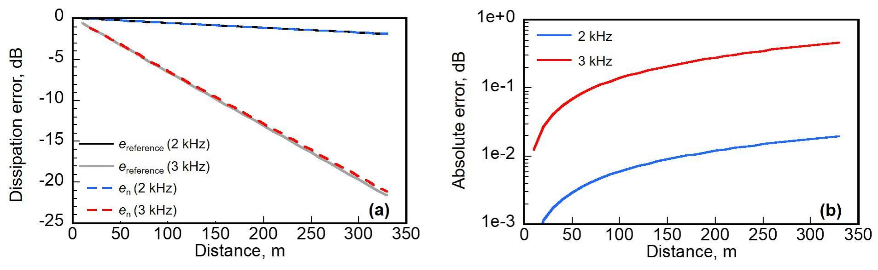
where represents the numerical sound pressure level at point x m apart from the source. Then the numerically calculated error was compared with the theoretically evaluated dissipation error by Equation (41) as shown below.
Figure 7a,b respectively present comparisons of dissipation error between and and absolute errors between and . The results demonstrate that theoretically estimated values have good agreement with the numerical values. As in Figure 7b the discrepancy increases at larger propagation distances and at higher frequencies. This increase is attributable to the contribution of truncated higher order terms in on theoretical analysis. However, the theoretical estimation gives acceptable accuracy with maximum absolute error below 0.5 dB. As the results above showed, one can assess a recommended time interval value easily using Equation (41) in advance.
5. Numerical Experiments with Practical Sound Fields
We demonstrate the performance of the proposed explicit TD-FEM using a modified Adams method via two room acoustic problems at kilohertz frequencies in a large rectangular room including complicated sound diffusers, and in a concert hall with two conditions. The two sound fields have no analytical solution. Therefore, we used a reference solution calculated using well-developed fourth-order accurate implicit TD-FEM [19] to assess the performance. In addition, the performance is shown in comparison to a standard second-order accurate implicit TD-FEM using a Newmark method.
5.1. Standard Implicit TD-FEM and Dispersion Reducing Implicit TD-FEM
Standard implicit TD-FEM solves the second-order ODE of Equation (3) with a time integration method called constant averaged acceleration method: CAA. Actually, CAA is known to be an unconditionally stable Newmark method with parameter . With the space discretization using linear quadrilateral FEs, the resulting implicit time marching scheme has second-order accuracy in both space and time. The implicit time marching scheme is expressed as
where
A Conjugate Gradient (CG) iterative solver is useful to solve a linear system of equations of Equation (45) easily with convergence tolerance of 10. The simplest diagonal scaling is used as a preconditioning technique to facilitate the convergence of an iterative solver. The main operation of standard implicit TD-FEM at each time step comprises sparse MVPs at each iteration process of CG solver and an additional two MVPs. Fourth-order accurate implicit TD-FEM [19,31] for calculating the reference solution also solves the second-order ODE of Equation (3). However, it uses linear quadrilateral FEs with modified integration rules and a highly accurate Newmark method called Fox–Goodwin method. The main operation is the same as standard implicit TD-FEM, but the convergence of iterative solver becomes much better because of the additional effect of modified integration rules. The theoretically estimated dispersion error presented in earlier reports [19,31] shows that this dispersion-reducing implicit TD-FEM has a lower error magnitude than the proposed explicit TD-FEM.
5.2. Sound Propagation Problem in a Rectangular Room Including Acoustic Diffusers
Figure 8a shows the analyzed rectangular room of 10.2 m × 10.8 m surrounded by rigid boundaries with a source point and 27 receivers. The acoustic diffuser, which includes eight periods with a period of 1.2 m, is installed periodically in front of a wall with air spaces. Figure 8b presents details of diffusers. This room cannot be modeled with staircase approximation unless one uses very small rectangular elements because the diffusers comprise rigid reflectors of 0.25 m thickness inclined at various angles against the back wall. However, the proposed explicit TD-FEM can fit the inclined boundaries with fewer elements because of discretization using irregularly shaped FEs. We discretized this room using the irregular FEs with 0.017 m maximum edge length, which corresponds to 6.74 PPW at 3 kHz. The discretization result around the diffusers is shown in Figure 8c. The degrees of freedom (DOF) in this problem are 552,054. As a sound source signal, the Gaussian pulse with the upper-limit frequency of 3 kHz was used. The sound pressure waveforms were calculated at 27 receivers up to 0.1 s with the time interval of 1/120,000 s, which was determined from Equation (38) with the minimum edge length of used mesh. For the standard implicit TD-FEM, the same mesh and time interval were applied. Regarding the measurement accuracy, we use the relative error in sound pressure at each receiver between the reference solution and numerical solution as
where represents the total number of computed time steps. Also, and respectively denote the reference solution and numerical sound pressure at i–th time step. Regarding the calculation of reference solution, sufficiently fine mesh of 15.3 PPW at 3 kHz was used.
Results and Discussion
First, a comparison of sound propagation among the reference solution, the proposed explicit TD-FEM, and the standard implicit TD-FEM are portrayed in Figure 9, where the results at t = 16, 32, and 64 ms are presented. The sound propagation properties of proposed explicit TD-FEM agree very well with the reference solution. It shows an isotropic and less dispersive sound propagation. In contrast, the standard implicit TD-FEM shows a dispersive and an anisotropic sound propagation, where the sound speed in axial directions is faster than those in oblique directions. This result in sound interference occurs at an earlier time, as in the result at 32 ms. Additionally, the wavefront becomes indistinct at later than 64 ms.
Figure 10 presents comparisons of sound pressure waveforms at a receiver (x, y) = (5.3, 3.0) among the reference solution, the proposed explicit TD-FEM, and the standard implicit TD-FEM. The proposed explicit TD-FEM shows much better agreement with the reference solution, but it includes slight difference in amplitude. This agreement confirms that the proposed explicit TD-FEM has superior performance for dealing with discretization of sound fields including complex geometries. However, the standard implicit TD-FEM shows marked discrepancy from the reference solution because of the large dispersion error. As described, the effect appears as an increase of sound speed. The effects are visible even in the direct sound. Moreover, they accumulate with time. Additionally, one can observe that the standard implicit TD-FEM cannot capture reflected waves with high amplitude accurately at around t = 0.06 and 0.07 s. More quantitatively, regarding spatial averaged relative errors, the proposed explicit TD-FEM has one-third lower relative error of 0.316% compared to the error 1.031% in standard implicit TD-FEM. In addition, the proposed explicit TD-FEM has other benefits for computational time. The proposed method can compute 4.55 times faster with the total number of MVP of 24,000 in the proposed method and 109,109 in the standard method.
5.3. Sound Propagation in a Concert Hall
A second numerical example demonstrates the performance in a more practical application. Figure 11 presents analyzed concert hall models of 296 m surface area with two conditions. In the figure, Cond. 1 is a basic model; Cond. 2 is a model including an acoustic reflector above the stage and rib structures at a back wall in the stage for sound scattering. The reflector has 5.86 m length with 0.4 m width; the rib structure has a 0.4 m period length with 0.1 m depth and 0.2 m width. We used the simplest equivalent impedance model to address sound absorption effects at boundaries. For the seat and the back wall in the audience area, represented respectively as red and yellow lines in Figure 11, we gave = 3.87 and = 7.14 respectively. They correspond to Paris’s statistical absorption coefficients, , of 0.8 and 0.6, which are calculated as
Other boundaries including the reflector surfaces were set as =71.519 corresponding to = 0.1. As a sound source, we used an impulse response of fourth-order Butterworth type bandpass filter with 1/3 octave band width centered at 2 kHz. The source waveform and its frequency spectrum are portrayed in Figure 12. The band-limited room impulse responses were calculated up to 2 s at 15 receivers R1–R15, as listed in Table 2. The concert hall models were discretized using four-node quadrilateral FEs with maximum edge length of 0.02 m, which corresponded to 7.65 PPW at the upper-limit frequency of 2 kHz 1/3 octave band. The discretized FEM models have 806,478 DOF and 880,796 DOF, respectively, for Cond. 1 and Cond. 2. We set as 1/98,000 s. As for the measure of accuracy, because one important evaluation in room acoustics is conducted using room acoustical parameters such as reverberation time, clarity, and strength, the absolute error in time integrated sound pressure level might become a useful measure. It is defined as shown below.
In that equation, and respectively denote the numerical solution and reference solution at time t. For computing the reference solution, the same FE meshes were used because the theoretically estimated maximum dispersion error of reference method with these meshes is lower than 0.1%.
Results and Discussion
Figure 13 portrays comparisons of direct sound waveforms at R1 (x, y) = (15.1, 1.25) for the reference solution and the proposed explicit TD-FEM and the standard implicit TD-FEM for Cond. 1. Results for Cond. 2 were omitted because similar results were obtained. The proposed explicit TD-FEM shows good agreement with the reference solution, whereas the standard implicit method shows a marked discrepancy with an increased sound speed because of the larger dispersion property. Figure 14 presents a comparison of impulse responses up to 1.0 s for Cond. 1 and Cond. 2. The proposed explicit TD-FEM shows much better agreement with the reference solution in the entire time range for both conditions. However, the standard implicit TD-FEM shows poor approximation capability. In the early time region, it underestimates the amplitude of reflected waves, which is also observed for reflected waves at around 0.4 s for Cond. 1. Figure 15 presents a comparison of absolute error between the proposed method and standard method for Cond. 1 and Cond. 2, where the error is the averaged value for all receivers. It is calculated at the time after arrival of the direct sound. The proposed explicit TD-FEM presents much lower errors for both conditions with magnitude below 0.2 dB. The standard implicit TD-FEM has error magnitude of approximately 0.4 dB and 0.6 dB for Cond. 1 and Cond. 2. In addition, the error level increases for more complicated Cond. 2. Regarding the advantage of using explicit TD-FEM, it can simulate sound propagation in concert halls, with approximately one-fifth less computational time than that of the implicit standard TD-FEM and one-third times the fourth-order accurate implicit TD-FEM used for reference calculation. These results suggest the high efficiency of the proposed explicit TD-FEM for acoustic simulations in complicated sound fields at kilohertz frequencies. For reference, total numbers of MVP required for the respective methods are 392,000 for the proposed explicit method, 1,995,506–2,053,979 for the standard implicit method, and 1,219,622–1,306,921 for the fourth-order implicit method.
Figure 16 presents sound propagation in the concert hall for both conditions calculated using the proposed explicit TD-FEM. It shows again that the sound propagation is isotropic. Additionally, one can observe from the result of Cond. 2 that the effect of increased diffuseness of resulting sound fields can be gained by virtue of the sound scattering by the rib structures. It is also apparent from the effect of the reflector that strong reflection of sound from the reflector comes at an earlier time to the audience area than reflection waves from the ceiling and back wall of the stage. Furthermore, Figure 17 shows time-integrated SPL until 0.1 s for Cond. 1 and Cond. 2. By installing the reflector, it is readily apparent that early incident sound energies on the audience area increase and that sound energies around the back wall of the stage decrease. These results demonstrate the effectiveness of the proposed explicit TD-FEM clearly as a room acoustic design tool in practical applications.
6. Conclusions
The study described in this report examined a proposed time domain room acoustic solver using an explicit TD-FEM and demonstrated its practicality as a room acoustic design tool. The present TD-FEM achieves fourth-order accuracy in both space and time using a dispersion-reduced low-order FEs and a specially designed linear multi-step time integration method. It completely overcomes the shortcomings of earlier presented methods fourth-order accurate explicit formulation [25] by which the staircase approximation is introduced into boundary modeling to maintain higher order accuracy in time discretization. In addition, as a noteworthy feature of the proposed method, it does not necessitate any additional computational cost in the matrix-vector product operations per time step. Therefore, the main operation complexity of the present method is the same as that of an earlier method. We conducted both dispersion and dissipation error analyses of the present method. The dispersion error analysis revealed that the maximum and minimum dispersion errors occur respectively at sound propagation in the axial direction and in an oblique direction = in a polar coordinate system. In addition, the dispersion error decreases with a smaller time interval. The dispersion analysis also revealed that the present method includes a dissipation error that appears as a numerical complex sound speed in the resulting expression. However, we demonstrated that the dissipation error magnitude is dependent only on time interval values. It can simply reduce the control of time interval values using a proposed control method. Performance of the proposed explicit TD-FEM was examined against the standard implicit TD-FEM using sound propagation problems in a concert hall and in a rectangular room including acoustic diffusers. The results clearly demonstrated that the proposed method can predict complex sound fields at kilohertz frequencies accurately with a much lower requirement for computational resources, suggesting its promising potential for use as a time domain room acoustic solver. Although this paper only describes 2D analysis and its results, extension of the proposed method to 3D analysis is a trivial task. It will be a subject of future research.
Author Contributions
Conceptualization, T.Y. and T.O.; Investigation, T.Y.; Methodology, T.Y.; supervision, T.O.; Project administration, K.S.; Validation, T.Y.; Visualization, T.Y.; Writing—Original draft, T.Y and T.O.; Writing—Review & editing, T.Y., T.O. and K.S. All authors have read and agreed to the published version of the manuscript.
Funding
This research received no external funding.
Conflicts of Interest
The authors declare that they have no conflict of interest related to this report or the study it describes.
References
- Sakuma, T.; Sakamoto, S.; Otsuru, T. Introduction. In Computational Simulation in Architectural and Environmental Acoustics—Methods and Applications of Wave-Based Computation; Springer: Tokyo, Japan, 2014; pp. 1–7. [Google Scholar]
- Allred, J.C.; Newhouse, A. Application of the Monte Carlo method to architectural acoustics. J. Acoust. Soc. Am. 1958, 30, 1–3. [Google Scholar] [CrossRef]
- Krokstad, A.; Strom, S.; Sørsdal, S. Calculating the acoustical room response by the use of a ray tracing technique. J. Sound Vib. 1968, 8, 118–125. [Google Scholar]
- Vorländer, M. Simulation of sound in rooms. In Auralization: Fundamentals of Acoustics, Modelling, Simulation, Algorithms and Acoustic Virtual Reality; Springer Science & Business Media: Berlin/Heidelberg, Germany, 2007; pp. 175–226. [Google Scholar]
- Savioja, L.; Svensson, U.P. Overview of geometrical room acoustic modeling techniques. J. Acoust. Soc. Am. 2005, 138, 708–730. [Google Scholar] [CrossRef] [PubMed] [Green Version]
- Rindel, J.H.; Nielsen, G.B.; Christensen, C.L. Diffraction around corners and over wide barriers in room acoustic simulations. In Proceedings of the 16th International Congress on Sound and Vibration, Kraków, Poland, 5–9 July 2009. [Google Scholar]
- Rindel, J.H. Computer simulation techniques for acoustical design of rooms. Acoust. Aust. 1995, 23, 81–86. [Google Scholar]
- Botteldooren, D. Finite-difference time-domain simulation of low-frequency room acoustic problems. J. Acoust. Soc. Am. 1995, 98, 3302–3308. [Google Scholar] [CrossRef]
- LoVetri, J.; Mardare, D.; Soulodre, G. Modeling of the seat dip effect using the finite-difference time-domain method. J. Acoust. Soc. Am. 1996, 100, 2204–2212. [Google Scholar] [CrossRef]
- Sakamoto, S. Phase-error analysis of high-order finite difference time-domain scheme and its influence on calculation results of impulse response in closed sound field. Acoust. Sci. Technol. 2007, 28, 295–309. [Google Scholar] [CrossRef] [Green Version]
- Kowalczyk, K.; Van Walstijn, M. Room Acoustics Simulation Using 3-D Compact Explicit FDTD Schemes. IEEE Trans. Audio Speech Lang. Process. 2010, 19, 34–46. [Google Scholar] [CrossRef] [Green Version]
- Hamilton, B.; Bilbao, S. FDTD Methods for 3-D Room Acoustics Simulation with High-Order Accuracy in Space and Time. IEEE Trans. Audio Speech Lang. Process. 2017, 25, 2112–2124. [Google Scholar] [CrossRef]
- Bilbao, S. Modeling of Complex Geometries and Boundary Conditions in Finite Difference/Finite Volume Time Domain Room Acoustics Simulation. IEEE Trans. Audio Speech Lang. Process. 2013, 21, 1524–1533. [Google Scholar]
- Hamilton, B.; Webb, C.J.; Fletcher, N.; Bilbao, S. Finite difference room acoustics simulation with general impedance boundaries and viscothermal losses in air: Parallel implementation on multiple GPUs. In Proceedings of the International Symposium on Musical and Room Acoustics ISMRA 2016, La Plata, Argentine, 11–13 September 2016. [Google Scholar]
- Azad, H.; Siebein, G.W.; Ketabi, R. A Study of Diffusivity in Concert Halls Using Large Scale Acoustic Wave-Based Modeling and Simulation. In Proceedings of the 47th International Congress and Exposition on Noise Control Engineering, Chicago, IL, USA, 26–28 August 2018. [Google Scholar]
- Craggs, A. The transient response of a coupled plate-acoustic system using plate and acoustic finite elements. J. Sound Vib. 1971, 15, 509–528. [Google Scholar] [CrossRef]
- Otsuru, T.; Okamoto, N.; Okuzono, T.; Sueyoshi, T. Applications of large-scale finite element sound field analysis onto room acoustics. In Proceedings of the 19th International Congress on Acoustics, Madrid, Spain, 2–7 September 2007. [Google Scholar]
- Okuzono, T.; Otsuru, T.; Tomiku, R.; Okamoto, N. Fundamental accuracy of time domain finite element method for sound-field analysis of rooms. Appl. Acoust. 2010, 71, 940–946. [Google Scholar] [CrossRef] [Green Version]
- Okuzono, T.; Otsuru, T.; Tomiku, R.; Okamoto, N. Application of modified integration rule to time-domain finite-element acoustic simulation of rooms. J. Acoust. Soc. Am. 2012, 132, 804–813. [Google Scholar] [CrossRef]
- Okuzono, T.; Otsuru, T.; Tomiku, R.; Okamoto, N. A finite-element method using dispersion reduced spline elements for room acoustics simulation. Appl. Acoust. 2014, 79, 1–8. [Google Scholar] [CrossRef] [Green Version]
- Papadakis, N.M.; Stavroulakis, G.E. Effect of Mesh Size for Modeling Impulse Responses of Acoustic Spaces via Finite Element Method in the Time Domain. In Proceedings of the Euronoise 2018, Crete, Greece, 27–31 May 2018. [Google Scholar]
- Okuzono, T.; Sakagami, K.; Osturu, T. Dispersion-reduced time domain FEM for room acoustics simulation. In Proceedings of the 23rd International Congress on Acoustics, Aachen, Germany, 9–13 September 2019. [Google Scholar]
- Newmark, N.M. A method of computation for structural dynamics. J. Eng. Mech. Div. 1959, 85, 67–94. [Google Scholar]
- Okuzono, T.; Yoshida, T.; Sakagami, K.; Otsuru, T. An explicit time-domain finite element method for room acoustics simulations: Comparison of the performance with implicit methods. Appl. Acoust. 2016, 104, 76–84. [Google Scholar] [CrossRef]
- Yoshida, T.; Okuzono, T.; Sakagami, K. Numerically stable explicit time-domain finite element method for room acoustics simulation using an equivalent impedance model. Noise Control Eng. J. 2018, 66, 176–189. [Google Scholar] [CrossRef]
- Yoshida, T.; Okuzono, T.; Sakagami, K. A three-dimensional time-domain finite element method based on first-order ordinary differential equations for treating permeable membrane absorbers. In Proceedings of the 25th International Congress on Sound and Vibration, Hiroshima, Japan, 8–12 July 2018. [Google Scholar]
- Wang, H.; Sihar, I.; Muoz, R.P.; Hornikx, M. Room acoustics modeling in the time-domain with the nodal discontinuous Galerkin method. J. Acoust. Soc. Am. 2019, 145, 2650–2663. [Google Scholar] [CrossRef] [Green Version]
- Pind, F.; Engsig-Karup, A.P.; Jeong, C.H.; Hesthaven, J.S.; Mejling, M.S.; Strømann-Anderson, J. Time domain room acoustic simulations using the spectral element method. J. Acoust. Soc. Am. 2019, 145, 3299–3310. [Google Scholar] [CrossRef] [Green Version]
- Hughes, T.J.R. Formulation of parabolic, hyperbolic, and elliptic-eigenvalue problems. In The Finite Element Method: Linear Static and Dynamic Finite Element Analysis; Dover: New York, NY, USA, 2000; pp. 436–446. [Google Scholar]
- Zienkiewicz, O.C.; Taylor, R.L.; Zhu, J.Z. The time dimension: Semi-discretization of field and dynamic problems. In The Finite Element Method: Its Basis and Fundamentals, 7th ed.; Butterworth-Heinemann: Oxford, UK, 2013; pp. 382–386. [Google Scholar]
- Yue, B.; Guddati, M.N. Dispersion-reducing finite elements for transient acoustics. J. Acoust. Soc. Am. 2005, 118, 2132–2141. [Google Scholar] [CrossRef] [Green Version]
- Scherer, P.O.J. Equations of motion. In Computational Physics: Simulation of Classical and Quantum Systems, 3rd ed.; Springer Nature: Berlin/Heidelberg, Germany, 2017; pp. 306–308. [Google Scholar]
- Von Neumann, J.; Richtmyer, R.D. A method for the numerical calculation of hydrodynamic shocks. J. Appl. Phys. 1950, 21, 232–237. [Google Scholar] [CrossRef]
- Thompson, L.L. A review of finite-element methods for time-harmonic acoustics. J. Acoust. Soc. Am. 2006, 119, 1315–1330. [Google Scholar] [CrossRef] [Green Version]
Figure 1.
Two-dimensional plane wave propagation in a free field under a polar coordinate system discretized by square finite elements (FEs) with element size of h for dispersion analysis.
Figure 1.
Two-dimensional plane wave propagation in a free field under a polar coordinate system discretized by square finite elements (FEs) with element size of h for dispersion analysis.

Figure 2.
Dispersion characteristics of explicit time domain finite element method (TD-FEM) using modified Adams method: (a) anisotropic characteristics in the dispersion error in terms of sound propagation directions with two time interval values of and and (b) convergence of dispersion error relative to spatial resolution points per wavelength (PPW).

Figure 3.
Modulated Gaussian pulse with upper-limit frequency of 2.5 kHz: (a) waveform and (b) frequency characteristics.
Figure 3.
Modulated Gaussian pulse with upper-limit frequency of 2.5 kHz: (a) waveform and (b) frequency characteristics.

Figure 4.
Waveforms at the receivers in the axial direction (upper row) and the diagonal direction (lower row) between the reference solution and the proposed method for three FE meshes (Mesh-1, -2 and -3) listed in Table 1.
Figure 4.
Waveforms at the receivers in the axial direction (upper row) and the diagonal direction (lower row) between the reference solution and the proposed method for three FE meshes (Mesh-1, -2 and -3) listed in Table 1.

Figure 5.
Theoretical dissipation error characteristics of the proposed method: (a) anisotropic characteristics in terms of sound propagation directions at 2 kHz and 3 kHz and (b) convergence of dissipation error relative to time resolution.
Figure 5.
Theoretical dissipation error characteristics of the proposed method: (a) anisotropic characteristics in terms of sound propagation directions at 2 kHz and 3 kHz and (b) convergence of dissipation error relative to time resolution.

Figure 6.
Long numerical duct model with 400 m length.

Figure 7.
Theoretical and numerical dissipation errors: (a) vs. at 2 kHz and 3 kHz and (b) absolute errors from at 2 kHz and 3 kHz.
Figure 7.
Theoretical and numerical dissipation errors: (a) vs. at 2 kHz and 3 kHz and (b) absolute errors from at 2 kHz and 3 kHz.

Figure 8.
(a) Analyzed sound field including acoustic diffuser with a source point and 27 receivers located on a grid of 1.2 m × 1.2 m. (b) Details of installed acoustic diffuser for one period. (c) Details of discretization of the room around the acoustic diffuser.
Figure 8.
(a) Analyzed sound field including acoustic diffuser with a source point and 27 receivers located on a grid of 1.2 m × 1.2 m. (b) Details of installed acoustic diffuser for one period. (c) Details of discretization of the room around the acoustic diffuser.

Figure 9.
Comparison of sound propagations at t = 16, 32, and 64 ms among (a) Reference, (b) the proposed explicit TD-FEM and (c) the standard implicit TD-FEM.
Figure 9.
Comparison of sound propagations at t = 16, 32, and 64 ms among (a) Reference, (b) the proposed explicit TD-FEM and (c) the standard implicit TD-FEM.

Figure 10.
Comparisons of sound pressure waveforms at a receiver (x, y) = (5.3, 3.0) among the reference solution, the proposed explicit TD-FEM, and the standard implicit TD-FEM.
Figure 10.
Comparisons of sound pressure waveforms at a receiver (x, y) = (5.3, 3.0) among the reference solution, the proposed explicit TD-FEM, and the standard implicit TD-FEM.

Figure 11.
Concert hall models of two conditions (Cond. 1 and Cond. 2) where red and yellow lines respectively represent seat zone with = 3.87 and back wall with = 7.14.
Figure 11.
Concert hall models of two conditions (Cond. 1 and Cond. 2) where red and yellow lines respectively represent seat zone with = 3.87 and back wall with = 7.14.

Figure 12.
Source signal of fourth-order Butterworth type 1/3 octave bandpass filter with center frequency of 2 kHz: (a) impulse response and (b) frequency characteristic.
Figure 12.
Source signal of fourth-order Butterworth type 1/3 octave bandpass filter with center frequency of 2 kHz: (a) impulse response and (b) frequency characteristic.

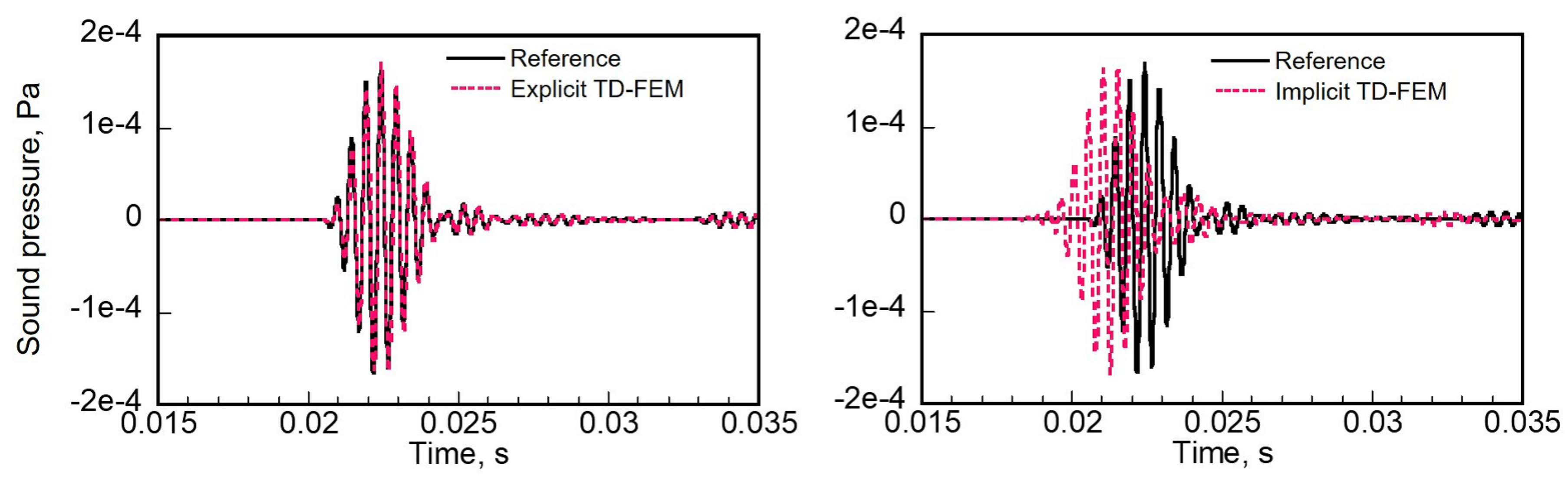
Figure 13.
Comparisons of direct sound waveform at R1: the reference solution vs. the proposed explicit TD-FEM (Left) and the reference solution vs. the standard implicit TD-FEM (right).
Figure 13.
Comparisons of direct sound waveform at R1: the reference solution vs. the proposed explicit TD-FEM (Left) and the reference solution vs. the standard implicit TD-FEM (right).

Figure 14.
Band-limited impulse responses at R1 among the reference solution, the proposed explicit TD-FEM, and the standard implicit TD-FEM for Cond. 1 (upper row) and Cond. 2 (lower row).
Figure 14.
Band-limited impulse responses at R1 among the reference solution, the proposed explicit TD-FEM, and the standard implicit TD-FEM for Cond. 1 (upper row) and Cond. 2 (lower row).

Figure 15.
Comparison of absolute errors in time integrated sound pressure levels between the proposed explicit TD-FEM and the standard implicit TD-FEM for Cond. 1 and Cond. 2.
Figure 15.
Comparison of absolute errors in time integrated sound pressure levels between the proposed explicit TD-FEM and the standard implicit TD-FEM for Cond. 1 and Cond. 2.

Figure 16.
Sound propagation in a concert hall model for Cond. 1 (left column) and Cond. 2 (right column) at t = 10, 30 and 50 ms.
Figure 16.
Sound propagation in a concert hall model for Cond. 1 (left column) and Cond. 2 (right column) at t = 10, 30 and 50 ms.

Figure 17.
Comparison of time-integrated sound pressure level until 0.1 s for Cond. 1 (upper) and Cond. 2 (lower).
Figure 17.
Comparison of time-integrated sound pressure level until 0.1 s for Cond. 1 (upper) and Cond. 2 (lower).


Table 1.
Details of three FE meshes (Mesh-1, -2 and -3) for convergence test: h and PPW respectively denote the length of square FE and the number of points per wavelength.
Table 1.
Details of three FE meshes (Mesh-1, -2 and -3) for convergence test: h and PPW respectively denote the length of square FE and the number of points per wavelength.
| Mesh | h, m | PPW |
|---|---|---|
| Mesh-1 | 0.02 | 6.87 |
| Mesh-2 | 0.01 | 13.75 |
| Mesh-3 | 0.005 | 27.45 |
Table 2.
List for 15 receiver positions (R1–R15) in concert hall model.
| Receiver | (x, y), m | Receiver | (x, y), m |
|---|---|---|---|
| R1 | (15.1, 1.25) | R9 | (6.3, 3.5) |
| R2 | (14.1, 1.5) | R10 | (5.3, 3.9) |
| R3 | (13.1, 1.7) | R11 | (4.3, 4.3) |
| R4 | (12.1, 2.0) | R12 | (3.3, 4.7) |
| R5 | (11.1, 2.1) | R13 | (2.3, 5.1) |
| R6 | (10.1, 2.5) | R14 | (1.3, 6.3) |
| R7 | (8.3, 2.7) | R15 | (0.8, 6.7) |
| R8 | (7.3, 3.1) |
© 2020 by the authors. Licensee MDPI, Basel, Switzerland. This article is an open access article distributed under the terms and conditions of the Creative Commons Attribution (CC BY) license (http://creativecommons.org/licenses/by/4.0/).
Share and Cite
MDPI and ACS Style
Yoshida, T.; Okuzono, T.; Sakagami, K. Time Domain Room Acoustic Solver with Fourth-Order Explicit FEM Using Modified Time Integration. Appl. Sci. 2020, 10, 3750. https://doi.org/10.3390/app10113750
AMA Style
Yoshida T, Okuzono T, Sakagami K. Time Domain Room Acoustic Solver with Fourth-Order Explicit FEM Using Modified Time Integration. Applied Sciences. 2020; 10(11):3750. https://doi.org/10.3390/app10113750
Chicago/Turabian StyleYoshida, Takumi, Takeshi Okuzono, and Kimihiro Sakagami. 2020. "Time Domain Room Acoustic Solver with Fourth-Order Explicit FEM Using Modified Time Integration" Applied Sciences 10, no. 11: 3750. https://doi.org/10.3390/app10113750
Note that from the first issue of 2016, this journal uses article numbers instead of page numbers. See further details here.