Optimization of the Schedule for the Whole Process in Hot Strip Manufacturing
by
 ,
,
Wen Peng
1, 
Jianyang Ma
1,
Xiaorui Chen
1,
Yafeng Ji
2,
Jie Sun
1,
Jinggou Ding
1 and
Dianhua Zhang
1,* 1
State Key Laboratory of Rolling and Automation, Northeastern University, Shenyang 110819, China
2
School of Mechanical Engineering, Taiyuan University of Science and Technology, Taiyuan 030024, China
*
Author to whom correspondence should be addressed.
Metals 2020, 10(6), 717; https://doi.org/10.3390/met10060717
Submission received: 26 April 2020
/
Revised: 22 May 2020
/
Accepted: 27 May 2020
/
Published: 28 May 2020
Abstract
:Optimization of the schedule is an effective way to reduce energy consumption in hot strip manufacturing. The heating energy and the rolling energy contribute the vast majority of the energy consumption. In order to reduce the energy consumption for the whole process, an optimization method based on the multi-objective function was applied, and the heating energy and rolling energy were both taken into consideration during the function modeling. Meanwhile, process constraints and equipment limitations were taken as objective function boundary conditions, and the tapping temperature in the furnace exit and thickness of each pass were decision variables. Further, to obtain the optimal solution of the objective function, the differential evolution algorithm was used, finally, the optimal tapping temperature and the thickness were obtained successfully. Meanwhile, the validity of the calculated results was verified by comparing with the actual process in a hot rolling production line in Hebei province, the results indicated that with the proposed method, a more reasonable schedule were obtained; compared with the existing actual schedule of typical specification, the energy consumption can be reduced by about 1.5%.
1. Introduction
The manufacturing process of the hot-rolled strip is a complex industrial process covering multiple procedures and multiple control levels, and it is effective support for the development of national economy [1]. Currently, energy saving and emission reduction have become the focus of attention in the iron and steel industry, especially in the hot rolling process. A series of energy saving technologies has been applied to the manufacturing of the hot-rolled strip in new building plants, like continuous casting technology, hot transportation and hot charging and direct rolling of continuous casting ingot and combustion technology in heating consumption [2]. For early plants, the aforementioned production equipment and technology cannot be implemented effectively, because of the transformation cost and production layout constraints, in order to reduce the energy consumption, the schedule adjustment and optimization should be given more attention.
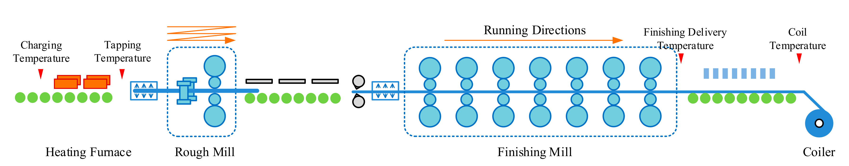
Figure 1 shows the layout of the typical hot rolling line, which includes the heating furnace, rough mill and the finishing mill. The initial slab is heated to the tapping temperature in the heating furnace, and the final production with regular shapes is obtained by reciprocating rolling in rough mill and continuous rolling in finishing mill. For the whole process of production, the heating energy of heating furnace and the rolling energy of the mills contribute most of the energy consumption.
How to obtain the target tapping temperature at minimum fuel consumption is a key discussion in heating consumption reduction, as the heat treatment equipment is necessary in the hot rolling line [3]. Steinboeck [4] analyzed the radiant heat transfer system, and the heat flow state on surface and temperature distribution inside were predicted based on the proposed heat transfer model. The heating furnace was simulated as a radiating medium with temperature spatial variation and constant absorption coefficient by Kim [5,6]. In Miao’s study [7], the effectiveness and accuracy of transient heat flow prediction on the surface of the billets were verified by an actual case. Suzuki [8] proposed a simulation method to optimize billets layout and internal heat control simultaneously. Emadi [9] simulated the heating characteristics of billets by developing a mathematical heat transfer model, and the weighted-sum-of-gray-gas-model was used for gas radiation prediction; also, the convective heat flux was calculated by considering suitable value of convective heat transfer coefficient at any location of the furnace. In Morgado’s numerical model [10], the turbulent reaction flow in the furnace, the heat conduction and the periodic motion of walking beam were simulated. Han [11] predicted the transient radiative heating characteristics of billets by the radiation finite volume method, and the motion of the billets was taken into consideration, and the heating characteristics of the billets at different temperatures were also analyzed. Casal [12] proposed a new method for CFD 3-dimensional simulation of a walking-beam type reheating furnace in steady state; in his study, the movement of billets was performed by modifying the energy transport equation, and the method can reduce the calculation time compared with the transient modeling method. Depree [13] studied the temperature distribution by means of a three-dimensional model built by COMSOL; the measured data obtained by thermocouple was used to improve the temperature prediction accuracy of the furnace and billets. The long computation time limits the further online application of the CFD method, and the uncertainty and nonlinearity of the actual industrial conditions in industrial settings also limit the application of the mentioned simulation technology. In order to solve practical engineering problems, a series of intelligent control technologies for heating furnaces were proposed. Feliu [14] proposed a simple fractional order controller, combined with a Smith predictor scheme for temperature controlling in the reheating furnace. The dynamic model of the preheating zone was obtained from an identification program. Wang [15] discussed the balanced heating, rapid heating and uniform heating schedule, and the adaptability of the heating furnace to different heating processes was also analyzed. In order to calculate the production process precisely, the artificial intelligence and artificial neural networks was used to increase the heating efficiency, Wang [16] proposed an improved method integrated with the parameter-adaptive mnemonic enhancement optimization method (AMEO-CNN) to describe the heating process, and the thermal efficiency of the furnace was improved. Prieler [17] used the neural network to describe the temperature distribution in a furnace in dependence of the process parameters, in which a novel CFD was used to investigate and improve the process. The multi-objective genetic algorithm was used to optimize the temperature distribution. Thanks to their effective research work, for certain tapping temperatures, we were able to achieve precise control of the tapping temperature at the required fuel consumption.
Similarly, lots of effective work on reducing rolling energy had been proposed. How to determine the rolling schedule with the lowest rolling energy has become a major research topic for the rolling process. During the rough rolling, the comprehensive equal essential load distribution method and the equal load function method were used to distribute the loading of each pass [18]. In more plants, the empirical method was still used, in which the rolling schedule was designed by the operator, and different distribution results were obtained by different operators, and the rolling schedule was stored in series of tables for invocation, and the thickness distribution should be adjusted after instability occurs. For the finishing rolling process, besides the energy consumption curve method, the single objective optimization method and the multi-objective optimization method were used to obtain the required schedules. The energy consumption curve method was one typical empirical method—the key of this approach is to draw the relationship curve between the energy consumption and the thickness by the history of the energy consumption data—then, the loading distribution was obtained, based on the required ratio. In these methods, a large number of field measurement and empirical data were necessary, and the curves should be updated when the production environment changed. As the speed of computation increases, obtaining the optimal solution of the objective function became another effective way to obtain the rolling schedule. In the design process of the single objective function, not only can the process parameters—like rolling force, finishing delivery temperature, the power and the energy consumption—be taken as final optimization objects, but quality indicators like straightness and thermal crown [19,20,21] can also been considered separately. With the increase of people’s attention to the rolling process, it is difficult for a single objective function to satisfy the requirements of the control process. The multi-objective optimization method has been frequently investigated in recent years, and this method is usually a combination of single-objective optimization functions with a weight distribution coefficient. Some researchers focus on the composition of the multi-objective function. In Jia’s [22] multi-objective load distribution model, the rolling force margin balance, roll wear ratio and strip shape control were taken into account. Other researchers conducted their research from the perspective of weight distribution coefficient. In Li’s [23] function, the profile and rolling energy consumption are selected as objective functions of rolling schedule optimization. In Li’s [24] functions, the rolling power minimization, roll force balance and good strip shape was taken into consideration. Qi [25] took relatively equal load of rolling power and good shape as objective functions, established the optimization mathematical models of the finishing rolling schedule. Han [26] Solved the sheet-strip sequencing problem, which involves sorting the strips in each rolling-turn, with the objective of minimizing the maximal changes in thickness between adjacent sheet-strips and the change times of the thickness, so as to ensure the production of high quality sheet-strips.
From the short review above, we can see that more attention has been focused on single process, whereas the relative work has not yet been carried out for whole process. In other industries, like the pharmaceutical industry or the petrochemical industry, the consideration of two or more process steps has been done in the past, and good optimization results have been obtained, which provides a good reference for the hot rolling production process. The heating process and rolling process are interrelated and interact with each other, so the obtained schedule should not be a local optimal solution of single process. Therefore, in this paper, from the perspective of the whole process, under the premise of considering the limitations of the production process and equipment, an optimal schedule of the whole process was obtained by minimizing the multi-objective function, in which the function was designed to describe the total energy. This includes the heating energy and the rolling energy, and the differential evolution algorithm was applied to find the optimal solutions for the function. The following sections describe the execution of this method, including the modeling of energy consumption objective function, the optimization algorithm and calculation procedure and analysis and discussion.
2. Modeling of Energy Multi-Objective Function
2.1. Multi-Objective Function Design
The multi-objective function is the summation of two single-objective functions, which is given by
where is the heating energy consumption; is the drive motors energy consumption; is the total pass number, , is the pass number of rough rolling, is the pass number of finishing rolling.
For a traditional hot rolling production line, the initial slab thickness and the production final thickness are fixed in the optimization of the rolling schedule. Therefore, in our present work, the variables selected to be optimized through minimization objective function are the tapping temperature and the thicknesses of each pass, and the total number equals to . After determining the values of tapping temperature and the inter-pass thicknesses, the parameters involved in the multi-objective function, such as energy consumption, can be calculated by the models in Section 2.2.
2.2. Mathematical Models
2.2.1. Heating Energy Objective Function
In order to obtain the heating energy, for certain slabs/strip, some necessary assumptions need to be mentioned: 1) the hot charging temperature can be represented by a certain temperature value, which was evenly distributed on the whole slab; 2) the influence of tapping temperature change on thermal regulation can be ignored; 3) the tapping temperature is evenly distributed on the whole slab; 4) an energy conversion coefficient describes the combustion efficiency of the heating furnace.
Based on the above assumptions, the heating energy consumption model can be described as:
where is the mass of the slab; is the specific heat capacity; is the hot charging temperature; is the tapping temperature; is the energy conversion efficiency coefficient.
2.2.2. Rolling Energy Objective Function
The rolling energy comes from the motor that drives the roll to rotate, it can be described as:
where N is the motor rolling power; t is the rolling time during the strip through the roll, s;
The rolling power can be given as:
where M is the rolling torque, kN·m, nr is the motor speed, rad/min;
The rolling torque can be given as:
where is the rolling force, kN; is the arm coefficient, mm; is the contact arc length, mm; contains the additional torque like friction torque, dynamic torque and idling torque.
The SIMS model was used to calculate the rolling force [27]:
where B is the strip width, mm; Qp is the influence coefficient of stress state; KT is the influence coefficient of tension; K is the deformation resistance, K = 1.15σs, MPa;
Deformation resistance is not only related to the chemical composition of materials, it also depends on the physical conditions of plastic deformation, such as deformation temperature, deformation speed and deformation degree, and the typical formula of deformation resistance generally adopts the following type:
where is the basic deformation resistance, MPa; is the deformation temperature, K; is the true strain; is the deformation velocity, s−1;
The influence coefficient of stress state model was defined as:
The total energy calculation is shown in Figure 2.
2.2.3. Temperature Model
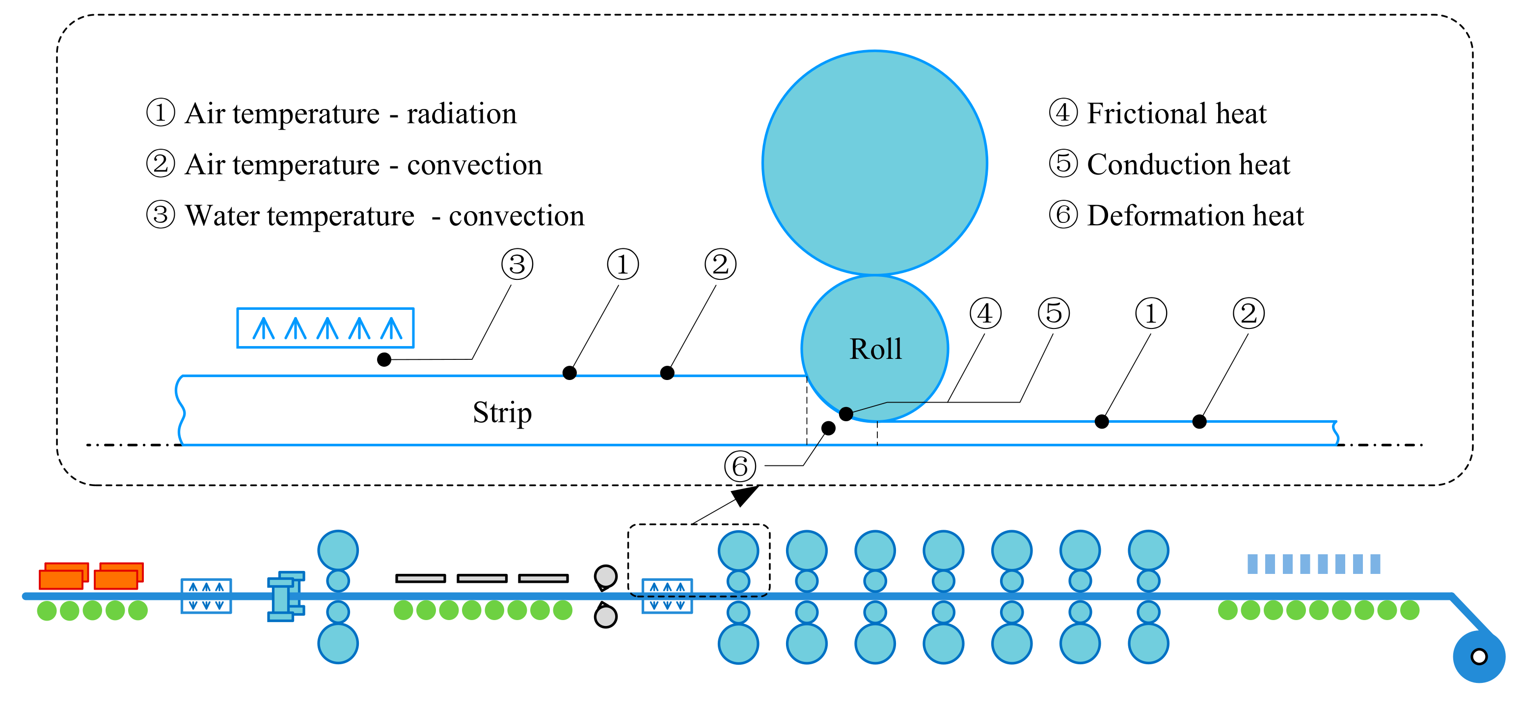
An accurate temperature prediction is a prerequisite for calculating the deformation resistance of rolled slabs, as known to all, the strip temperature changes at any time during the transportation, it experienced air-cooling zone, water-cooling zone and deformation zone, and the temperature of each pass was required to calculate in turn. Figure 3 shows the heat flows during the coil transportation.
The temperature of pass is relative to the deformation resistance in Equation (9), and it can be described as.
where is the temperature change caused by ambient; is the temperature change caused by cooling water; is the temperature change caused by deformation; is the temperature change caused by friction; is the temperature change caused by conduction.
The temperature model contains the air-cooling model, water-cooling model and the deformation zone temperature model.
(1) Air-Cooling Model
During the rolling process, the high-temperature strip loses heat to the surroundings by thermal radiation and heat convection. The literature [28] points that hot loss caused by the heat convection accounts for 5%–7% of the total heat loss, so the effect of thermal convection can be expressed as equivalent emissivity in thermal radiation. The thermal radiation can be described by the Stephen Boltzmann-law, and the final air-cooling model can be described as:
where is the equivalent emissivity; is the density of the strip.
(2) Water-Cooling Model
Water-cooled convection is another type of strip heat transfer that, like the high pressure descaling water and inter-stand water, as a forced convection heat transfer, is difficult to calculate the effect of fluid status (like flow rate, water pressure) theoretically. We used the forced convection heat transfer coefficient to describe the comprehensive influence, and the final water-cooling model can be described as:
where is the forced convection heat transfer coefficient; is the heat transfer time, s.
(3) Deformation Zone Temperature Model
In the deformation zone, there are two contradictory processes in the rolling deformation zone: one is the heat generated by the plastic deformation of the rolling strip, the other is the heat lost by the contact between the high temperature strip and the low temperature work rolls. Additionally, the surface friction heat caused by the relative motion between the rolls and the strip contribute some heat. The final heat is a summation of the change, due to the temperature gained from the deformation energy applied to the piece and the heat flow from the piece to the work rolls.
(1) Deformation Heat Model
The deformation heat generates during the plastic deformation process, which makes the strip temperature rise. The deformation heat model was expressed as:
where is deformation efficiency coefficient;
(2) Friction Heat Model
The friction heat originates from the speed difference between the work roll and the strip, which causes the strip temperature rise, the friction heat model was expressed as:
where is the friction efficiency coefficient; is friction coefficient; is speed difference.
(3) Conduction Heat Model
The conduction heat generated from the temperature difference between the strip and the work roll, the contact heat model was expressed as:
where is the roll contact heat flow coefficient; is strip heat conduction coefficient; is work roll temperature.
2.3. Constraints Conditions
Necessary protection should be provided to ensure equipment safety and production stability, and the constraints and limitation conditions should be taken into account the objective function. In our work, the following process requirements constraints and equipment capacity should be considered.
2.3.1. Process Requirements Constraints
(1) Temperature Constraints
In the hot rolling process, the temperature was important for the internal performance of the product final production. Here, the tapping temperature and the finishing delivery temperature (FDT) should meet the process requirements strictly. A higher tapping temperature means more oxidation loss; a lower tapping temperature means lower finishing delivery temperature, without the help of the heating device. Therefore, for specified production, the tapping temperature was limited to a certain range:
The finishing delivery temperature has a great influence on the metallographic structure and grain size, which has a great influence on its mechanical properties. As a result, they were limited to a certain range, and the finishing delivery temperature constraints were considered:
(2) Thickness Constraints
When the strip is compressed to a certain thickness, it is impossible to make the product thinner due to the elastic flattening of the roll, so the certain thickness was called the minimum reliable thickness [29], and the delivery side thickness of each stand/pass should meet the following condition:
where is the minimum reliable thickness, mm. it can be expressed as:
where is the diameter of the work roll, mm.
Further, for each pass, the entrance thickness should greater than the delivery thickness, the following constraints should also be met.
(3) Reduction Limits Constraints
The maximum reduction of each stand should be kept inside the defined reduction limits, and the bite angle was used to determine whether the smooth bite can be realized in the roll gap, and the reasonable bite conditions ensure the steadiness of the strip threading, and based on the result of the force analysis in bite process, the following relationship should be satisfied,
where is the bite angle, ; is the reduction; is the friction angle; is the friction coefficient, .
(4) Additional Constraints
In order to meet the final strip quality requirements, additional constraints should be taken into consideration. For example, the rolling force of the last stand should maintain the optimal shape to ensure good shape conditions, and such constraints also need to be met.
2.3.2. Equipment Capacity Constraint
(1) Hydraulic Device Constraints
The maximum rolling force has a limiting to protect the hydraulic device,
where is the maximum rolling force the hydraulic device can provide.
(2) Motor Constraint
When the motor outputs the rolling power, it can also drive the work roll by reducer, though the maximum rolling power, torque and rotational speed has a limitation to protect the motor,
where , is the maximum rolling power and torque the motors can provide, is the maximum rotational speed, and can be translated into the velocity constraint of the rolling strip further.
3. Optimization Algorithm and Calculation Procedure
3.1. Differential Evolution Algorithm
As an effective method to solve the optimization problems, the Differential Evolution algorithm (DE) was first put forward by Storn and Price [30]. It is a population-based algorithm that uses mutation, crossover and selection operators. Different from the traditional evolutionary algorithm, the proportional difference vector generated by randomly selected individuals is used to perturb the current generation population, so it is unnecessary to use a separate probability distribution to generate sub-generations. Three important parameters of the algorithm are population size (NP), crossover rate (CR) and scaling factor (F).
The DE algorithm is initialized with NP randomly generated D-dimensional parameter vectors, which indicate candidate solutions for the optimization problems. Then mutation, crossover and selection operations are applied to the individuals to obtain the optimal result, and the process continues until the termination condition is reached.
Let t = 0, 1, 2, 3, …, tmax indicate the next generations; the ith individual of the present generation is expressed as follows:
(1) Mutation Operation
In the DE algorithm, the mutant vector is generated by using a mutation operator for each in each generation. The researchers have proposed different approaches to generate the mutant vector, the following equations showed the vector.
Usually, the mode of the mutant vector was DE/x/y/z, x was chosen in ”rand”, ”best” or ”rand-to-best”, the y was the number of the vector, “1” or ”2” were selected, z was the “binomial cross” or “exponential cross” strategy [31]. Accordingly, the differential update strategy used to generate the mutant vector are shown in Equations (26)–(34).
1. DE/rand/1
2. DE/best/1
3. DE/rand/2
4. DE/best/2
5. DE/current-to-best/1
6. DE/current-to-rand/1
7. DE/rand-to-best/2
8. DE/current-to-rand/1
9. DE/rand-to-best/2
where are random individuals selected from the population, is the best individual of the present population, is a scaling factor that determines how far the search operation will be performed.
(2) Crossover Operation
For each pair of mutant vectors and its related target vector . Therefore, the trial vector can be obtained in accordance with the following:
where is the mutant vectors, is the target vector, is the crossover rate, , is the population size.
(3) Selection Operation
The selection operation determines whether the trial vector or target vector is used. The former is transferred to the next generation if it has a better fitness value than the target vector.
3.2. Calculation Procedure
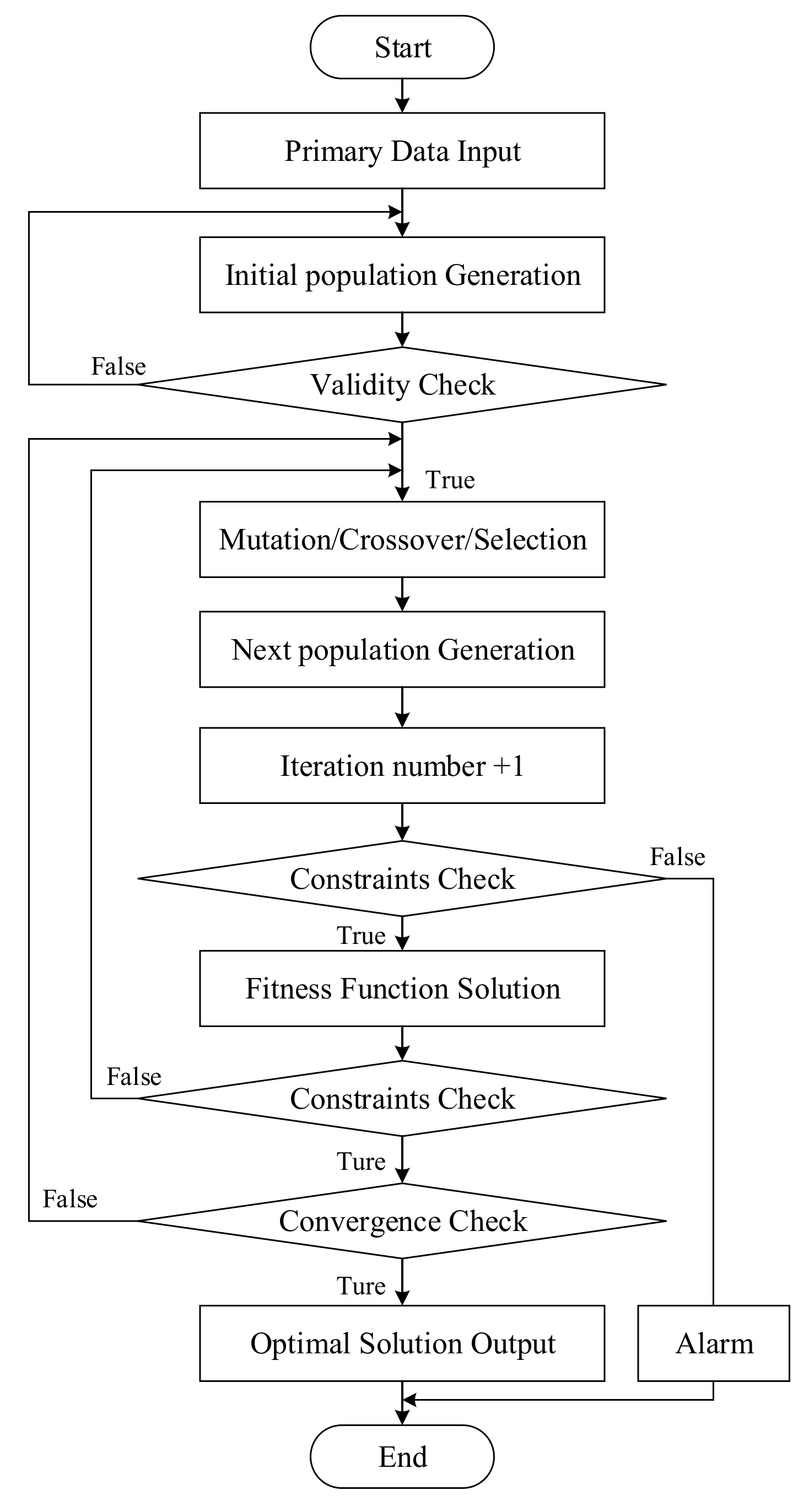
The energy consumption objective function and the solution method were both programmed by C++ language, and the flow chart is shown in Figure 4, which can be explained as follows.
Step 1: according to the primary data of the given production plan, the tapping temperature and the thickness of each pass are initialized as the initial population generation. Meanwhile, the fitness function (objective function), the cross-probability constant, scaling factor and maximum iteration number should be initialized.
Step 2: generate the initial populations by the primary data. The initial population can be obtained from the historical production data, which were validated by actual production, and the total population should meet the quantitative requirements.
Step 3: calculate the fitness function of the initial population, and constraint and limitation conditions checking is carried out. If these are acceptable, go to Step 4, otherwise, go back to Step 2.
Step 4: generate the new populations by mutation and crossover operation, obtain the next population by selection operation, calculate the fitness function and update the iteration number.
Step 5: check the constraint conditions and the iteration number. If these are acceptable, compare them with the current optimal result. If they are better, go to Step 6, otherwise, go back to Step 4.
Step 6: output the optimal solution, stop the iteration.
4. Analysis and Discussion
4.1. Plant Description
In order to verify our present work, data of one 1580 mm hot tandem line in Hebei province of China was used. The line includes one rough mill and seven finishing mills. Each stand is equipped with two single cylinders mounted on the top of stand, which can perform the regulation of the roll gap either in position or in force. Meanwhile, each stand is driven by AC motor, which is mechanically linked to the work rolls in order to control the roll revolution speed.
The tandem mill can reduce the strip from the initial slab thickness 200–220 mm to 1.2–12.7 mm strips, and the coil width range is 700−1450 mm, the maximum coil weight was 28 t, the rolled products mainly consist of carbon steel, low alloy steel, electrical steel and pipe-line steel, etc. The main mechanical and electrical parameters are presented in Table 1.
One coil was randomly selected from coils processed by the tandem mill, the material was Q235B steel (C: 0.12%), the slab size was 200 mm × 1200 mm × 7000 mm (thickness × width × length), the final production size was 2.00mm × 1200mm (thickness × width), the hot charging temperature was 600 °C, and its deformation resistance is determined by Shida’s model [32]. The model regression coefficient is shown in Table 2.
The range of the tapping temperature was 1170−1210 °C, the delivery temperature should not be lower than 860 °C and the other process requirements constraints are presented in Table 3.
The rolling schedule of Q235 steel used in actual production process was shown in Table 4.
4.2. Analysis and Discussion
4.2.1. Analysis of Single Objective Function
In this section, the heating energy and the rolling energy mentioned in Chapter 2.2 were discussed. From Equation (2), the difference between the charging temperature and tapping temperature contributes high proportion of heating energy, as shown in Figure 5, the heating energy increases linearly as the tapping temperature rises, and it also decreases linearly with the rise of the initial temperature. For the heating process, the higher charging temperature and lower tapping means lower heating energy.
It is worth noting that the tapping temperature not only influences the heating energy, it also influences the rolling energy. When the tapping temperature changed, the heating energy and the rolling energy changed simultaneously. For example, under the rolling schedule shown in Table 4, the charging temperature was 600 °C. The composition of the total energy and the proportion of heating energy are shown in Figure 6. It can be seen that, as the tapping temperature rose from 1170 °C to 1210 °C, the proportion of the heating energy rose from 67.1% to 71.7%, and the rolling energy was reduced gradually.
4.2.2. Analysis of Multi-Objective Function
In this section, the multi-objective function was solved by the DE method, in which the tapping temperature and the thickness of each pass were both taken as the optimization factors. Meanwhile, the schedule was obtained by minimizing the multi-objective function, and the actual schedule was participated in comparative verification.
As we know, the tapping temperature was between 1170 °C and 1210 °C. In order to illustrate the change of the total energy consumption, the tapping temperature change step was set as 2.5 °C. for each tapping temperature, the heating energy was calculated by Equation (2), and two different methods were used to calculated the rolling energy. One used the schedule mentioned in Table 4 (first method), and in the second method, the rolling energy was obtained by minimizing the rolling objective function with the DE method (second schedule). The total energy in each tapping temperature are shown in Figure 6. It can be seen that at each tapping temperature, the total energy obtained by the second method was lower than the first method, and the reduced energy percentage grew from 1.18% to 1.38%. This means that, for a certain tapping temperature, the total rolling energy can reach a lower level by minimizing the rolling objective function, and, in Figure 7, when the tapping temperature was 1180 °C, the total energy was lowest (8.2891 × 10⁶ kJ).
In other words, if the tapping temperature change step get smaller, a lower total energy may exist, and it was certain that, for a certain tapping temperature, a desired schedule with the lowest rolling energy can obtained by minimizing the rolling objective function. Further, an optimized schedule with the lowest total energy may exist in the tapping temperature between 1170 and 1210 °C.
Furthermore, by minimizing the multi-objective function mentioned in Equation (1), we obtained the final schedule, and the tapping temperature and the thickness of each pass were optimized simultaneously. Figure 8 shows a comparison of the heating energy, rolling energy and total energy of three schedules. In addition to the actual schedule with a tapping temperature of 1180 °C (Schedule 1 in Figure 8), the schedule obtained by minimizing the rolling objection function with tapping temperature 1180 °C (Schedule 2 in Figure 8) is also shown. The tapping temperature of the schedule by minimizing the multi-objective function is 1181.9 °C (Schedule 3 in Figure 8), and the details of these three schedules are shown in Table 5.
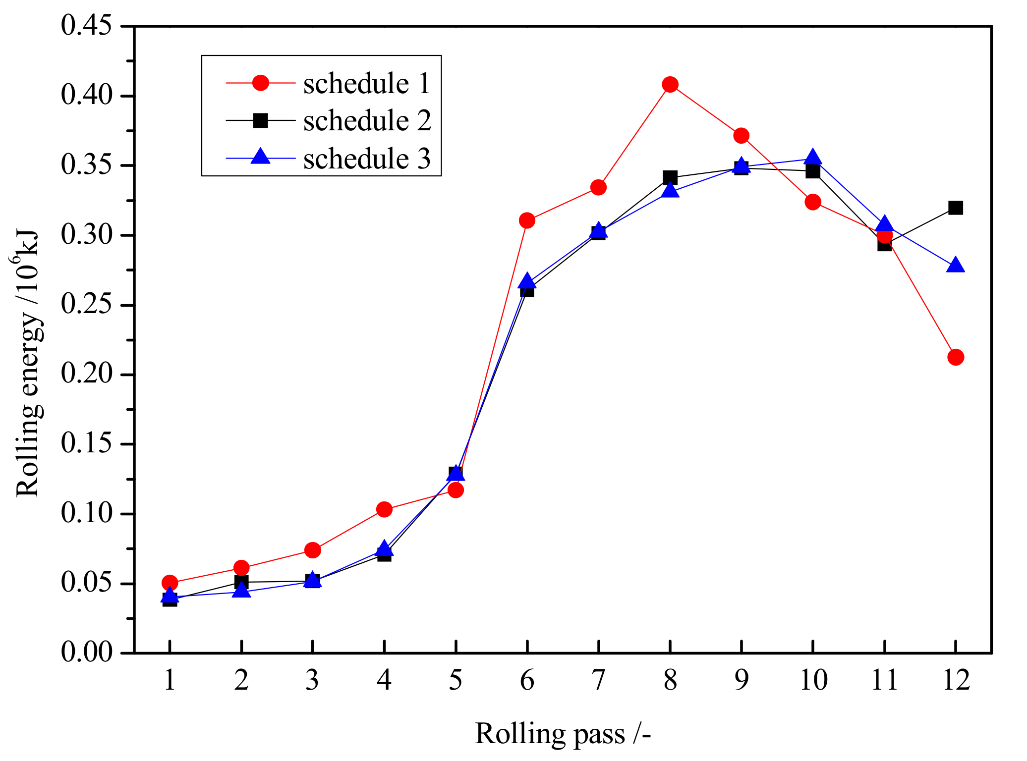
From the comparison between Schedule 1 and Schedule 2, it is shown that at the same tapping temperature (1180 °C), the heating energy is equal, and the total energy difference is derived from the rolling energy. It is effective to obtain a better schedule by solving the rolling energy function. Comparison between Schedule 2 and Schedule 3, when the tapping temperature changed from 1180 °C to 1181.9 °C, shows that the heating energy enhanced from 5.7368 × 10⁶ kJ to 5.7556 × 10⁶ kJ, but the rolling energy reduced from 2.5523 × 10⁶ kJ to 2.5269 × 10⁶ kJ, and the total energy was reduced about 1.5%. Figure 9 shows the rolling energy of each pass under the three schedules, and these schedules were satisfying the constraint conditions. The final Schedule 3 was effective for this 1580 mm line.
The convergent iteration curve is shown in Figure 10, the calculated time is less than 1.39 s, which can meet the timeliness of online applications.
Based on the above analysis and discussion, the proposed method can realize the rapid solution of the multi-objective function, and can also meet the requirements of equipment and process conditions. Meanwhile, the differential evolution algorithm is feasible to solve the multi-objective optimization problem, and the solving speed can meet the online application requirements. The purpose of reducing energy consumption in the whole production process was achieved, which can have a good guiding role in actual production.
5. Conclusions
Focusing on the whole process, the optimized schedule was obtained by minimizing the multi-objective function, in which the heating energy and rolling energy were both taken into consideration. In the solution of the multi-objective function, the differential evolution algorithm was used to find the optimal solutions. Finally, the tapping temperature and the thickness of each pass were both obtained, and the desired schedule can meet the constraint conditions. Meanwhile, the validity of the proposed method was verified by comparing it with the actual schedule and the single objective function, so the total energy was reduced by about 1.5% for a typical specification, and the purpose of reducing production energy consumption was achieved.
Author Contributions
Conceptualization, D.Z.; Formal analysis, J.S.; Methodology, X.C. and J.D.; Software, J.M.; Writing-original, Y.J. and W.P.; Writing-Review & Editing, W.P. All authors have read and agreed to the published version of the manuscript.
Funding
This research was funded by National Natural Science Foundation of China (51704067, 51634002), National Key R&D Program of China (2017YFB0304100), Natural Science Foundation of Shanxi Province, China (201901D111243) and Fundamental Research Funds for the Central Universities (N180704006, N180704005, N2004010).
Conflicts of Interest
The authors declare no conflict of interest.
| Symbol List | ||||
| Abbreviations | Instructions | Unit | Value | Position |
| Heating energy consumption | kJ | - | Equation (1) | |
| Drive motors energy consumption | kJ | - | Equation (1) | |
| Total pass number | - | - | Equation (1) | |
| Pass number of rough rolling | - | - | Equation (1) | |
| Pass number of finishing rolling | - | - | Equation (1) | |
| Mass of the slab | kg | - | Equation (2) | |
| Specific heat capacity of the slab | J/(kg·K) | - | Equation (2) | |
| Charging temperature of the slab | K | - | Equation (2) | |
| Tapping temperature of the slab | K | - | Equation (2) | |
| Energy conversion efficiency coefficient | - | - | Equation (2) | |
| Rolling power of the drive motor | kW | - | Equation (3) | |
| Rolling time during the strip through the roll | s | - | Equation (3) | |
| Rolling torque of the drive motor | N·M | - | Equation (4) | |
| Rotational speed of the drive motor | rad/min | - | Equation (4) | |
| Rolling force | kN | - | Equation (5) | |
| Arm coefficient | mm | - | Equation (5) | |
| Contact arc length | mm | - | Equation (5) | |
| Additional torque of the drive motor | N·M | - | Equation (5) | |
| Width of the rolling strip | mm | - | Equation (6) | |
| Influence coefficient of tension | - | - | Equation (6) | |
| Deformation resistance of the rolling strip | MPa | - | Equation (6) | |
| Basic deformation resistance of the rolling strip | MPa | - | Equation (7) | |
| Deformation temperature of the rolling strip | K | - | Equation (7) | |
| Deformation velocity of the rolling strip | s−1 | - | Equation (7) | |
| True strain of the rolling strip | - | - | Equation (7) | |
| Influence coefficient of stress state | - | - | Equation (8) | |
| Ambient temperature | K | 300 | Equation (9) | |
| Temperature change caused by ambient | K | - | Equation (9) | |
| Temperature change caused by water cooling | K | - | Equation (9) | |
| Temperature change caused by deformation | K | - | Equation (9) | |
| Temperature change caused by friction | K | - | Equation (9) | |
| Temperature change caused by conduction | K | - | Equation (9) | |
| Equivalent emissivity | - | 0.8 | Equation (10) | |
| Density of the strip | kg/m3 | 7850 | Equation (10) | |
| Heat transfer time | s | Equation (10) | ||
| Forced convection heat transfer coefficient | W/(m2·K) | - | Equation (11) | |
| Deformation efficiency coefficient | - | 0.50 | Equation (12) | |
| friction efficiency coefficient | - | 0.65 | Equation (13) | |
| speed difference between the work roll and strip | m/s | - | Equation (13) | |
| Contact heat flow coefficient of the work roll | - | 0.70 | Equation (14) | |
| Heat conduction coefficient of the strip | W/m·K | Equation (14) | ||
| Temperature of the work roll | K | - | Equation (14) | |
| Minimum reliable thickness | mm | - | Equation (17) | |
| Diameter of the work roll | mm | - | Equation (18) | |
| Maximum thickness ratio of pass i | % | - | Equation (19) | |
| Bite angle | - | - | Equation (20) | |
| Reduction | - | - | Equation (20) | |
| Friction angle | - | - | Equation (20) | |
| Friction coefficient | - | 0.3 | Equation (20) | |
| Maximum rolling force | kN | - | Equation (21) | |
| Maximum rolling power of drive motors | kW | - | Equation (22) | |
| Maximum torque of drive motors | N·M | - | Equation (23) | |
| Maximum rotational speed of drive motors | rad/min | - | Equation (24) | |
References
- Sun, J.; Peng, W.; Ding, J.G.; Li, X.; Zhang, D.H. Key Intelligent Technology of Steel Strip Production through Process. Metals 2018, 8, 597. [Google Scholar] [CrossRef] [Green Version]
- Boom, R. The discussions of best heating technology of rolling furnace. Ironamk. Steelmak. 2014, 41, 647–652. [Google Scholar] [CrossRef]
- Wang, Z.B.; Zhao, B.; Zhang, S.J. The discussions of best heating technology of rolling furnace. Beijing Energy Metall. Ind. 2008, 5, 8. [Google Scholar]
- Steinboeck, A.; Wild, D.; Kiefer, T. A fast simulation method for 1D heat conduction. Math. Comput. Simulat. 2011, 82, 392–403. [Google Scholar] [CrossRef]
- Kim, J.G.; Huh, K.Y.; Kim, I.T. Three-dimensional analysis of the walking beam type reheating furnace in hot strip mills. Numer. Heat Transf. 2000, 38, 589–609. [Google Scholar]
- Kim, M.A. Heat transfer model for the analysis of transient heating of the slab in a direct-fired walking beam type reheating furnace. Int. J. Heat Mass Transf. 2007, 50, 3740–3748. [Google Scholar] [CrossRef]
- Miao, C.; Kai, Y.; Liu, Y.F. Inverse estimation of transient heat flux to slab surface. J. Iron Steel Res. 2012, 19, 13–18. [Google Scholar]
- Suzuki, M.; Katsuki, K.; Imura, J.I. Simultaneous optimization of slab permutation scheduling and heat controlling for a reheating furnace. J. Process Control 2014, 24, 225–238. [Google Scholar] [CrossRef]
- Emadi, A.; Saboonchi, A.; Taheri, M. Heating characteristics of billet in a walking hearth type reheating furnace. Appl. Therm. Eng. 2014, 63, 396–405. [Google Scholar] [CrossRef]
- Morgado, T.; Coelho, P.J.; Talukdar, P. Assessment of uniform temperature assumption in zoning on the numerical simulation of a walking beam reheating furnace. Appl. Therm. Eng. 2015, 76, 496–508. [Google Scholar] [CrossRef]
- Han, S.H.; Baek, S.W.; Kim, M.Y. Transient radiative heating characteristics of slabs in a walking beam type reheating furnace. Int. J. Heat Mass Transf. 2009, 52, 1005–1011. [Google Scholar] [CrossRef]
- Casal, J.M.; Porteiro, J.; Miguez, J.L. New methodology for CFD three-dimensional simulation of a walking-beam type reheating furnace in steady state. Appl. Therm. Eng. 2015, 86, 69–80. [Google Scholar] [CrossRef]
- Depree, N.; Sneyd, J.; Taylor, S. Development and validation of models for annealing furnace control from heat transfer fundamentals. Comput. Chem. Eng. 2010, 34, 1849–1853. [Google Scholar] [CrossRef]
- Feliu, B.V.; Rivas, P.R.; Castillo, G.F.J. Simple fractional order controller combined with a Smith predictor for temperature control in a steel slab reheating furnace. Int. J. Control Autom. Syst. 2013, 11, 533–544. [Google Scholar] [CrossRef]
- Wang, W.; Li, H.X.; Zhang, J. A hybrid approach for supervisory control of furnace temperature. Control Eng. Pract. 2003, 11, 1325–1334. [Google Scholar] [CrossRef]
- Wang, Y.J.; Huang, J.W.; Su, C.; Li, H.G. Furnace thermal efficiency modeling using an improved convolution neural network based on parameter-adaptive mnemonic enhancement optimization. Appl. Therm. Eng. 2019, 149, 332–343. [Google Scholar] [CrossRef]
- Prieler, R.; Mayrhofer, M.; Gaber, C.; Gerhardter, H.; Schluckner, C.; Landfahrer, M.; Eichhorn-Gruber, M.; Schwabegger, G.; Hochenauer, C. CFD-based optimization of a transient heating process in a natural gas fired furnace using neural networks and genetic algorithms. Appl. Therm. Eng. 2018, 138, 217–234. [Google Scholar] [CrossRef]
- Jiang, X.; Hu, X.L.; Liu, X.H.; Wang, G.D. Application of compound equal load distribution method in rough rolling schedule. J. Iron Steel Res. 2006, 18, 26–29. [Google Scholar]
- Shen, X.G.; Han, N.; Shen, H.Y. Application of synergetic artificial intelligence to the scheduling in the finishing train of hot strip mills. J. Mater. Process. Technol. 1996, 60, 405–408. [Google Scholar]
- Li, H.J.; Wang, G.D.; Xu, J.Z. Optimization of draft schedules with variable metric hybrid genetic algorithm during hot strip rolling. J. Iron Steel Res. Int. 2007, 19, 33–36. [Google Scholar]
- Li, W.G.; Liu, C.; Bian, H.; Liu, X.H. Optimization calculation strategy of load distribution for hot strip mills. J. Iron Steel Res. 2017, 29, 391–396. [Google Scholar]
- Jia, S.J.; Li, W.G.; Liu, X.H.; Du, B. Multi-objective load distribution optimization for hot strip mills. J. Iron Steel Res. Int. 2013, 20, 27–32. [Google Scholar] [CrossRef]
- Li, H.J.; Xu, J.Z.; Wang, G.D. Improvement on conventional load distribution algorithm in hot tandem mills. J. Iron Steel Res. Int. 2007, 14, 36–41. [Google Scholar] [CrossRef]
- Li, W.G.; Liu, X.H.; Guo, Z.H. Multi-objective optimization for draft scheduling of hot strip mill. J. Cent. South Univ. 2012, 19, 3069–3078. [Google Scholar] [CrossRef]
- Qi, X.D.; Wang, T.; Xiao, H. Optimization of pass schedule in hot strip rolling. J. Iron Steel Res. Int. 2012, 19, 25–28. [Google Scholar] [CrossRef]
- Pan, Q.K.; Gao, L.; Wang, L. A multi-objective hot-rolling scheduling problem in the compact strip production. Appl. Math. Model. 2019, 73, 327–348. [Google Scholar] [CrossRef]
- Peng, W.; Liu, Z.Y.; Yang, X.L.; Zhang, D.H. Optimization of temperature and force adaptation algorithm in hot strip mill. J. Iron Steel Res. Int. 2014, 21, 300–305. [Google Scholar] [CrossRef]
- Liu, E.Y.; Peng, L.G.; Yuan, G. Advanced run-out table cooling technology based on ultra-fast cooling and laminar cooling in hot strip mill. J. Cent. South Univ. 2012, 19, 1341–1345. [Google Scholar] [CrossRef]
- Stone, M.D. Rolling of thin strip. Iron Steel Eng. 1953, 30, 61–65. [Google Scholar]
- Storn, R.; Price, K. Differential Evolution-A Simple and Efficient Adaptive Scheme for Global Optimization over Continuous Space, TR-95-012; International Computer Science Institute: Berkeley, CA, USA, 1995. [Google Scholar]
- Price, K.; Storn, R.; Lampinen, J. Differential Evolution-A Practical Approach to Global Optimization; Springer: Berlin/Heidelberg, Germany, 2005. [Google Scholar]
- Peng, W.; Zhang, D.H.; Zhao, D.W. Application of parabolic velocity field for the deformation analysis in hot tandem rolling. Int. J. Adv. Manuf. Technol. 2017, 91, 2233–2243. [Google Scholar] [CrossRef]
- Qi, K.M.; Ding, H. Material Forming Technology; Metallurgical industry press: Beijing, China, 2013. [Google Scholar]
- Ginzburg, V.B.; Ballas, R. Fundamentals of Flat Rolling Manufacturing Engineering and Materials Processing; CRC Press: Boca Raton, FL, USA, 2000. [Google Scholar]
Figure 1.
Layout of the typical traditional hot rolling line.

Figure 2.
Flow chart of total energy calculation.

Figure 3.
Heat flows during the strip transportation.

Figure 4.
Flow chart of multi-objective function solution.

Figure 5.
The influence of initial and tapping temperature on heating energy.

Figure 6.
The influence of tapping temperature on heating energy and rolling energy.

Figure 7.
Comparison of total energy between the actual schedule and optimized schedule (1170–1210 °C).
Figure 7.
Comparison of total energy between the actual schedule and optimized schedule (1170–1210 °C).

Figure 8.
Comparison of heating energy, rolling energy and total energy of three schedules.

Figure 9.
Comparison of rolling energy of each pass (tapping temperature 1180 °C).

Figure 10.
Convergence iterative curve for solving the multi-objective function.


Table 1.
Main plant parameters of hot tandem production line.
| Parameter | R | F1 | F2 | F3 | F4 | F5 | F6 | F7 |
|---|---|---|---|---|---|---|---|---|
| Roll Diameter/mm | 1100 | 800 | 800 | 800 | 800 | 700 | 700 | 700 |
| Max Rolling Force/kN | 40,000 | 40,000 | 40,000 | 40,000 | 40,000 | 34,000 | 34,000 | 34,000 |
| Max Torque/(kN·m) | 4300 | 2000 | 2000 | 2000 | 1500 | 1500 | 1200 | 1200 |
| Max Motor Power/kW | 7500×2 | 8000 | 8000 | 8000 | 8000 | 8000 | 7500 | 7500 |
| Max Motor Speed (rad s/−1) | 700 | 450 | 450 | 450 | 450 | 450 | 600 | 600 |
Table 2.
Regression coefficient in deformation resistance model.
| Coefficient | a1 | a2 | a3 | a4 | a5 | a6 | a7 |
|---|---|---|---|---|---|---|---|
| Value | 5.0 | −0.0588 | 0.12828 | −0.041 | 1.3 | 0.41 | 2.80 |
Table 3.
Main process requirements constraints of Q235 steel.
| Parameter | R | F1 | F2 | F3 | F4 | F5 | F6 | F7 |
|---|---|---|---|---|---|---|---|---|
| Thickness Ratio Range *1/% | 60% | 40–50% | 35–45% | 30–40% | 25–35% | 25–35% | 20–30% | 10–20% |
| Max Bite Angle *2/° | 18.30 | 18.47 | 18.74 | 19.25 | 20.59 | 17.30 | 17.72 | 18.16 |
| Min Thickness *3/mm | 55.62 | 56.68 | 58.29 | 61.47 | 70.25 | 36.18 | 37.94 | 39.83 |
Table 4.
Rolling schedule of Q235 steel used in actual production process (2.0mm).
| Pass | R1 | R2 | R3 | R4 | R5 | F1 | F2 | F3 | F4 | F5 | F6 | F7 |
|---|---|---|---|---|---|---|---|---|---|---|---|---|
| Thickness/mm | 145.0 | 103.0 | 72.0 | 48.0 | 33.0 | 16.65 | 9.44 | 5.69 | 3.90 | 2.92 | 2.33 | 2.00 |
| Thickness ratio/% | 27.50 | 28.97 | 30.10 | 33.33 | 31.25 | 49.55 | 43.30 | 39.72 | 31.46 | 25.13 | 20.21 | 14.16 |
| Velocity m/s | 2.5 | 3.0 | 3.5 | 3.6 | 4.0 | 1.20 | 2.12 | 3.51 | 5.13 | 6.85 | 8.58 | 10.00 |
Table 5.
Details of three schedules.
| Parameter | schedule | R1 | R2 | R3 | R4 | R5 | F1 | F2 | F3 | F4 | F5 | F6 | F7 |
|---|---|---|---|---|---|---|---|---|---|---|---|---|---|
| Thickness/mm | 1 | 145.0 | 103.0 | 72.0 | 48.0 | 33.0 | 16.65 | 9.44 | 5.69 | 3.90 | 2.92 | 2.33 | 2.00 |
| 2 | 153.0 | 112.7 | 84.41 | 60.48 | 39.19 | 19.91 | 11.04 | 6.66 | 4.43 | 3.16 | 2.47 | 2.00 | |
| 3 | 151.5 | 114.7 | 85.8 | 60.7 | 39.3 | 19.8 | 10.9 | 6.64 | 4.40 | 3.13 | 2.43 | 2.00 | |
| Velocity/m/s | 1 | 2.50 | 3.00 | 3.50 | 3.60 | 4.00 | 1.20 | 2.12 | 3.51 | 5.13 | 6.85 | 8.58 | 10.00 |
| 2 | 2.50 | 3.00 | 3.50 | 3.60 | 4.00 | 1.00 | 1.81 | 3.00 | 4.52 | 6.32 | 8.09 | 10.00 | |
| 3 | 2.50 | 3.00 | 3.50 | 3.60 | 4.00 | 1.01 | 1.83 | 3.01 | 4.54 | 6.39 | 8.23 | 10.00 | |
| Force/kN | 1 | 21,608 | 21,718 | 21,716 | 23,462 | 23,249 | 26,950 | 24,071 | 23,724 | 19,960 | 15,296 | 13,491 | 9970 |
| 2 | 18,578 | 20,042 | 18,426 | 20,138 | 26,002 | 25,072 | 23,243 | 21,825 | 19,674 | 16,306 | 13,432 | 13,343 | |
| 3 | 19,077 | 18,363 | 18,471 | 20,774 | 25,874 | 25,263 | 23,196 | 21,370 | 19,680 | 16,531 | 13,781 | 12,022 | |
| Temperature/°C | 1 | 1142.8 | 1133.8 | 1121.0 | 1099.1 | 1050.3 | 1015.1 | 993.4 | 971.1 | 947.6 | 924.6 | 901.8 | 880.1 |
| 2 | 1143.2 | 1135.1 | 1124.6 | 1108.6 | 1073.4 | 1037.8 | 1016.2 | 993.2 | 969.7 | 946.2 | 922.9 | 899.7 | |
| 3 | 1145.0 | 1136.9 | 1126.6 | 1110.9 | 1075.6 | 1040.0 | 1018.3 | 995.4 | 971.6 | 948.0 | 924.5 | 901.4 | |
| Power/kW | 1 | 13,122 | 13,551 | 13,331 | 12,739 | 11,044 | 4440 | 4777 | 5831 | 5306 | 4628 | 4290 | 3036 |
| 2 | 10,541 | 12,329 | 10,948 | 11,031 | 14,450 | 3729 | 4307 | 4873 | 4972 | 4942 | 4195 | 4565 | |
| 3 | 10,954 | 10,825 | 11,057 | 11,599 | 14,369 | 3798 | 4322 | 4730 | 4989 | 5070 | 4389 | 3965 | |
| Energy/×106 kJ | 1 | 0.051 | 0.061 | 0.074 | 0.103 | 0.117 | 0.311 | 0.334 | 0.408 | 0.371 | 0.324 | 0.300 | 0.213 |
| 2 | 0.039 | 0.051 | 0.052 | 0.071 | 0.129 | 0.261 | 0.302 | 0.341 | 0.348 | 0.346 | 0.294 | 0.320 | |
| 3 | 0.041 | 0.044 | 0.052 | 0.074 | 0.128 | 0.266 | 0.303 | 0.331 | 0.349 | 0.355 | 0.307 | 0.278 |
© 2020 by the authors. Licensee MDPI, Basel, Switzerland. This article is an open access article distributed under the terms and conditions of the Creative Commons Attribution (CC BY) license (http://creativecommons.org/licenses/by/4.0/).
Share and Cite
MDPI and ACS Style
Peng, W.; Ma, J.; Chen, X.; Ji, Y.; Sun, J.; Ding, J.; Zhang, D. Optimization of the Schedule for the Whole Process in Hot Strip Manufacturing. Metals 2020, 10, 717. https://doi.org/10.3390/met10060717
AMA Style
Peng W, Ma J, Chen X, Ji Y, Sun J, Ding J, Zhang D. Optimization of the Schedule for the Whole Process in Hot Strip Manufacturing. Metals. 2020; 10(6):717. https://doi.org/10.3390/met10060717
Chicago/Turabian StylePeng, Wen, Jianyang Ma, Xiaorui Chen, Yafeng Ji, Jie Sun, Jinggou Ding, and Dianhua Zhang. 2020. "Optimization of the Schedule for the Whole Process in Hot Strip Manufacturing" Metals 10, no. 6: 717. https://doi.org/10.3390/met10060717
Note that from the first issue of 2016, this journal uses article numbers instead of page numbers. See further details here.