Unsharpness of Thermograms in Thermography Diagnostics of Electronic Elements
by
 , ,
, ,
Krzysztof Dziarski
1,*, 
Arkadiusz Hulewicz
2,
Grzegorz Dombek
1,
Ryszard Frąckowiak
1 and
Grzegorz Wiczyński
2 1
Institute of Electric Power Engineering, Poznan University of Technology, Piotrowo 3A, 60-965 Poznan, Poland
2
Institute of Electrical Engineering and Industry Electronics, Poznan University of Technology, Piotrowo 3A, 60-965 Poznan, Poland
*
Author to whom correspondence should be addressed.
Electronics 2020, 9(6), 897; https://doi.org/10.3390/electronics9060897
Submission received: 30 April 2020
/
Revised: 20 May 2020
/
Accepted: 26 May 2020
/
Published: 28 May 2020
(This article belongs to the Section Circuit and Signal Processing)
Abstract
:Work temperature is a factor, which has a strong influence on the work of a semiconductor electronic element. Operation of an electronic element in an excessive temperature causes the element not to work correctly. For this reason, monitoring the temperature of the element is necessary. One of the methods, which allows the monitoring of electronic element temperature is thermography. This non-contact method can also be used during the operation of the electronic element. The reading of a thermal camera depends on several factors. One of these factors is the sharpness of the registered thermograms. For this reason, research was carried out to develop a simple tool that allows a clear classification of thermograms of electronic elements into sharp and unsharp thermograms. In the research carried-out, the sharpness of the registered thermograms of electronic elements was determined by different sharpness measures. In the research, it was shown that in the case of thermograms classified as sharp, a smaller error of temperature measurement was obtained with the use of a thermal imaging camera.
1. Introduction
Performing in-service tests of all types of devices increases the safety of their operation and their reliability [1,2]. Early detection of improper operation of semiconductor electronic components prevents damage to the entire device and extends the time of failure-free operation. Damage to electronic components is most often manifested in a change in their temperature, which is an increase in most cases. Therefore, thermovision observations are an effective diagnostic method. This non-contact method [3] allows recording temperature distribution on housings of semiconductor components and radiators [4]. For example, it is possible to detect a local temperature increase on the housing of an element, the so-called hot spot.
Thermovision diagnostics makes it possible to record changes in temperature values in real time. Consequently, early detection of potential damage is possible [5]. The result of thermovision temperature measurement depends on several factors. The basic factor is the value of the emissivity coefficient of the observed object (surface). This coefficient is the quotient of the intensity of radiation emitted by the observed surface and radiation emitted by a black body at the same temperature [6]. Other factors include, among others, the distance between the thermographic camera and the object, object observation angle, reflection of radiation emitted by unobserved objects, thermogram sharpness. The last factor is seldom included in the assessment of measurement reliability. A lack of sharpness of a thermogram can be caused by two main reasons. The first one is incorrect selection of the angular position of the lens focusing ring. The second reason is insufficient depth of image of thermographic cameras. The impact of the latter reason is mostly visible in cases of unfavorable geometry of thermogram scenes (surfaces of the observed object stay at a different distance from the lens).
Thermogram sharpness assessment, which is a graphic representation of temperature distribution [7] on a selected surface, is a complex task. The result of sharpness assessment depends on, among other factors, personal predispositions of the observers. The subjective perception of sharpness makes it impossible to obtain a thermogram which is sharp for each observer. Along with the change in thermogram sharpness, the reading of a thermographic camera changes. Therefore, the difference between the thermovision result of the temperature measurement and the actual temperature of the observed surface increases [8,9].
When collecting thermograms for scientific and technical research, the subjective visual impression of an observer should be replaced by an objective assessment of thermogram quality by means of a measure of sharpness expressed in a specific mathematical formula. Many measures of image sharpness have been proposed in the literature. The proposed measures can be divided into two categories: measures using the variability of image content in the spatial domain, and measures studying the image as a result of the transformation carried out.
Measures using the variability of image content include a measure based on the blur of image parts [10,11]. One of these measures of sharpness based on edge width is called JNB (just noticeable blur) [12]. There is another sharpness measure based on blur detection probability called CPBD (cumulative probability of blur detection) [13] and a statistical method of determining image sharpness [14,15]. This group of measures also includes the sharpness measure called S3 (spectral and spatial sharpness) [16], a measure using the natural scene statistics of local luminance coefficients (blind referenceless image spatial quality evaluator) [17] and the measures presented in [18,19,20,21,22].
Measures examining image sharpness as a result of transformation include, inter alia, the LPC (local phase coherence) measure, based on local phase coherence [23]. There are also other methods using the distribution of transformation coefficients. Their examples include the distortion identification-based image verity and integrity evaluation (DIIVINE) [24] and measures described in [25,26,27]. The measures of sharpness described in [10,11,12,13,14,15,16,17,18,19,20,21,22,23,24,25,26,27] have been used to determine sharpness in photography.
The issue of selecting the sharpness of an image does not concern photography alone. As previously mentioned, the result of temperature measurement using a thermographic camera depends on thermogram sharpness (or rather a lack of sharpness). It can be presumed that the measures of image sharpness proposed in [10,11,12,13,14,15,16,17,18,19,20,21,22,23,24,25,26,27] can also be used to assess thermograms. Attempts can be found in the literature to determine thermogram sharpness with the use of some of these measures, e.g., [28,29]. When adapting sharpness measures from photography, one should bear in mind the differences between thermal imaging and video cameras. For example, thermal imaging cameras compared to video cameras are characterized by lower matrix resolution, lower depth of field, and greater defocusing (caused by a wider range of spectral sensitivity). Under field conditions, and also often in the laboratory, it is difficult to assess the sharpness of the recorded thermogram unambiguously. The issue of assessing thermogram sharpness is particularly evident when using a macro lens to watch small objects. The use of mathematical measures of image sharpness generates certain values. On this basis, images should be classified into sharp and out of focus. Neural networks are an effective tool supporting this division [30]. Additionally, in the case of thermograms, it is possible to classify them into sharp and unsharp using neural networks [31,32]. It is interesting to note the report on the use of a neural network in thermogram analysis when searching for defects [33].
This work presents the results of thermovision diagnostics of an electronic element. Presented are examples of thermograms illustrating the effect of the lack of their sharpness on the result of temperature measurement of the observed element. A list of image sharpness measures (selected on the basis of a literature review) is presented. The results of research on the effect of angular position α of the focusing adjustment ring and the distance d between the observed element and the lens of thermographic camera on the values of thermogram sharpness measures have been presented. The results of this research indicate that classification of thermograms in terms of sharpness requires the use of appropriate tools. From a practical point of view, one should seek to use the simplest tools that allow achieving the desired effect. Therefore, this work proposes the use of a perceptron for the classification of thermograms. To obtain the dataset to teach the perceptron, surveys were conducted with the participation of over 100 volunteers. It has been shown that using the proposed thermogram quality assessment tool can increase the reliability of thermovision diagnostics.
2. Result of Temperature Measurement by Thermovision versus Thermogram Unsharpness
A recorded thermogram is sharp when the IR rays that reach the camera refract in the objective lens in such a way that they intersect in the matrix of IR detectors. In this case, the object’s image emerges on the detector matrix. Otherwise, the thermogram is out of focus, and the energy absorbed by detectors does not allow obtaining the correct matrix response (i.e., the result of temperature measurement). This is one of the uncertainty factors of temperature measurement by thermal imaging camera. The refraction angle of IR radiation in the lens (and thus the point of intersection of IR rays entering the lens) depends on lens position relative to the IR detector array and the object observed. In the case of thermal imaging cameras, lens position can be adjusted using the focusing adjustment ring placed on the lens. The place where the image emerges depends on the position of the lens relative to the surface observed. For this reason, the sharpness of the recorded thermogram depends on the distance between the lens and the surface observed.
A change in the reading of thermal imaging camera accompanying focus changes was detected by the authors of this publication during temperature measurements of various objects. For example, it was noticed during observation of a 2.3 mm × 2.1 mm Pt1000 resistance temperature sensor [34]. Thermograms that illustrate the effect of a lack of sharpness on the reading of the Flir E50 thermal imaging camera, including the result of measuring the temperature ϑm of an element with a constant temperature value ϑp = 103.5 °C, are shown in Figure 1. Temperature ϑc was measured by an electric method (the temperature value was determined on the basis of the value of resistance measurement of the Pt1000 sensor). The correct thermovision measurement of the temperature of sensor surface requires the knowledge of the emissivity coefficient ε of that surface. The value of ε of the observed surface was determined by equalizing the measurement result ϑm of thermal imaging camera and the result of the electrical measurement of temperature ϑp.
Figure 1 shows that the result of temperature measurement ϑm with the use of a thermal imaging camera depends on thermogram sharpness. The presented phenomenon occurred irrespective of taking into account the climatic conditions prevailing during the measurement (by making appropriate settings of the thermal imaging camera, i.e., ε = 0.7, reflected temperature of 24 °C, object–lens distance of 33 mm, air temperature of 24 °C, relative humidity of 40%, exposure time longer than 3 s).
3. Assessment of Impact of Thermogram Unsharpness on the Error of Temperature Measurement by a Thermal Imaging Camera
Since the result of thermovision temperature measurement depends on thermogram unsharpness, the question which should be asked is to what extent the thermogram could be out of focus, so that the error of temperature measurement Δϑ was acceptably small. To answer this question, the effect of unsharpness on the measurement result was assessed by linking the value of sharpness measure with measurement error values. Temperature measurement error Δϑ was defined as the difference of thermovision measurement result ϑm and the correct valueϑp [35]:
Δϑ = ϑm − ϑp.
In order to link thermogram quality with the error in temperature measurement, it is necessary to determine thermogram sharpness using an appropriate measure. In order to select the most effective measure, comparative studies of the results of mathematical sharpness measures and the subjective visual impressions of volunteer observers were conducted. Six series (sets) of thermograms were used for comparisons. These sets were also used to teach the perceptron (Section 6). Thermovision measurements of the electronic element were made using a Flir E50 camera (Flir, Wilsonville, OR, USA) [36] fitted with an additional macro Close-up lens 2× T197214. The camera spatial resolution was 240 × 180 pixels. In the event of using an additional lens, it was possible to obtain, for this camera spatial resolution, a field of view of a single detector with an edge length of 67 µm. The achieved spatial resolution was sufficient to place at least nine fields of a single detector on the observed surface, even for the largest lens—observed element distance d of 43 mm.
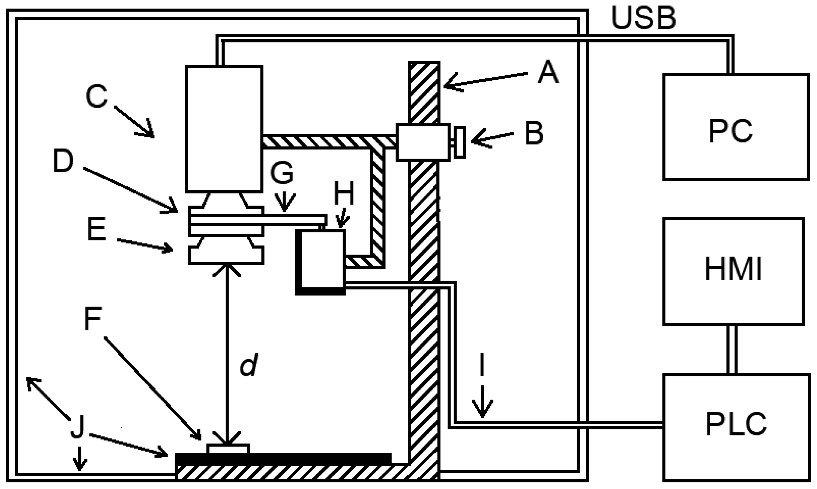
The camera was mounted on a tripod, which made it possible to change the lens position in relation to the observed surface with a resolution equal to 1 mm. In addition, a stepper motor making it possible to change the angular position α with a step of Δa = 1.5° was mounted on the tripod. The tripod was placed inside a chamber. In order to eliminate reflections that might interfere with thermovision measurements, the chamber walls and shiny surfaces (e.g., motor housing) were lined with black polyurethane foam. Positioning the tripod inside the chamber enabled the measurement conditions to be stabilized. The control system comprising a PLC (programmable logic controller) and a touch panel was placed outside of the chamber. The measuring system diagram is shown in Figure 2.
Thermographic camera settings were not changed whilst performing the thermograms. They were selected specifically for the conditions inside the chamber. Whilst the first three series were run, the distance d was constant. Only the sharpness of the recorded thermogram was altered by changing the angle α with a step of Δa = 1.5°. Whilst performing the remaining three series of thermograms, the α value was constant. It was selected so as to obtain a sharp thermogram for distance d of 33 mm (working distance suggested by the macro lens manufacturer). The distance d was changed from d = 23 mm to d = 43 mm.
4. Mathematical Sharpness Measures Used to Assess the Quality of Thermograms
For each of the recorded thermograms, sharpness was determined with the use of the following sharpness measures (Equations (2)–(11)).
Variance D2 is the simplest measure of image sharpness. For the thermogram with the dimensions of N × M, the variance is calculated as follows [19]:
where:
An expression that makes it possible to represent image sharpness by means of EOG (energy of gradient) can be presented using equation [19]:
Another measure to describe image sharpness is EOL (energy of Laplacian). In order to determine image sharpness using this measure, use the following equation [19]:
Another sharpness measure is SML (sum modified Laplacian) and it has been proposed in the literature [26]. Nayar noticed that in the case of the Laplace operator, second derivatives in the x and y directions may have opposite signs and cancel each other reciprocally. He proposed a modified Laplacian (ML) of discrete expression. ML (modified Laplacian) was presented as:
The step was designated as “h“. In the works performed by the authors, step “h” was always 1 [28]:
where N defines the size of a window used to determine image sharpness.
The penultimate sharpness measure used in this work is SF (spatial frequency). Spatial frequency is not a new measure of sharpness, but a modified version of the measure consisting in measuring the energy of gradient of an image (EOG). Spatial frequency SF can be defined as follows [19,29]:
where RF (row frequency) is the frequency of the row [26]:
while CF (column frequency) is, respectively, the frequency of the column [19]:
The last measure considered in this work is Tenengrad. It is a measure based on determining the magnitude of gradient using the Sobel operator. In order to use this measure of sharpness, one should use the following relationship [19]:
The obtained values of sharpness measures were normalized according to the following equation:
where V’ is the normalized value of sharpness measure for a given thermogram, V is the sharpness measure value for a given thermogram obtained from the performed calculations (pre-normalization), Vmin is the minimum sharpness value obtained as a result of calculations for an entire series, Vmax is the maximum sharpness value obtained as a result of calculations for an entire series.
5. Comparing the Mathematical Values of Thermogram Sharpness with the Observers’ Visual Impressions
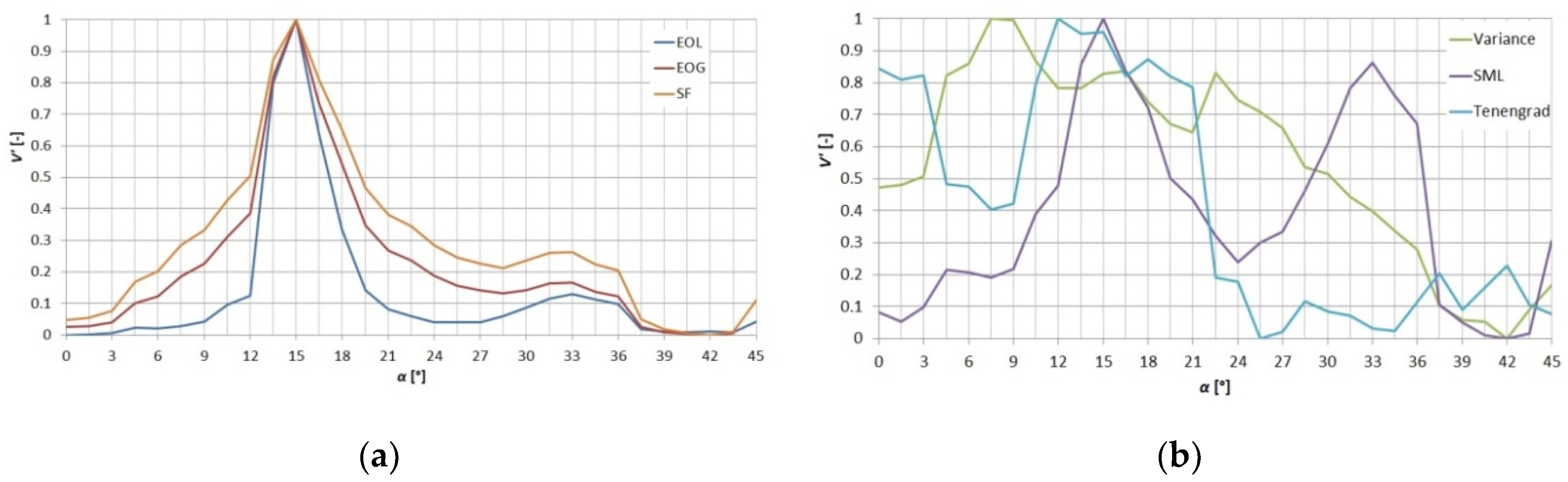
When measuring the sharpness of a thermogram, a matrix was uploaded representing the color saturation assigned to the estimated temperature of each sensor. The dimensions of the uploaded matrix depend on the resolution of the IR radiation sensor array in the camera used. Thermograms made with the use of the Flir MSX® (multi-spectral dynamic imaging) function are an exception. In such a case, the size of the matrix will depend on MSX resolution of the camera. In the scope of the works, thermograms in shades of grey were made. Once a thermogram was uploaded, an M × N matrix was obtained corresponding to the sensor array resolution. For a matrix with elements in an 8-bit representation, the numbers fall in the range of 0–255, where 0 is assigned to black and 255 is assigned to white [37]. The remaining numbers in the set are assigned to various shades of grey. For each thermogram, the sharpness measure values ofthe Equations (2)–(11) were determined. At the beginning, thermogram sharpness was determined in those series where the change in blur was obtained by changing the angular position α (series 1–3). The determined values of sharpness measures are presented on the characteristics V’ = f(α, d = const) (Figure 3), where V’ was computed according to Equation (12). Due to the similar shape of the relationship V’ = f(α) for the series of measurements 1–3, Figure 3 shows the results obtained for series 3. In order to improve the transparency of the presented characteristics, calculation results for the measures of EOL, SF, EOG, and variance, SML, Tenengrad are presented separately.
When analyzing the relationships shown in Figure 3a, it can be seen that the extremes overlap for all the characteristics obtained. The mutual coverage of the extremes results from the similarity of the applied measures, which are based on edge blurring in two directions (vertical and horizontal). As the value of α increases, sharpness increases until it reaches its maximum. After reaching the maximum along with the increase of value α, a smooth decrease in the sharpness of the thermogram was observed. The extremes of the characteristics shown in Figure 3b do not coincide.
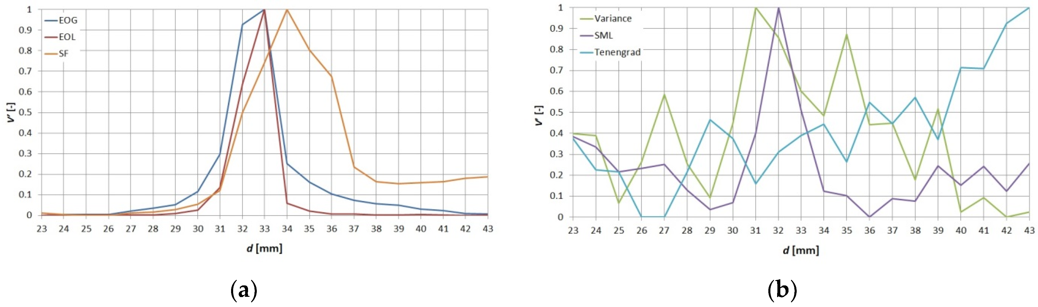
Figure 3 shows the dependence of the sharpness values on the angular position. To determine the effect of distance d on the blurring of thermograms, the values of sharpness measures for thermograms in the series of measurements 45 were calculated. The results of the calculations are presented on the characteristics V’ = f(d,α = const) (Figure 4). For better transparency, the calculations results for EOL, SF, and EOG, and for variance, SML and Tenengrad, are presented separately. Due to the similar shape of the relationship V’ = f(α) for the series of measurements 4–6, Figure 3 shows the results obtained for series 5.
In Figure 4, a consistent location of the extremes of the dependence V’ = f(d) was obtained for EOL and EOG measures. There was a slight shift for SF and SML measures. However, different characteristics were obtained for variance and Tenengrad.
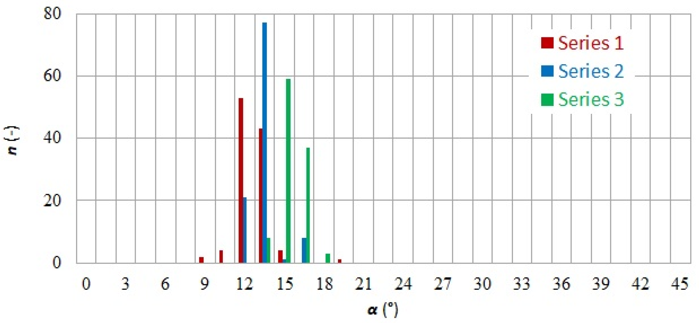
The set of thermograms subjected to analysis using mathematical measures of sharpness was shown to a group of observers. As the individual thermograms were presented, the observers were requested to give opinions about their sharpness. The task was to indicate the thermogram with the best sharpness within a given series. The observers’ answers are presented in diagrams in Figure 5 and Figure 6. The number of observers who pointed at a given thermogram as sharp is marked with the symbol n.
Comparing the waveforms of V’ = f(α) and V’ = f(d) presented in Figure 3 and Figure 4 with the observers’ responses presented in Figure 5 and Figure 6, it can be noticed that not all sharpness measures could be used. Sharpness measures based on edge blur (EOG, EOL) and a measure using the modified Laplacian SML (sum modified Laplacian) proved to be the best. The normalized courses of sharpness values of the angle α and distance d functions of these measures were closest to the observers’ visual impressions. Figure 7 shows the final selection of the comparison of the geometric mean value of the available correlation r between the relationship V′= f(α) and the observers’ indications and the value of r between the relationship V′ = f(d) and the observers’ indications.
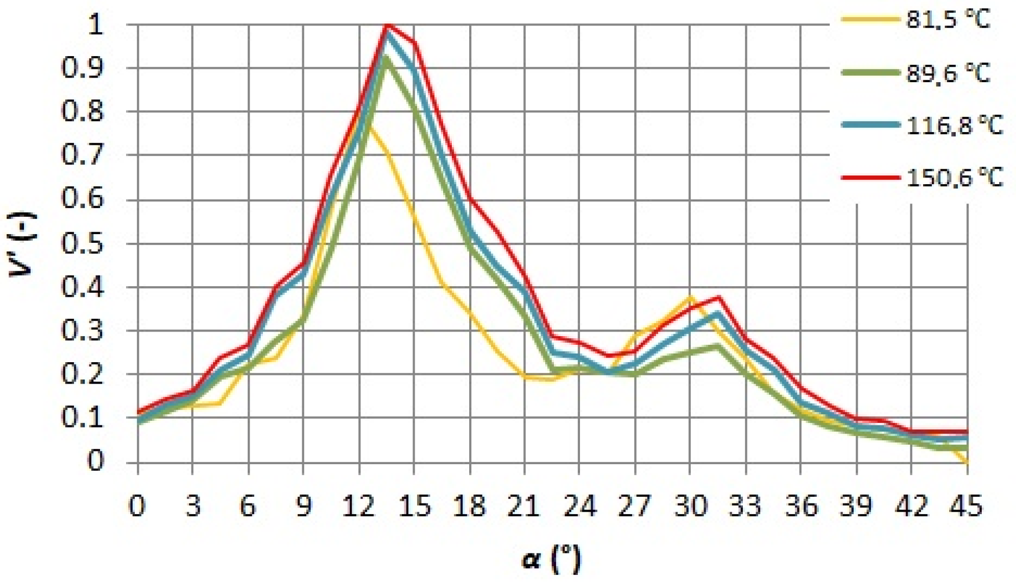
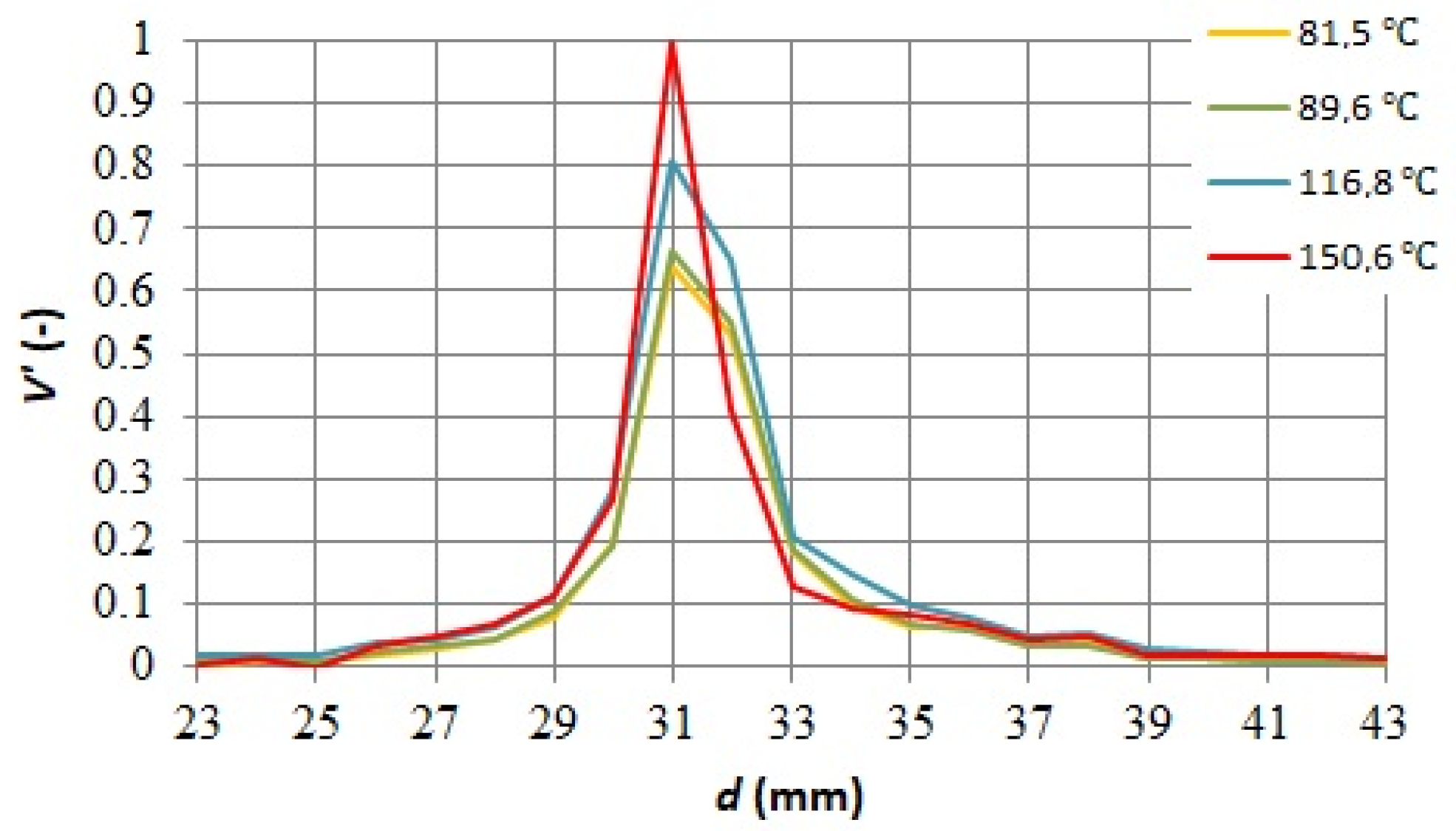
Based on the analysis and bearing in mind the geometric mean values r and ease of implementation, EOG was selected from among the applied measures for further work. Application of this measure required the least amount of calculations. The relationships V’ = f(α) and V’ = f(d) for different temperature values ϑp are presented in Figure 8 and Figure 9.
6. Automatic Classification of Thermograms with the Use of a Perceptron
When analyzing the relationships shown in Figure 3, Figure 4, Figure 5 and Figure 6, it can be noticed that the shape of waveform V’ = f(α) and V’ = f(d) depends on the sharpness measure used. It can also be stated that telling apart sharp and not sharp thermograms is not simple and unambiguous. For this reason, it was decided to apply automatic classification of thermograms.
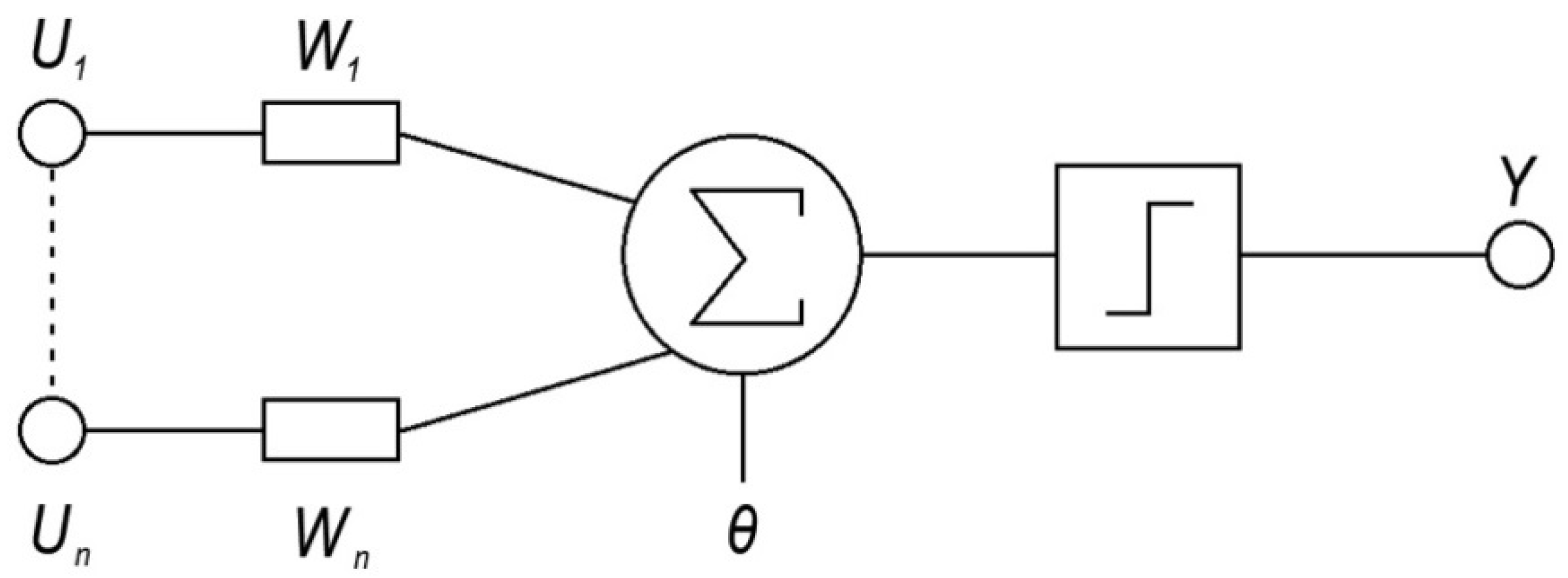
In order to automatically classify thermograms into sharp and not sharp, the authors decided to use a neural network consisting of one element: a single perceptron. A perceptron is an individual element of a neural network using Heaviside’s unit step function. It is the simplest solution making it possible to split data into two subgroups. When choosing a perceptron, it was decided to check whether such a simple element would achieve the desired effect, i.e., an effective classification of thermograms into sharp and not sharp. The implementation of a single perceptron does not require extensive knowledge and it is simpler than using more advanced solutions. A single perceptron is composed of any number of inputs U, input weights W, summing element, summing block, bias θ, Heaviside function value computation block, and the output. The perceptron design is shown in Figure 10.
Value Y generated as perceptron output may be described using the relationship expressed in the following equation:
A perceptron with one input was used for the purpose of these works. Normalized sharpness obtained by EOG was used as the perceptron input value U. The reasoning for selecting this measure is given in Section 3. In order to acquire the desired output value Y, an appropriate input weight W and bias θ need to be selected. The bias value and perceptron input weights can be chosen arbitrarily [38]. One of the methods for selecting bias and weight values is training the neural network using a training dataset comprising a training vector and an assumed response vector. The simple perceptron learning algorithm (SPLA) [39] makes it possible to train neural networks using a training values dataset. A similar, modified method was decided to be used in these works. For that purpose, a training vector and an assumed response vector had to be obtained. A series of tests was conducted. One hundred and seven people from both sexes, aged between 21 and 24, participated in the research. They took part in the study on a voluntary basis and were not in any relationship with the researchers. During the test, the observers were to select the sharpest and the least sharp thermogram in a set of thermograms. All tests were conducted using the same equipment and under the same conditions. The test yielded six training vectors (one for each series of thermograms) and six response vectors (one for each series of thermograms performed in 3) and six response vectors (one for each series of thermograms performed in 3). Each of the obtained training vectors comprised 214 elements, out of which 107 elements were normalized EOG (energy of gradient) thermogram values considered to be sharp. The remaining 107 vector elements were normalized EOG thermogram values considered as not sharp. The response vector comprised zeros and ones depending on whether it corresponded to a training vector value containing an EOG value corresponding to a sharp (logical 1) or not sharp (logical 0) thermogram. Once the training dataset was obtained, perceptron training began.
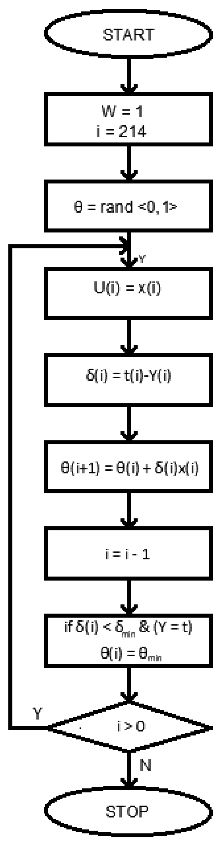
For the perceptron in question, with a single input, 1 may be chosen as the weight. There is no need to categorize inputs. Due to the fact that Heaviside’s unit step function was used, it was impossible to achieve the goal of thermogram classification. It was decided that the bias value would be variable, which was in fact a shift of the activation function along the OX axis. The initial bias value was a random value between 0 and 1. Then, the first value from the training vector was fed as the perceptron input. The generated output value Y was subtracted from the assumed perceptron response. That is how update correction δ was computed. Then, the value of correction δ was multiplied by the perceptron input value for that particular iteration x. Finally, a new value of bias θ was computed as the value of θ from the previous iteration plus correction δ. Two hundred and fourteen iterations were performed for all 214 training vector values and assumed response vector values. No clear trend line was found among the correction vector values. This was caused by the lack of ordering of the training vector. Additionally, as the assumed response vector was populated with zeros and ones, zero correction value was reached very quickly. For that reason, a bias value was selected for which consistence between the assumed response value and the actual perceptron response was achieved and the obtained error was the largest. An algorithm representing the perceptron training method is shown in Figure 11. A perceptron trained in this way may be used to classify other values (training values are no longer fed as inputs).
7. Thermogram Quality Assessment—Binary Sharpness Classification
As a result of neural network training, bias values presented in Table 1 were obtained. It should be noted that the obtained bias values are similar. Perceptrons with biases selected in such a way were used to classify all six thermogram series. Thermograms from each series were classified using a neural network with a selected bias (Table 1). Consequently, the thermograms were split into sharp and not sharp. Classification correctness was verified by carrying out the once-learned perceptron classification of thermograms from the remaining series. For example, when the first series was used for perceptron teaching, series 2–6 were used as test series, and when series 2 was used for the teaching, series 1 and 3–6 became test series. The classifications obtained with the use of a perceptron were compared with the survey results (observer focus assessments).
In order to determine the effect of thermogram quality on the reliability of the temperature measurement of the observed object, the measurement error was determined for individual thermograms in accordance with Equation (1). Then, the maximum measurement error values were found for thermograms classified as sharp (ΔϑS) and classified as out of focus (ΔϑU). The maximum values of the measurement error were found separately for each series of measurements and were summarized in Table 1 together with the bias values θ.
The effectiveness of the proposed focusing method was verified by performing two thermograms showing a Pt1000 resistance temperature sensor [37]. The sensor used was described in Section 2. The sensor temperature determined on the basis of its resistance ϑp was 101.5 °C. Based on the visual evaluation, the thermograms shown in Figure 12 were classified as sharp. Then, the sharpness was assessed using a perceptron. The thermogram in Figure 12a was classified as out-of-focus and the thermogram in Figure 12b as in-focus. Thus, the results of perceptron focus assessment and visual observation differ for the thermogram in Figure 12a. The result of thermovision temperature measurement for a thermogram classified as sharp (Figure 12b) is affected by the measurement error Δϑp = −0.4 °C. In turn, for a thermogram classified as out of focus (Figure 12a), the error is Δϑp = −1.4 °C. It is worth noting that the difference in the value of Δϑp is due to the change in distance d by 1 mm (for an unfocused thermogram d = 32 mm, for a sharp thermogram d = 33 mm).
8. Conclusions
The lack of sharpness of a recorded thermogram is one of the factors that affect the effectiveness of thermographic diagnostics of electronic components. When the thermogram is out of focus, the boundaries between fragments mapping different temperature values are blurred. Consequently, it is difficult to detect local temperature increases (the so-called hot spots) and determine their surface. At the same time, the lack of thermogram sharpness affects the result of thermovision temperature measurement. For this reason, erroneous conclusions may be drawn while observing an unsharp thermogram. The assessment of thermogram sharpness is subjective—it depends on individual features of the observer. Under such measurement circumstances, eliminating the error of temperature measurement caused by a lack of thermogram sharpness is troublesome. Therefore, it is justifiable to search for convenient tools that support the thermogram assessment process.
This work proposes a method for an automated classification of thermogram sharpness. In searching for an effective classification method, selected mathematical sharpness measures used in photography were assessed (variance, EOG, EOL, SML, SF, and Tenengrad). The collected thermograms of an electronic component (Pt1000 sensor with the dimensions of 2.1 mm × 2.3 mm) were subjected to sharpness assessment. Values of mathematical sharpness measures of individual thermograms were determined. In addition, each thermogram was shown to observers, who were asked to assess its sharpness. Convergence of the mathematical measures and the results of observer assessments was obtained for three sharpness measures: EOG, EOL, and SML; however, EOG (Energy of Gradient) was selected for further works. All measures for which convergence with observer results was obtained were based on changes in the derivatives in the vertical and horizontal directions (EOG, EOL) and on spatial frequencies (SF). The results obtained with the use of measures based on modified Laplacian (SML), Sobel operator (Tenengrad), and variance did not reflect the actual sharpness of the thermograms. The final selection of the focus measure was made on the basis of comparing the geometric mean values of the obtained correlation coefficients between the observers’ indications and the relationship V’ = f(α) and between the observers’ indications and the relationship V’ = f(d) (Figure 9). Easy implementation was also taken into account.
However, even for the selected measure, it has been stated that telling apart sharp and unsharp thermograms is not simple and unambiguous. For this reason, it is advisable to automate the classification of thermograms into sharp and out of focus ones. For this purpose, a simple neural network consisting of a single perceptron was used. An algorithm similar to the SPLA (simple perceptron learning algorithm) has been proposed for teaching the perceptron. Based on the verification of the thermogram classification process, it was found that the proposed simple neural network is sufficiently effective. To confirm the legitimacy of using the proposed tool for assessing the sharpness of thermograms, a summary was made (Table 1). Table 1 contains selected values of bias θ and temperature measurement errors made on the basis of sharp ΔϑS and unsharp Δϑu thermograms. The comparison of these values clearly shows the advantage of using sharp thermograms in thermovision diagnostics. The effectiveness of the proposed method is illustrated in Figure 12.
The effectiveness of the proposed tool supporting thermovision diagnostics has been confirmed in certain conditions (rectangular housing of an electronic element, thermal imaging camera with microbolometric IR detectors and a macro lens). For this reason, this tool should be verified in different conditions and with the use of cameras with other types of detectors (e.g., strained layer superlattice SLS). The use of another, faster perceptron learning method should also be tested.
Author Contributions
Section 1 was prepared by K.D., G.D., and R.F. Section 2 was prepared by K.D., A.H., G.W. and G.D. Section 3 was prepared by K.D., A.H., G.W. and G.D. Section 4 was prepared by K.D. and G.D. Section 5 was prepared by K.D. and G.D. Section 6 was prepared by K.D., G.W. and G.D. Section 7 was prepared by K.D., G.W and G.D. Conclusion was prepared jointly by all the authors. All authors have read and agreed to the published version of the manuscript.
Funding
This research was funded by the Ministry of Science and Higher Education, grant number 04/42/SBAD/0489.
Conflicts of Interest
The authors declare no conflict of interest.
References
- Dombek, G.; Nadolny, Z. Thermal properties of mixtures of mineral oil and natural ester in terms of their application in the transformer. In Proceedings of the International Conference on Energy, Environment and Material Systems (EEMS) 2017, Polanica-Zdroj, Poland, 13–15 September 2017; pp. 1–6. [Google Scholar]
- Dombek, G.; Nadolny, Z. Thermal properties of mixture of synthetic and natural esters in terms of their applications in high voltage power transformers. Eksploat. i Niezawodn. Maint. Reliab. 2017, 19, 62–67. [Google Scholar] [CrossRef]
- Dudek, K.; Banasik, J.; Bieniek, J. Diagnostyka węzłów kinematycznych w kosiarkach rotacyjnych. Eksploat. i Niezawodn. Maint. Reliab. 2003, 4, 17–21. [Google Scholar]
- Tor-Swiątek, A.; Samujło, B. Wykorzystanie badań termowizyjnych do analizy stabilności procesu wytłaczania mikroporującego poli(chlorku winylu). Eksploat. I Niezawodn. Maint. Reliab. 2013, 15, 58–61. (In Polish) [Google Scholar]
- Szymiczek, M. Ultrasonic and thermal testing as a diagnostic tool for the evaluation of cumulative discontinuities of the polyester–glass pipes structure. Eksploat. i Niezawodn. Maint. Reliab. 2017, 19, 1–7. [Google Scholar] [CrossRef]
- Wen, C. Investigation of steel emissivity behaviors: Examination of Multispectral Radiation Thermometry (MRT) emissivity model. Int. J. Heat Mass Transf. 2010, 53, 2035–2043. [Google Scholar] [CrossRef]
- Minkina, W.; Dudzik, S. Infrared Thermography, Errors and Uncertainties, 1st ed.; John Willey and Sons: New York, NY, USA, 2009; pp. 62–128. [Google Scholar]
- Perić, D.; Livada, B.; Perić, M.; Vujić, S. Thermal imager range: Predictions, expectations and reality. Sensors 2019, 19, 3313. [Google Scholar] [CrossRef] [Green Version]
- Stanger, R.L.; Wilkes, T.C.; Booone, A.N.; McGonigle, A.J.S.; Wiullmott, J.R. Thermal imaging metrology with a smartphone. Sensors 2018, 18, 2169. [Google Scholar] [CrossRef] [Green Version]
- Usman, A.; Mahmood, M.T. Analysis of blur operators for single image blur segmentation. Appl. Sci. 2018, 8, 807. [Google Scholar] [CrossRef] [Green Version]
- Dandres, L.; Salvador, J.; Kochale, A.; Susstrunk, S. Non parametric blur map regression for depth of field extension. IEEE Trans. Image Process. 2016, 25, 1660–1673. [Google Scholar] [CrossRef] [Green Version]
- Ferzli, R.; Karam, L. A no-reference objective image sharpness metric based on the notion of just noticeable blur (JNB). IEEE Trans. Image Process. 2009, 18, 717–728. [Google Scholar] [CrossRef]
- Narvekar, N.; Karam, L. A no-reference image blur metric based on the cumulative probability of blur detection (CPBD). IEEE Trans. Image Process. 2011, 99, 2678–2683. [Google Scholar] [CrossRef]
- Chong-Yaw, W.; Raveendran, P. Image sharpness measure using eigenvalues. In Proceedings of the IEEE International Conference on Signal Processing, Beijing, China, 26–29 October 2008; pp. 840–843. [Google Scholar]
- Feichtenhofer, C.; Fassold, H.; Schallauer, P. A Perceptual Image Sharpness Metric Based on Local Edge Gradient Analysis. IEEE Signal. Process. Lett. 2013, 20, 379–382. [Google Scholar] [CrossRef]
- Vu, C.; Phan, T.; Chandler, D. S3: A spectral and spatial measure of local perceived sharpness in natural images. IEEE Trans. Image Process. 2012, 21, 934–945. [Google Scholar] [CrossRef] [PubMed]
- Mittal, A.; Moorthy, A.; Bovik, A. No-reference image quality assessment in the spatial domain. IEEE Trans. Image Process. 2012, 21, 4695–4708. [Google Scholar] [CrossRef]
- Eskicioglu, A.M.; Fisher, P.S. Image quality measures and their performance. IEEE Trans. Commun. 1995, 43, 2959–2965. [Google Scholar] [CrossRef] [Green Version]
- Wei, H.; Zhongliang, J. Evaluation of focus measures in multi-focus image Fusion. Pattern Recognit. Lett. 2007, 28, 493–500. [Google Scholar] [CrossRef]
- Wang, X.; Wang, Y. A new focus measure for fusion of multi-focus noisy images. In Proceedings of the IEEE International Conference on Computer, Mechatronics, Control and Electronic Engineering (CMCE), Changchun, China, 24–26 August 2010; pp. 251–254. [Google Scholar]
- Ferzli, R.; Karam, L. No-reference objective wavelet based noise immune image sharpness metric. In Proceedings of the IEEE International Conference on Image Processing, Genova, Italy, 14 September 2005; pp. 1–4. [Google Scholar]
- Jaya, V.L.; Gopikakumari, R. IEM: A new image enhancement metric for contrast and sharpness measurements. Int. J. Comput. Appl. 2013, 79, 1–9. [Google Scholar] [CrossRef] [Green Version]
- Hassen, R.; Wang, Z.; Salama, M. Image sharpness assessment based on local phase coherence. IEEE Trans. Image Process. 2013, 22, 2798–2810. [Google Scholar] [CrossRef]
- Moorthy, A.K.; Bovik, A.C. Blind image quality assessment: From natural scene statistics to perceptual quality. IEEE Trans. Image Process. 2011, 20, 3350–3364. [Google Scholar] [CrossRef]
- Saad, M.; Bovik, A.; Charrier, C. DCT statistics model-based blind image quality assessment. In Proceedings of the IEEE International Conference on Image Processing, Brussels, Belgium, 11–14 September 2011; pp. 3093–3096. [Google Scholar] [CrossRef] [Green Version]
- Saad, M.; Bovik, A.; Charrier, C. Blind image quality assessment: A natural scene statistics approach in the DCT domain. IEEE Trans. Image Process. 2012, 21, 3339–3352. [Google Scholar] [CrossRef]
- Phong, V.; Chandler, D.M. A fast wavelet-based algorithm for global and local image sharpness estimation. IEEE Signal. Process. Lett. 2012, 19, 423–426. [Google Scholar] [CrossRef]
- Faundez-Zanuy, M.; Mekyska, J.; Espinosa-Duró, V. On the focusing of thermal images. Pattern Recognit. Lett. 2011, 32, 1548–1557. [Google Scholar] [CrossRef]
- Soldan, S. On extended depth of field to improve the quality of automated thermographic measurements in unknown environments. Quant. Infrared Thermogr. J. 2012, 9, 135–150. [Google Scholar] [CrossRef]
- Jankowić, R. Machine learning models for cultural heritage image classification: Comparison based on attribute selection. Information 2020, 11, 12. [Google Scholar] [CrossRef] [Green Version]
- Huda, A.S.N.; Taib, S. Suitable features selection for monitoring thermal condition of electrical equipment using infrared thermography. Infrared Phys. Technol. 2013, 61, 184–191. [Google Scholar] [CrossRef]
- Ekici, S.; Jawzal, H. Breast cancer diagnostics using thermography and convolutional neural networks. Med. Hypotheses 2020, 137. [Google Scholar] [CrossRef]
- Saeed, N.; King, N.; Said, Z.; Omar, M.A. Automatic defects detection in CFRP thermograms, using convolutional neural networks and transfer learning. Infrared Phys. Technol. 2019, 102. [Google Scholar] [CrossRef]
- Platinum Temperature Sensor Pt1000-550. Available online: https://www.tme.eu/Document/67cf717905f835bc5efcdcd56ca3a8e2/Pt1000-550_EN.pdf (accessed on 11 March 2020).
- Litwa, M. Influence of Angle of view on temperature measurements using thermovision camera. IEEE Sens. J. 2010, 10, 1552–1554. [Google Scholar] [CrossRef]
- Flir E50 Technical Data. Available online: http://www.thermokameras.com/Verkauf/Flir%20e-Serie/Datenblatt%20FLIR%20E50%20engl.pdf (accessed on 11 March 2020).
- Saravanan, C. Color image to grayscale image conversion. In Proceedings of the IEEE Second International Conference on Computer Engineering and Applications, Bali Island, Indonesia, 19–21 March 2010; pp. 196–199. [Google Scholar] [CrossRef]
- Noriega, L. Multilayer Perceptron Tutorial; School of Computing, Staffordshire University: Stonk-on-Trent, UK, 2005. [Google Scholar]
- Masilamani, V. Image sharpness measure for blurred images in frequency domain. Procedia Eng. 2013, 64, 149–158. [Google Scholar] [CrossRef] [Green Version]
Figure 1.
Thermograms of Pt1000 temperature sensor with ϑp = 103.5 °C = const. The value of ϑm has been determined at point Sp1. (a) ϑm = 103.5 °C; (b) ϑm = 103.0 °C; (c) ϑm = 99.8 °C.
Figure 1.
Thermograms of Pt1000 temperature sensor with ϑp = 103.5 °C = const. The value of ϑm has been determined at point Sp1. (a) ϑm = 103.5 °C; (b) ϑm = 103.0 °C; (c) ϑm = 99.8 °C.

Figure 2.
Measurement system: (A) Tripod; (B) Height adjustment with micrometer screw; (C) Thermal imaging camera; (D) Thermal imaging camera lens; (E) Additional macro lens; (F) Observed object; (G) Rubber strap; (H) Stepper motor; (I) Wire between the engine and the measurement system; (J) Polyurethane foam.

Figure 3.
Relationship V’ = f(α = const) for the third series of thermograms: (a) sharpness measures: energy of Laplacian (EOL), spatial frequency (SF), energy of gradient (EOG); (b) sharpness measures: variance, sum modified Laplacian (SML), Tenengrad.
Figure 3.
Relationship V’ = f(α = const) for the third series of thermograms: (a) sharpness measures: energy of Laplacian (EOL), spatial frequency (SF), energy of gradient (EOG); (b) sharpness measures: variance, sum modified Laplacian (SML), Tenengrad.

Figure 4.
Relationship V’ = f(d = const) for the third series of thermograms: (a) sharpness measures: EOL, SF, EOG; (b) sharpness measures: variance, SML, Tenengrad.
Figure 4.
Relationship V’ = f(d = const) for the third series of thermograms: (a) sharpness measures: EOL, SF, EOG; (b) sharpness measures: variance, SML, Tenengrad.

Figure 5.
Relationship between the number of thermograms indicated by observers as sharp and the angular position α of the focusing adjustment ring of the thermal imaging camera lens.
Figure 5.
Relationship between the number of thermograms indicated by observers as sharp and the angular position α of the focusing adjustment ring of the thermal imaging camera lens.

Figure 6.
Relationship between the number of thermograms indicated by observers as sharp and the distance d between the element observed and the thermal imaging camera lens.
Figure 6.
Relationship between the number of thermograms indicated by observers as sharp and the distance d between the element observed and the thermal imaging camera lens.

Figure 7.
Obtained values of correlation coefficients between the dependencies V’ = f(α) and observer indications, V’ = f(d) and observer indications, and the geometric average value of both correlation coefficients.
Figure 7.
Obtained values of correlation coefficients between the dependencies V’ = f(α) and observer indications, V’ = f(d) and observer indications, and the geometric average value of both correlation coefficients.

Figure 8.
Relationship between EOG normalized values and the angle α for different temperature values ϑp of the observed element.
Figure 8.
Relationship between EOG normalized values and the angle α for different temperature values ϑp of the observed element.

Figure 9.
Relationship between EOG normalized values and the distance d for different temperature values ϑp of the observed element.
Figure 9.
Relationship between EOG normalized values and the distance d for different temperature values ϑp of the observed element.

Figure 10.
Perceptron design: U1, Un—input values, W1, Wn—perceptron input weights, θ—bias, Y1—output value.
Figure 10.
Perceptron design: U1, Un—input values, W1, Wn—perceptron input weights, θ—bias, Y1—output value.

Figure 11.
The applied perceptron training algorithm: W—weight, U—perceptron input, t— assumed response vector, Y—perceptron output, θ—bias.
Figure 11.
The applied perceptron training algorithm: W—weight, U—perceptron input, t— assumed response vector, Y—perceptron output, θ—bias.

Figure 12.
Thermograms made to confirm the proposed method: (a) thermogram classified by the perceptron as sharp (ϑm = 100.1 °C, ϑp = 101.5 °C), (b) thermogram classified by the perceptron as out of focus (ϑm = 101.1 °C, ϑp = 101.5 °C).
Figure 12.
Thermograms made to confirm the proposed method: (a) thermogram classified by the perceptron as sharp (ϑm = 100.1 °C, ϑp = 101.5 °C), (b) thermogram classified by the perceptron as out of focus (ϑm = 101.1 °C, ϑp = 101.5 °C).


Table 1.
Designated values of measurement errors ΔϑS and ΔϑS and bias θ.
| No. | Series | Method of Obtaining a Sharp Thermogram | θ | ΔϑS (°C) | ΔϑU (°C) |
|---|---|---|---|---|---|
| 1 | 1 | selection of angular position α of the lens ring | −0.6045 | 0.06 | −4.6 |
| 2 | 2 | −0.5408 | 0.06 | −3.2 | |
| 3 | 3 | −0.6152 | −0.84 | −2.9 | |
| 1 | 4 | selection of distance d: lens–observed element | −0.5919 | −0.36 | −7.4 |
| 2 | 5 | −0.5118 | −0.36 | −11.5 | |
| 3 | 6 | −0.5747 | 0.44 | −8.0 |
© 2020 by the authors. Licensee MDPI, Basel, Switzerland. This article is an open access article distributed under the terms and conditions of the Creative Commons Attribution (CC BY) license (http://creativecommons.org/licenses/by/4.0/).
Share and Cite
MDPI and ACS Style
Dziarski, K.; Hulewicz, A.; Dombek, G.; Frąckowiak, R.; Wiczyński, G. Unsharpness of Thermograms in Thermography Diagnostics of Electronic Elements. Electronics 2020, 9, 897. https://doi.org/10.3390/electronics9060897
AMA Style
Dziarski K, Hulewicz A, Dombek G, Frąckowiak R, Wiczyński G. Unsharpness of Thermograms in Thermography Diagnostics of Electronic Elements. Electronics. 2020; 9(6):897. https://doi.org/10.3390/electronics9060897
Chicago/Turabian StyleDziarski, Krzysztof, Arkadiusz Hulewicz, Grzegorz Dombek, Ryszard Frąckowiak, and Grzegorz Wiczyński. 2020. "Unsharpness of Thermograms in Thermography Diagnostics of Electronic Elements" Electronics 9, no. 6: 897. https://doi.org/10.3390/electronics9060897
Note that from the first issue of 2016, this journal uses article numbers instead of page numbers. See further details here.