Neuro-Fuzzy-Based Model Predictive Energy Management for Grid Connected Microgrids


1
Department of Electrical and Electronics Engineering, Abdullah Gul University, Kayseri 38080, Turkey
2
Department of Electrical and Electronics Engineering, Karadeniz Teknik University, Trabzon 61080, Turkey
3
Fukushima Renewable Energy Institute, AIST (FREA), 2-2-9 Machiikedai, Koriyama, Fukushima 963-0298, Japan
*
Author to whom correspondence should be addressed.
Electronics 2020, 9(6), 900; https://doi.org/10.3390/electronics9060900
Submission received: 17 April 2020
/
Revised: 18 May 2020
/
Accepted: 25 May 2020
/
Published: 28 May 2020
(This article belongs to the Special Issue Photovoltaic Systems for Sustainable Energy)
Abstract
:With constant population growth and the rise in technology use, the demand for electrical energy has increased significantly. Increasing fossil-fuel-based electricity generation has serious impacts on environment. As a result, interest in renewable resources has risen, as they are environmentally friendly and may prove to be economical in the long run. However, the intermittent character of renewable energy sources is a major disadvantage. It is important to integrate them with the rest of the grid so that their benefits can be reaped while their negative impacts can be mitigated. In this article, an energy management algorithm is recommended for a grid-connected microgrid consisting of loads, a photovoltaic (PV) system and a battery for efficient use of energy. A model predictive control-inspired approach for energy management is developed using the PV power and consumption estimation obtained from daylight solar irradiation and temperature estimation of the same area. An energy management algorithm, which is based on a neuro-fuzzy inference system, is designed by determining the possible operating states of the system. The proposed system is compared with a rule-based control strategy. Results show that the developed control algorithm ensures that microgrid is supplied with reliable energy while the renewable energy use is maximized.
1. Introduction
Owing to the considerably increasing population and use of technology, the share of electricity in energy consumption is expected to reach 50–20% more than it is today [1]. The amount of electricity consumption per capita, especially in countries with large economies, is increasing worldwide [2]. In addition, according to the data in World Energy Outlook 2018, for the first time, the total number of people without electricity has fallen below 1 billion [3]. When energy sources are evaluated from different aspects such as the cost of energy, ease of procurement and the environmental impact, renewable energy-based sources have significant advantages over fossil-fuels [4]. Because of these reasons, the use of fossil fuels, which is in the first place among more than a century energy sources in the world, has started to be replaced by renewable energy sources. The United Nations Sustainable Development and the Paris Climate Agreement, which aims to reduce emissions to the environment, has further increased interest in renewable resources [5]. Therefore, management of renewable energy sources, such as hydraulic, wind, solar and wave energy, has become crucially important.
Renewable energy sources are not stable in terms of energy sustainability and efficiency. For example; when the sun is bright, solar energy systems generate electrical energy decisively, but they cannot generate electricity in cloudy and evening hours. Important problems arise due to this unstable and intermittent structure. Furthermore, their performance changes in time [6]. Therefore, this issue is being studied more intensively. The aim of the studies is not only to obtain the energy, but also to bring the energy to the appropriate values, to manage the existing energy and to eliminate the fluctuations it may cause in the system.
When the solar irradiation and temperature change, the solar panel cannot provide continuous and constant power. The energy generated from renewable sources cannot be provided at the desired time intervals as in traditional energy sources. By using renewable energy systems with storage units, generated energy can be stored, and the energy continuity can be provided for the users. Energy storage applications can be used when it is needed to store energy from these sources. Storage units have made the energy more feasible especially during peak hours.
Variable weather conditions, day–night conditions and changes in loads require energy management. The energy management systems can support each other and enable and disengage, charge and discharge the batteries according to the level of charge and connect to the grid when the batteries are exhausted and de-energized. One of the most important solutions to the instability problem in renewable energy sources is energy storage. By storing energy, it can exchange power in a planned manner in energy management so that the storage unit can act as a separate active and reactive power source, providing greater flexibility in energy management.
This autonomy offers the ability to manage their own warehouses, manage their own generation and manage and control the power flow to benefit from the grid according to various criteria. Numerous studies pertaining to energy management in microgrids or in the grid-connected power distribution system can be found in the literature [7]. The energy management related studies are carried out for several reasons, including loss minimization in the transmission and distribution systems, reducing greenhouse gas emissions, cost minimization by reducing the generation costs and the electricity bills [8]. There are also technical reasons such as managing the negative impacts of novel technologies, e.g., electric vehicles (EVs) and smart inverters, on the traditional grid structure [5,9,10].
1.1. Related Literature
High penetration of renewables changed the operation paradigms of power systems. In order to cope with these changes, energy management systems have become indispensable for most applications. Due to this, the research field is rich with research on such systems. For instance, there are many methods utilized inf energy management systems such as classical methods [11], meta-heuristic approaches [12,13], artificial intelligence methods [14,15] and model predictive control [16,17,18].
A model predictive control strategy, based on weather forecasts, is proposed to reduce the energy required and increase the use of renewable energy sources for energy management in domestic micro-grids [19]. The designed MPC control strategy is based on solving a limited optimal control problem for a given time horizon. This recommended system was compared with the standard rule-based control logic. An improvement in home comfort conditions and an average of 14.5% reduction in the use of primary fossil energy are observed.
The PV power surplus causes voltage fluctuation in the low-voltage distribution grid. In order to eliminate this problem, a new PID control scheme for the ANFIS-based PV interface inverter and ANFIS-based controlled energy storage management system for PV system connection is proposed in [20]. The fuzzy logic-based battery energy storage system (BESS) control scheme is recommended and demonstrated the suitability of the fuzzy controller for DC bus voltage control in [21].
A fuzzy inference system (FIS) is proposed for a system with renewable energy sources and storage unit for the management of the energy storage system in [22]. The proposed system was compared with a rule-based control strategy and showed that the proposed FIS can effectively reduce fluctuation and extend the life cycle of energy storage system (ESS).
Control and switching-based energy management system is recommended for the microgrid system consisting of wind, PV and battery in [23]. The recommended energy management system (EMS) is available with or without mains. This system can be synchronized with different sources to shave load power during the hours when it is the maximum load. For example, according to the strategy, while wind is used as the primary power source, PV is added to increase the reliability of the system in different weather conditions. The battery module is used as an energy storage system during backup power during excess power and/or demand in [23].
In order to manage energy sources distributed from micro-scale energy centers, a self-renewing algorithm that manages optimal energy flows is proposed to achieve minimum energy costs depending on the energy, prices and expected load demand from each source in [24].
MPC with production, consumption, battery and price constraints is designed for a grid connected system consisting of wind, PV and battery in [25]. With this study, it was aimed to select the appropriate source and provide optimum power to the demand side.
A hybrid energy management algorithm is proposed by adjusting the rule base of the fuzzy inference system with hierarchical genetic algorithm (HGA) in [26]. The fuzzy-HGA algorithm appears to be better than the classical fuzzy–GA algorithm, using only 47% of the rules within the rule base. By obtaining a simpler fuzzy logic controller, the entire control system can be implemented in real time on low-cost embedded electronic devices. The grid connected microgrid consisting of wind, PV, solid oxide fuel cell (SOFC) sources, BESS and two equivalent DC and AC loads in [27]. Online-trained neural network-based control system is recommended for MPPT. In order to reduce the power drawn from the grid, fuzzy logic-based EMS is designed.
A fuzzy logic-based EMS is proposed to minimize fluctuations and peak powers of a grid tied microgrid in [11]. The classical fuzzy-genetic algorithm method is proposed in study [12]. Two different GAs is used. The first GA sets the microgrid’s energy planning and fuzzy rules, the second GA sets the fuzzy membership functions. fuzzy expert systems are also used in battery power management. Energy management is recommended with a multi-objective particle swarm optimization method of a grid-connected microgrid consisting of a wind–PV–FC battery in [28]. It is aimed to achieve maximum power generation from each source and to reduce the operating cost of the microgrid.
A hybrid algorithm is created using PSO and gray wolf optimization (GWO) and day-ahead scheduling nested energy management strategy is recommended in [29].
Fuzzy logic-based energy management is recommended for a hybrid system consisting of PV–FC-battery in [30]. Real-time and long term predicted data are used at the energy generation and consumption. In the designed system, multiport converter and magnetic bus are used to reduce voltage conversion stages.
A nonlinear MPC approach is proposed in [13]. An artificial NN was used for load trough estimation. Battery state of charge (SOC) control and load planning to ensure voltage stability. Grid connected recommended an MPC-based EMS in [14]. By increasing the use of wind power and battery, the power received from the grid and the energy cost is reduced.
To minimize the cost of energy received from the grid, using Gaussian process (GP) estimation and MPC energy management are recommended in [31]. With the GP, PV output power and load demand power are estimated. An optimization-based MPC algorithm is used.
1.2. Contribution
The supervisory control of the microgrid energy management system is divided into central and decentralized EMS. In this study, central EMS method, which collects all information such as meteorological and energy consumption, is used. Reference current values of DC–DC bidirectional converter were determined from the previous day with a predictive energy management model based on neuro-fuzzy. Estimates made with higher accuracy compared to previous day make management easier. The following advantages were achieved by using the recommended management algorithm in the designed system.
- 1)
- Power received from the utility is kept to a minimum;
- 2)
- The battery is prevented from charging and discharging for very small values, thereby contributing to battery life. When the PV system’s power drops below 200 W, the system is deactivated with the management algorithm. Since the battery current reference value is determined from previous day, there was no delay in management during the day. In addition, management planning of the place to be managed is made easier thanks to the neuro-fuzzy algorithm.
MPC approach is an optimal control strategy that solved as an optimization problem [32]. Hence, that is control the future behavior of a system using an explicit model of the latter [33,34]. The recommended control unlike classic control engineering MPC setting [32,35,36,37] this study presents objective function for this proposed method is the energy usage from the grid and battery discharge–charge.
In this study, day ahead PV generation and load forecasting were made using ANN. Then, using these estimates, the reference current value in the bidirectional converter was determined with a two-input (power, SoC%) ANFIS to use minimum energy from the grid and minimize battery usage, considering the state of charge constraint (14) and PV generation constraint (15).
The rest of the study is organized as follows: Section 2 gives microgrid components. In Section 3, developed forecast models for solar irradiation, temperature and load demand are presented and simulated. neuro-fuzzy, rule-based control strategy and neuro-fuzzy-based energy management of microgrid were mentioned. Finally, energy management estimates and simulation status are given for one day.
2. Microgrid Components
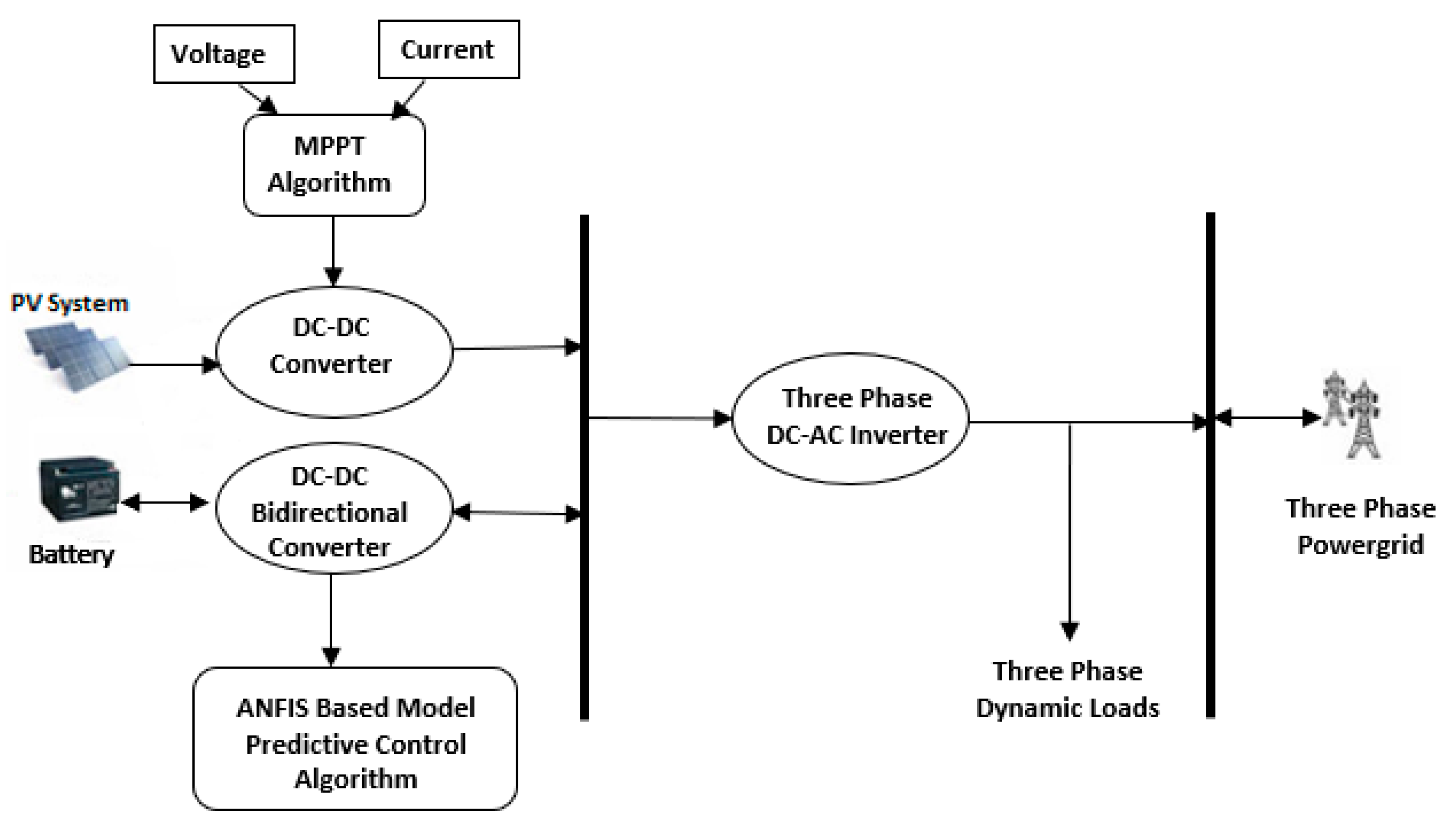
Microgrid is a small-scale power grid that has specific autonomy with its own energy resources, generation and load, which can be operated autonomous mode or connected to the grid [38]. Figure 1 shows the designed grid-connected microgrid standalone power supply system. The designed microgrid system consist of a PV system and a battery bank. All of them use DC–DC power converters in order to connect them to a central DC bus and DC–DC power converter is connected to a grid by an AC–DC three-phase rectifier.
2.1. PV System
The sun provides the Earth with more energy in one hour than the energy consumed by humans all year round [38]. For this reason, it is the renewable energy source that increases the capacity of PV systems, which is one of the renewable energy conversion systems, each year [39]. In this work eighty Sunrise Solartech SR-P660 260 PV models were used for 20 kW power generation and the each of eight serial panels connected in parallel to ten. The power–voltage and current–voltage characteristics of Sunrise Solartech SR-P660 260 PV model obtained [40].
In order to operate the PV panels more efficiently, it is necessary to know the point where maximum power is taken. Maximum power point tracking systems can be used at this point to increase the efficiency of the panel [41]. In this study, the DC–DC converter MPPT control techniques were controlled by perturb and observation algorithm [42] and the PV voltage was adapted to the DC bus voltage. The parameters of the simulation are presented in Table 1, which is taken from [40].
2.2. Batteries
In renewable energy sources, they are used as an auxiliary source for feeding loads when energy is not available from the source. It is of great importance in energy management. It reduces the negativity of the variable and unstable structure of renewable energy sources. In this work lead–acid type of battery was used for 18-kWh power store because it is usually the least expensive storage battery, providing good performance and life characteristics [43]. The battery bank rating (Ah) calculation is used the equation in (1), where the battery depth of discharge is taken as 60% [44]. In this study, battery model in Matlab/Simulink library was used.
Hence, 12 V, 125 Ah battery rating is considered. Using (1), it is worked out that the number of batteries required to connected in series was 20.
2.3. Inverters/Converters
In the designed microgrid system, the common DC bus voltage is determined as 400 V and DC–DC converter is used to increase the voltage value at the output voltage the PV system. The output power of PV system is performed by using boost type converter. The parameters of the designed converter are given in Table 2.
The output voltage of the battery is 230 V–245 V. In order to discharge the battery, it must be connected to the DA bus, for which we must increase the battery output voltage. However, at the same time in order to be able to charge the battery with the power from the DA bus, we must reduce the voltage of 400 V to the battery output voltage. Hence, the battery uses a bidirectional converter. Figure 2 shows the DC–DC bidirectional converter.
The parameters in the converter structure are expressed as Equations (2)–(4) [45,46]:
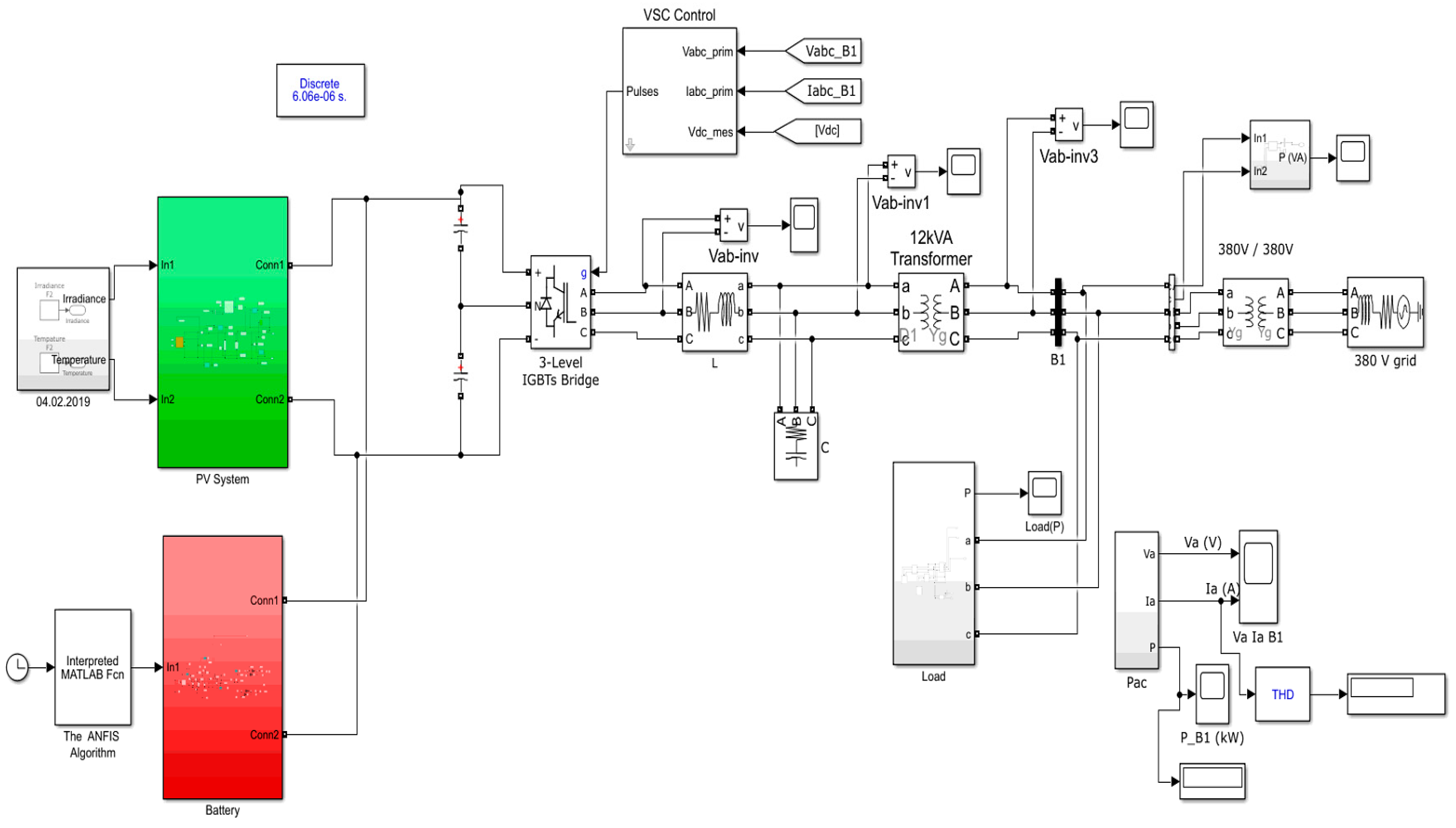
where is the battery bank voltage, is the DC-link voltage, is the DC-link current, is the battery bank current, is the buck side output desired ripple voltage, is the boost side output desired ripple voltage and is the switching frequency. The parameters of the designed DC–DC bidirectional converter are given in Table 3. Figure 3 shows the Matlab/Simulink block diagram of the designed microgrid system.
3. Microgrid Control with MPC-Inspired
3.1. Forecasting with Neural Networks
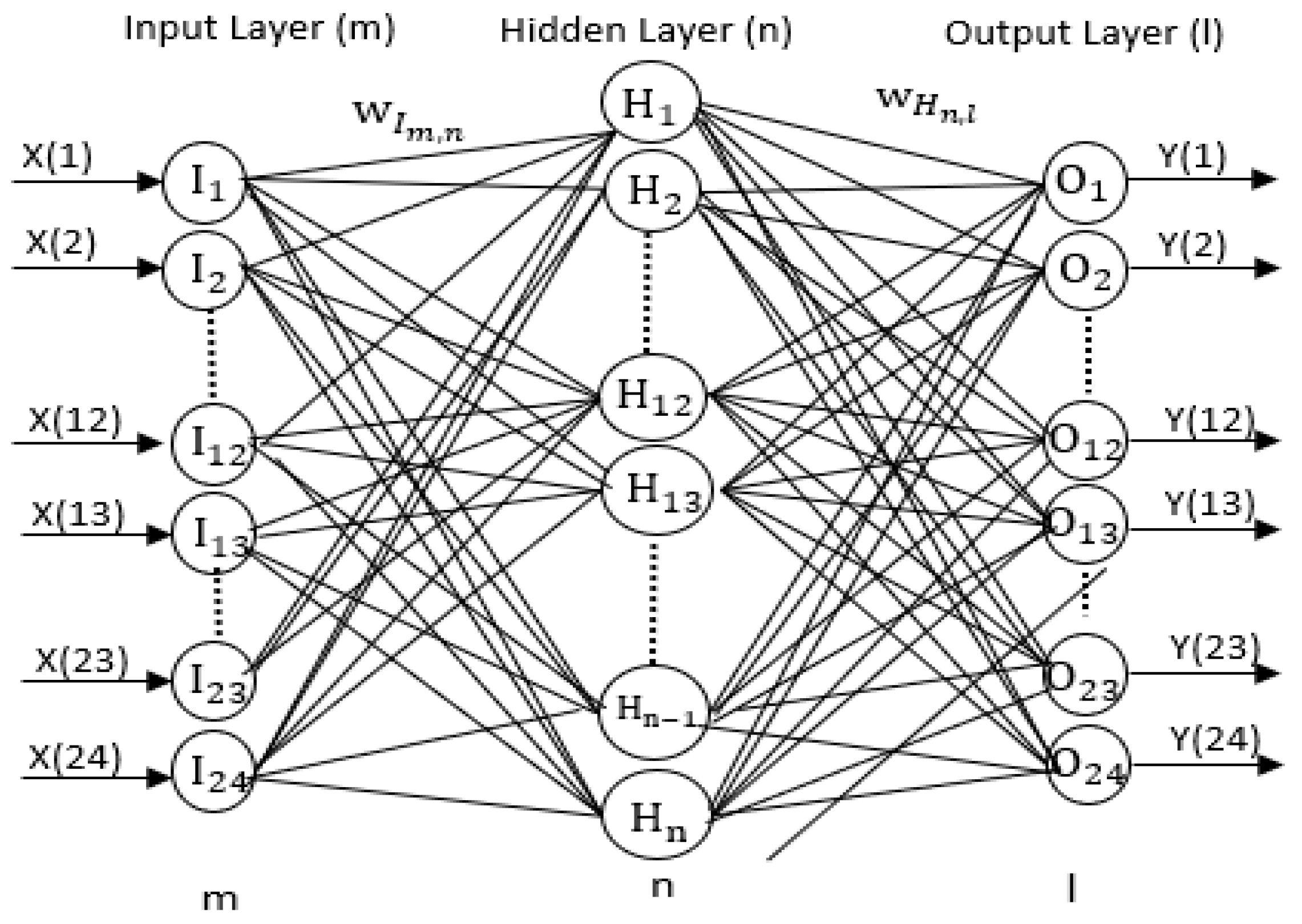
In this study, a multilayered, feed forward artificial neural network (ANN) was designed to predict the hourly solar irradiation, temperature and electricity consumption of next day in the same palace in Turkey.
In Figure 4, the structure of the multilayered ANN designed for forecasting is given. The data were normalized between 0.1–0.9 before use. In Table 4, input and output variables of ANNs designed are given. The variables X(1)–X(24) used for electricity load and temperature are the load data of the day just before the forecasting day.
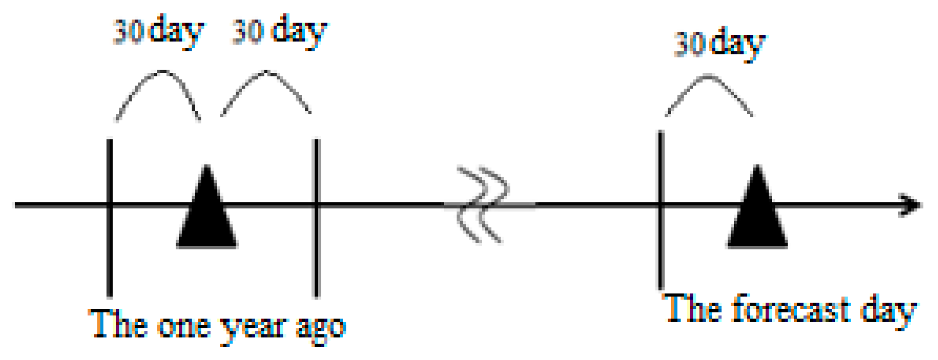
The similar day selection interval is shown in Figure 5. Since the solar irradiation, temperature and electricity loads characteristics of the seasonal effects show similarity at the same time during the year, it is considered to be a time series [47].
After selecting the 90-day interval for solar irradiation forecasting, the clearness index of each day for these 90 days was calculated and similar days were classified among themselves. Similarity was also sought between maximum temperatures. These two variables were selected by looking at the correlation between them and solar irradiation (SI). Thus, by increasing the similarity ratio, the error that will occur in the estimation was tried to be minimized. A similar day was found with the weighted Euclidean norm formed using the maximum daily temperature () and clearness index (). Similarity ratio was found with the help of Equations (5)–(7).
The effect of the parameters used for the similarity selection with the least squares method on solar irradiation was determined [48]. The determined coefficients were chosen as the most appropriate similar day by using the ratio that they affect the day irradiation in Euclidean norm. Load estimation was selected 90 days by the same interval, but 24 h load data of the previous day was used as input. In other words, only the training and testing interval selection was made with the same method.
After the 90-day training set was created, the day most like the forecast day was selected using a similar day algorithm. The 24-h data of the similar day was given as the input and the 24-h data of the forecast day was estimated as the output. Mathematically, 24-h-ahead forecasting can be formulated as Equation (8).
f is a function that finds a relationship between inputs and output data (t = 1, 2, …, 90, p = 91 and h = 24).
In this study, one-step 24-h-ahead hourly forecasting was made. Inputs are 24-hourly data to be estimated of similar day, as given in Table 5. Similar day selection is shown in Figure 5 and described in Section 3.1.
The parameters of ANN designed for solar irradiation forecasting are given in Table 6. ANN parameters were determined by try and error. Since it was observed that the error-value changed slightly when the multilayer was made, but the duration of the program was prolonged, it was decided that a single layer network was better by considering the error-value decreasing with the program time. The number of iterations and the number of neurons in the hidden layer were determined by trial and error in order to provide the highest accuracy considering the error-value (r: correlation coefficient).
Designed for load prediction, the ANN has different hidden neuron numbers and it was decided that a single layer network was better by considering the error-value decreasing with the program time. In other words, the number of layers was decided by trial and error. A total of 37 hidden neurons and 19,300 iterations were used for load estimation. The temperature forecast variables are the same as solar forecasting. Statistical performance measures such as mean absolute percent error (MAPE), correlation coefficient (r), square mean error (RMSE) and mean absolute error (MAE) were used to measure the performance of the predictions [49].
3.2. Neuro-Fuzzy Applications
The neuro-fuzzy algorithm is combining artificial neural networks (ANNs) and fuzzy logic. neuro-fuzzy systems are used in areas such as student modeling system, medical system, economic system, electrical and electronic system, traffic control [50], image processing [51] and feature extraction, production and system modeling, estimations [52], NFS developments and social sciences [53]. The adaptive neural fuzzy inference system (ANFIS) has different structures such as FuNe, fuzzy RuleNet, GARIC or NEFCLASS and NEFCON. ANFIS structure was used in this study. The aim of the neuro-fuzzy method is to apply a learning method using input-output training data and to adjust the parameters of the fuzzy system. ANFIS uses Sugeno fuzzy rules in its structure. It consists of 5 layers. Layer 1 consists of input variables. Layer 2 is a membership layer that controls the weights of the membership function. It takes input values from the first layer and membership values are specified to represent fuzzy sets of related input variables. Layer 3 is called the rule layer and takes the entries from the previous layer. This layer calculates the activation level of each rule. Layer 4 is the defuzzificated layer. It is the definition layer that provides the output values resulting from the extraction of rules. Layer 5 is the output layer that collects all inputs from the previous layer and converts the fuzzy classification results to a clear-value. In Figure 6, a typical architecture of ANFIS is shown.
3.3. Energy Management of Microgrid with Rule-Based Control
Figure 7 shows a rule-based controller (RBC) flow chart which is used to compare with the proposed neuro-fuzzy-based energy management. This is the same strategy adopted in [56] (This study has a fuel cell, so our rules are different.). The charging/discharging rate for this RBC is a constant ±6 kW. The power formulation was given in Equation (9).
3.4. Neuro-Fuzzy-Based Energy Management of Microgrid
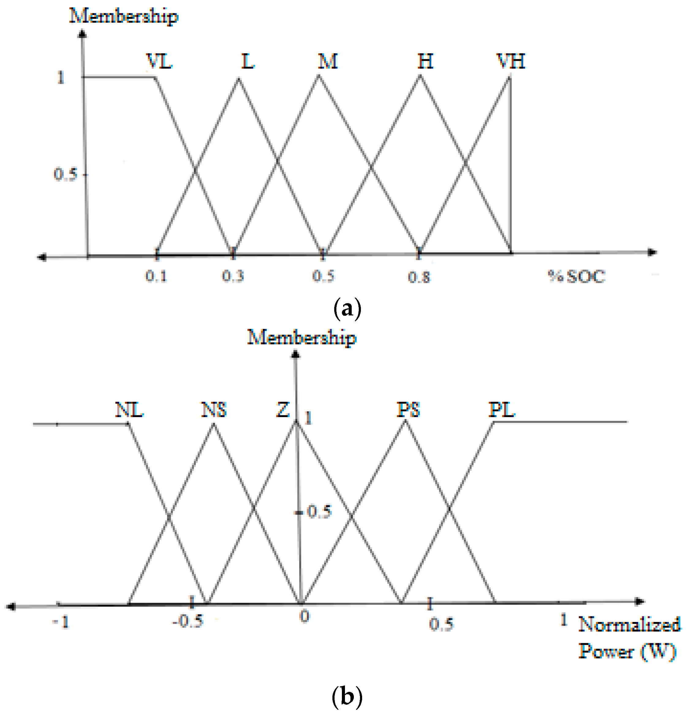
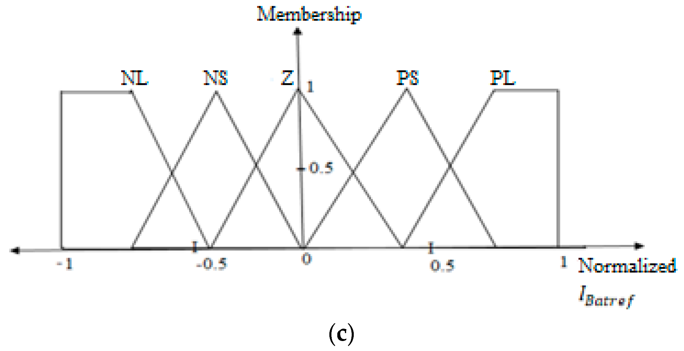
Neural networks and fuzzy are used together. In the neuro-fuzzy algorithm, energy state and battery charge rate are used as input and battery current is used as output. The limits of the inputs and outputs and the limits of membership functions are determined by trial and error. Figure 8 is shown the fuzzy clusters of inputs and outputs. fuzzy rule table is given in Table 7.
Five fuzzy values for SOC in the neuro-fuzzy rule table (VL: very low, L: low, M: medium, H: high, VH: very high), five fuzzy values for power (NL: negative large, NS: negative small, Z: zero, PS: positive small, PL: positive large) and five fuzzy values for battery reference current (NL: negative large (overcharge), NS: negative small (less charge), Z: zero, PS: positive small (less discharge), PL: positive large (very discharge)).
20% ≤ SOC ≤ 90%
25 fuzzy rules were created. The neuro-fuzzy intelligent energy management algorithm controls the power flow by making decisions based on these situations. Some of the rules used when creating the fuzzy rule table in Table 7 are given below.
- Rule 1: If the power is negative high and the SOC is very low, the is zero;
- Rule 6: If the power is negative high and SOC is low, the positive is small;
- Rule 10: If the power is positive high and the SOC is low, the is negative high;
- Rule 14: If the power is positive small and SOC is medium, the is negative small;
- Rule 22: If the power is negative small and the SOC is very high, the is positive small;
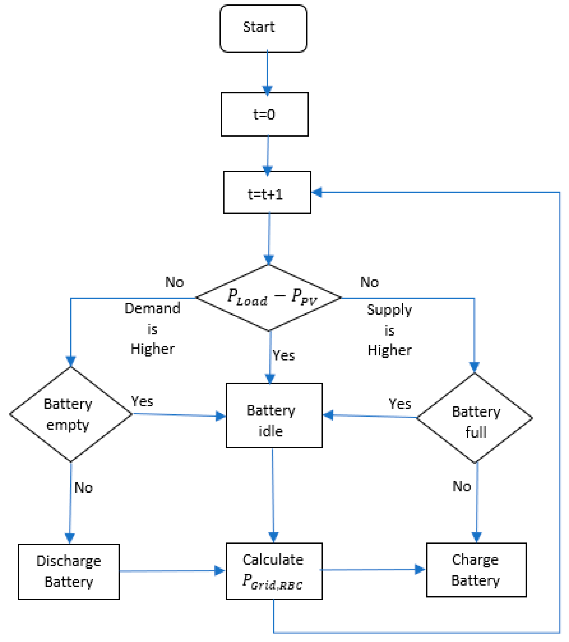
Zero fuzzy value is defined between fuzzy clusters of battery reference current so that the battery does not shorten battery life by charging or discharging for such a small value if the power generated from renewable sources is too little or too large than the load. MPC-inspired energy management algorithm flowchart is given in Figure 9.
These two energy management systems were evaluated according to the energy usage from the grid and battery discharge–charge number.
4. Results and Discussion
4.1. Results of Forecasting
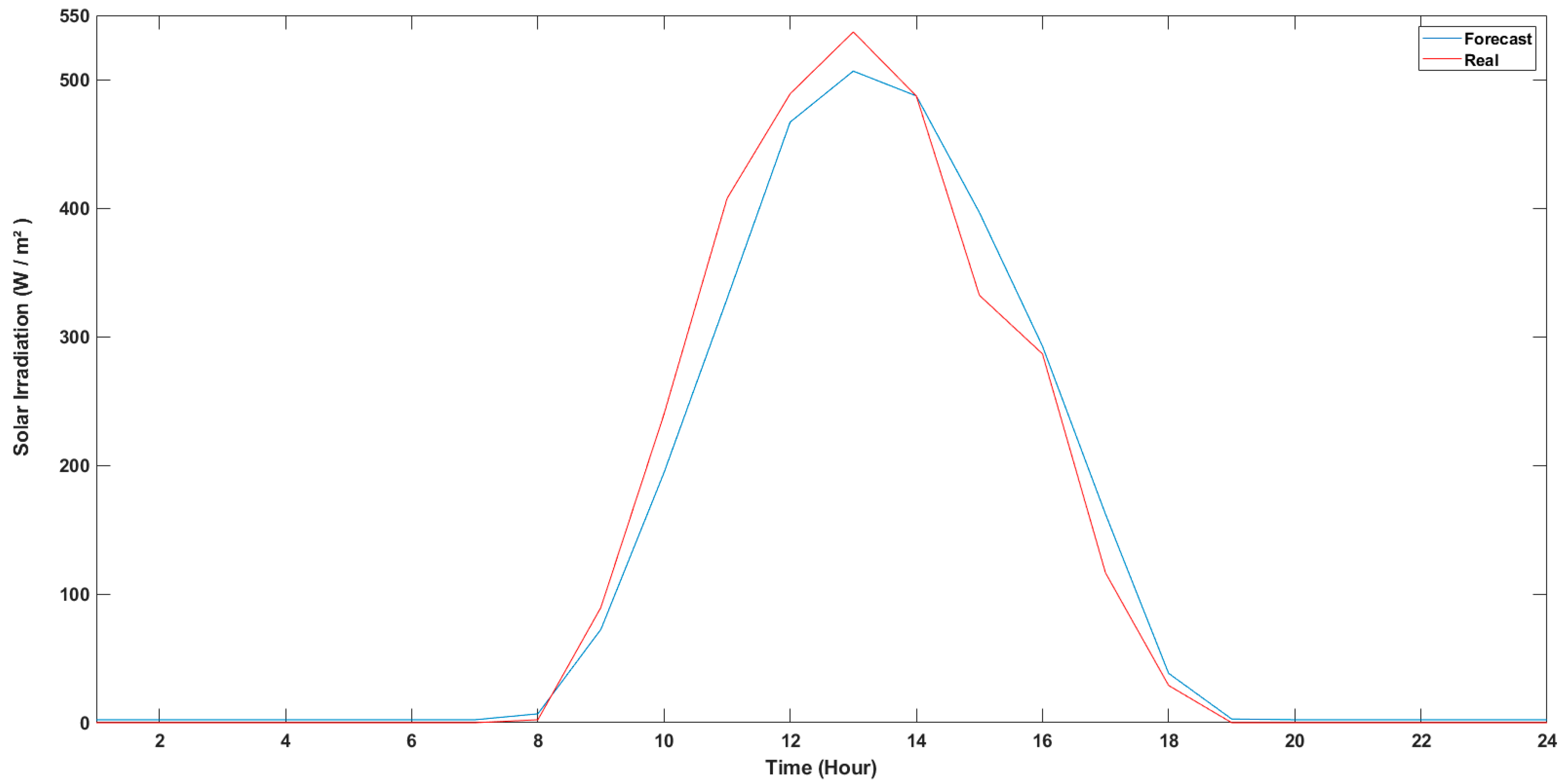
Randomly selected data refer to February 4, 2019. The hourly solar irradiation for the day of forecasting in Figure 10 was found to be 5.56% MAPE, 26.05 W/m² RMSE, 14.71 MAE and 0.9902 correlation coefficient. As the correlation coefficient approaches 1, the degree of accuracy of the estimation increases. The correlation coefficient value of 0.9902 shows us that today’s estimation is very good. Percentage error-values provide predictive results to be more meaningful and make the results easier to interpret. MAPE is the average of the sum of absolute values of percentile errors. MAPE measurement was done with normalized (0.1–0.9) values. According to the MAPE performance criterion, the estimates made under 10% are in the “high accuracy" degree, if it is between 10% and 20%, it is "true", if it is between 20% and 50%, it is "acceptable" and if it is above 50%, “false and inaccurate” [57]. Proportional or percentage error measurements are required to compare error measures. A similar day selection algorithm increased the accuracy of the prediction. High-accuracy solar irradiation estimation is performed with the designed ANN structure. The statistical performance measures for randomly selected days for 2019 were given for solar irradiation in Table 8. In this study, estimation was made with a single method and Kolmogorov–Smirnov (K–S) test applied and results are shared in Appendix C, but to test the significance of the accuracy values of two different sets of prediction, a test based on the K–S test principles, referred to as the K–S predictive accuracy (KSPA) test was proposed in [58]. 24-hourly real and forecasted data of the load, temperature and solar irradiation data from 04/02/2019 are given in Appendix B.
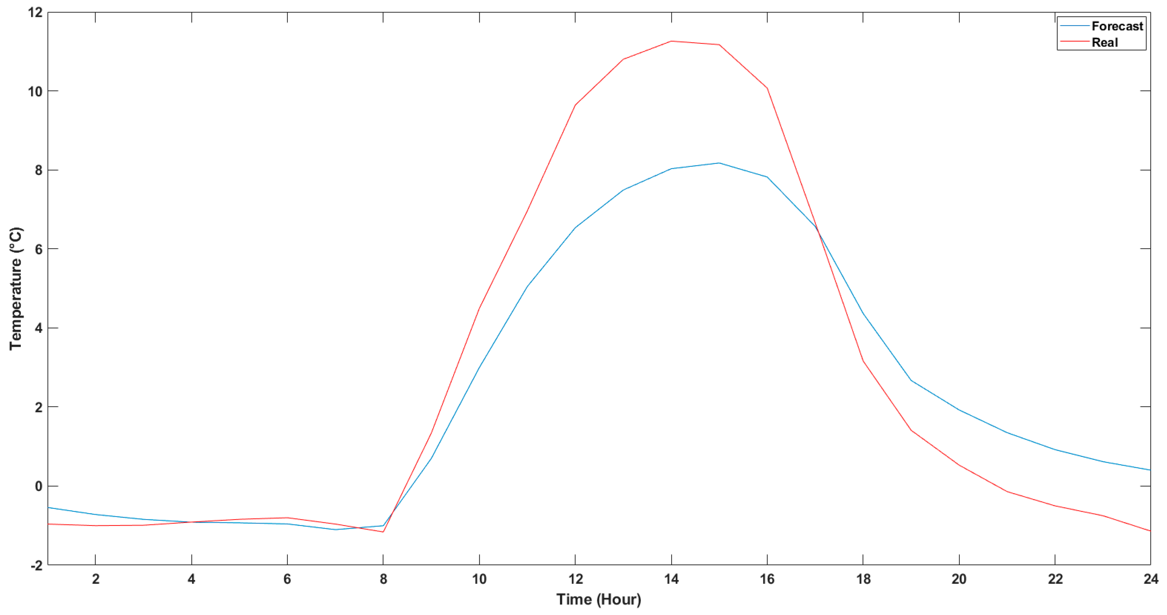
For the same day, the hourly temperature for the day of forecasting in Figure 11 was found to be 5.05% MAPE, 1.64 RMSE, 0.0262 MAE and 0.99 correlation coefficient. The correlation coefficient value of 0.99 shows us that today’s estimation is very good. High-accuracy temperature estimation is performed with the designed ANN structure. The statistical performance measures for randomly selected days for 2019 are given for temperature data in Table 9.
The forecasting temperature and solar irradiation values are given as input to the designed PV system. In addition, the actual temperature and solar irradiation values are given and the outputs in Figure 12 are obtained. The output with 0.9836 r-value.
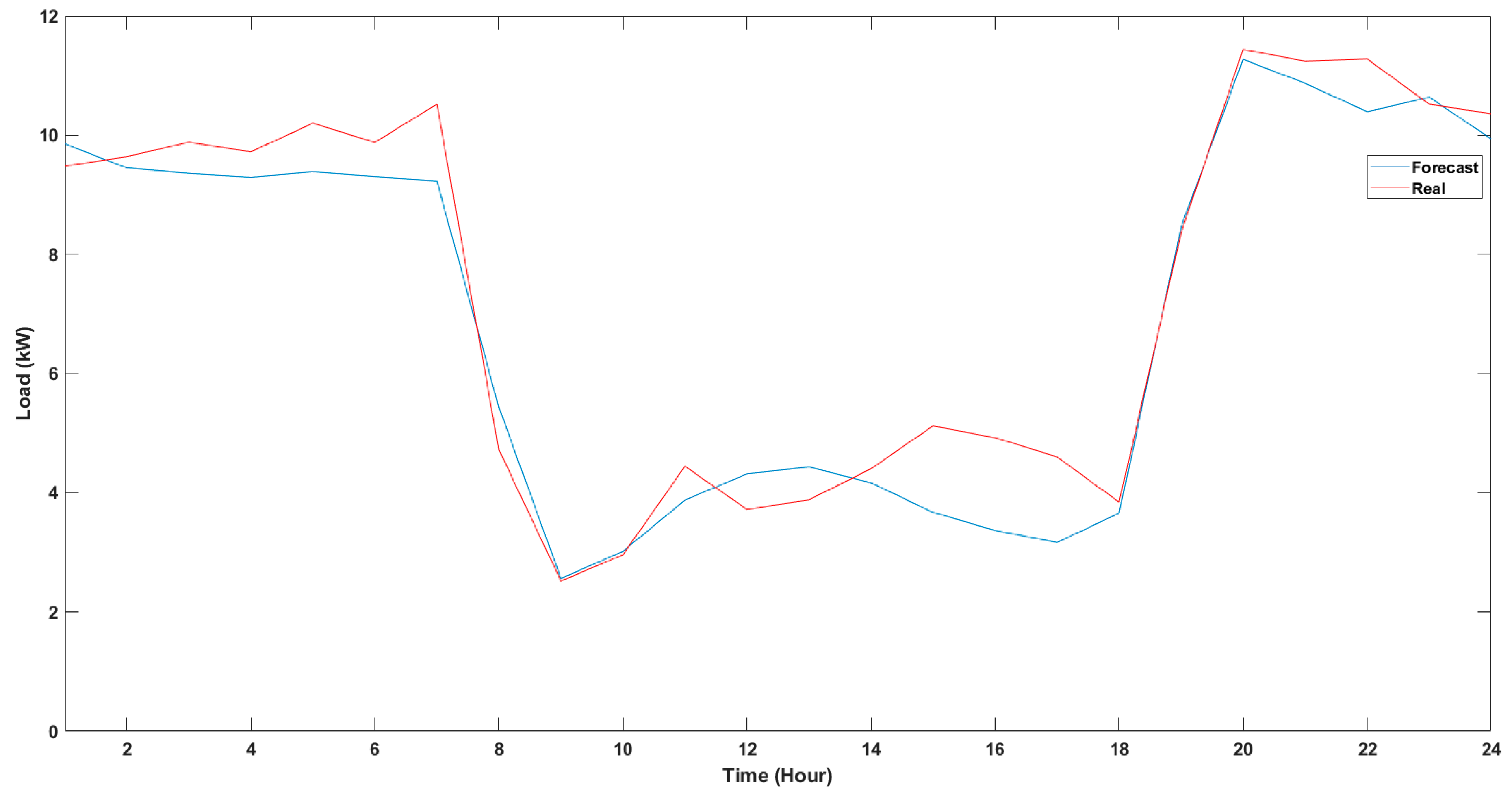
For the same day, the hourly temperature for the day of forecasting in Figure 13 was found to be 10.24% MAPE, 0.7245 RMSE, 0.0258 MAE and 0.96 correlation coefficient. The correlation coefficient value of 0.96 shows us that today’s estimation is very good. High accuracy temperature estimation is performed with the designed ANN structure. The statistical performance measures for randomly selected days for 2019 were given for load data in Table 10.
4.2. Results of Energy Management with Rule-Based Control
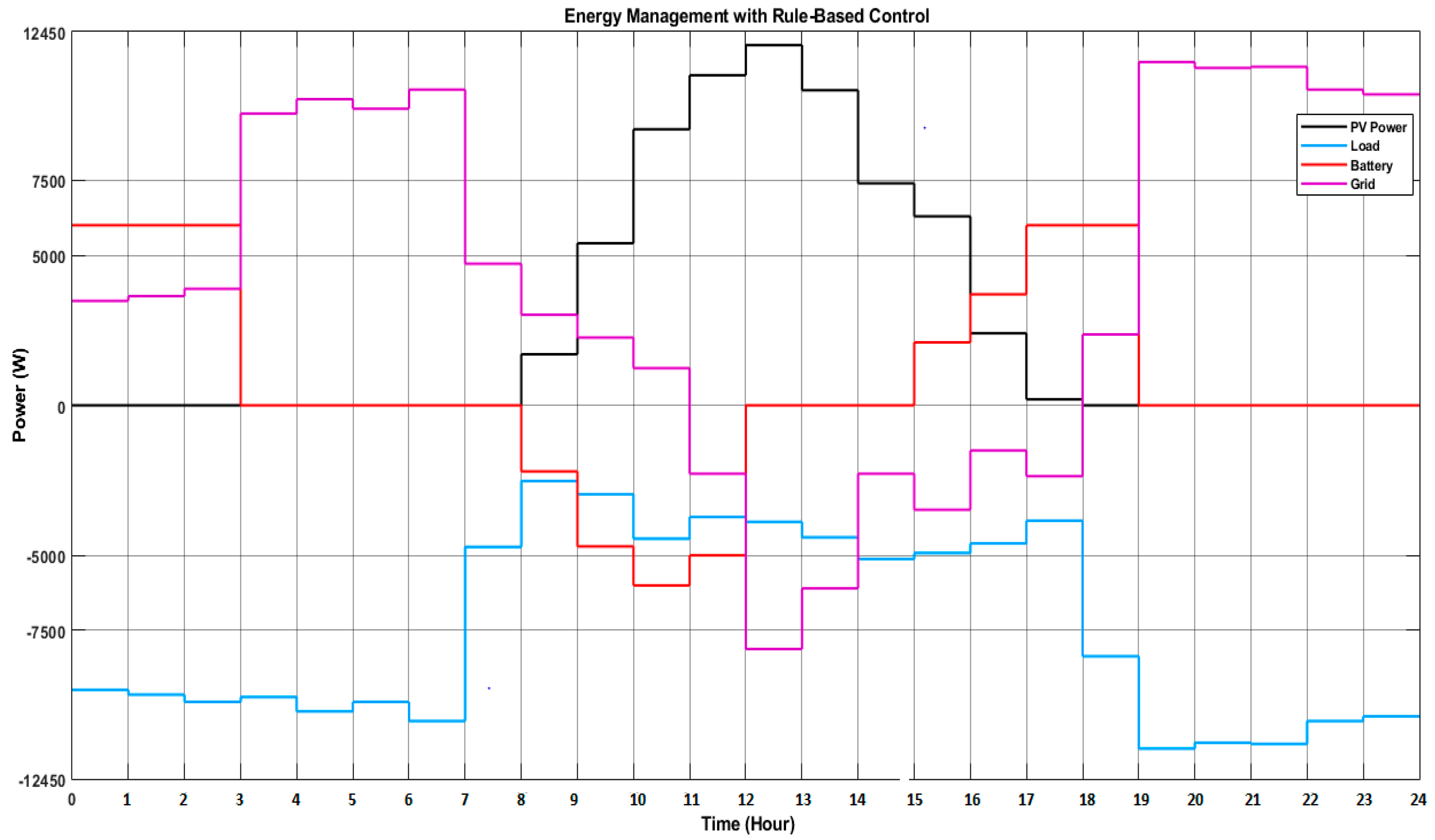
Figure 14 shows the power distribution profile with RBC for 04/02/2019.
4.3. Results of Energy Management with ANFIS-Based on MPC-Inspired
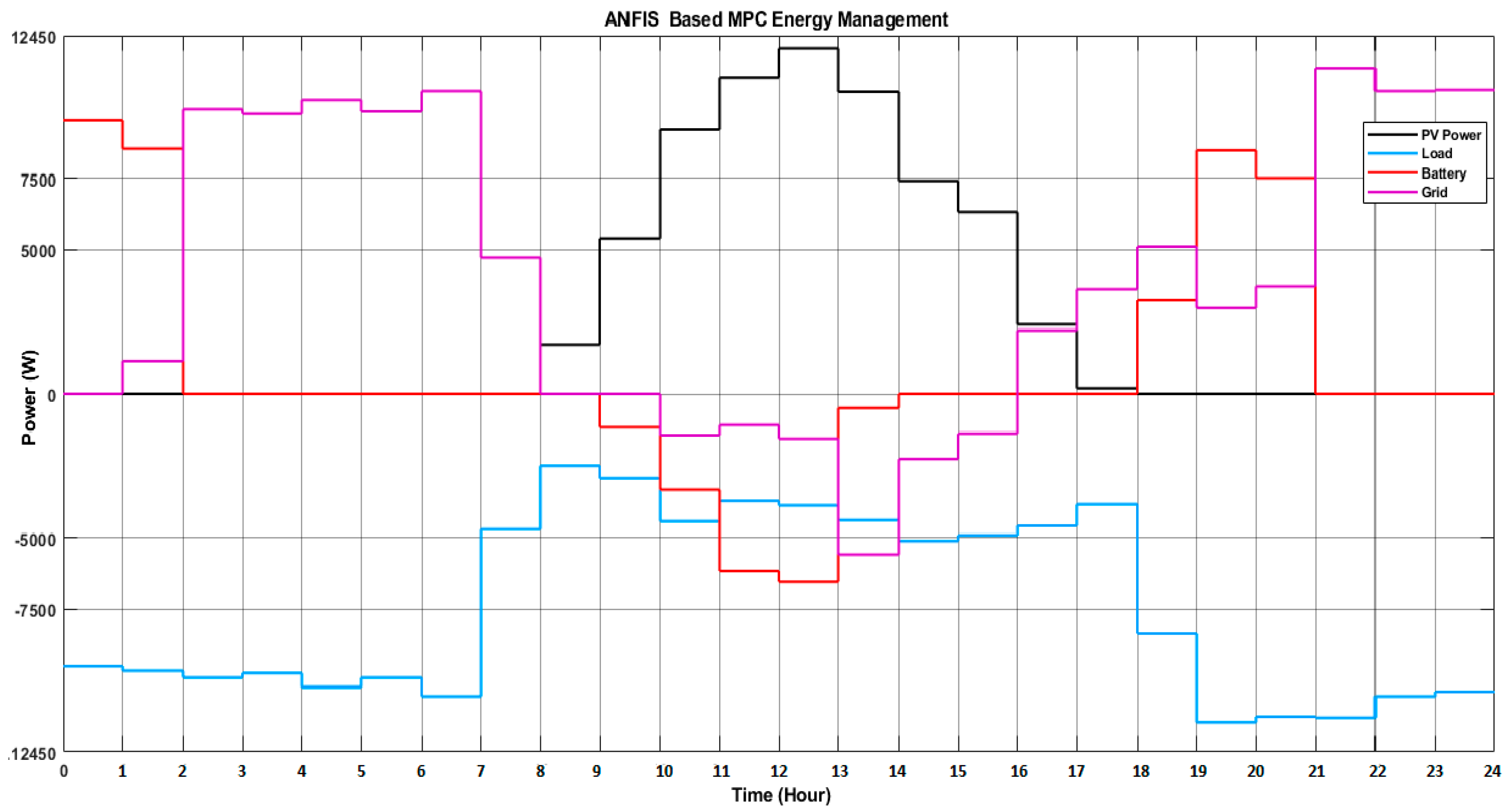
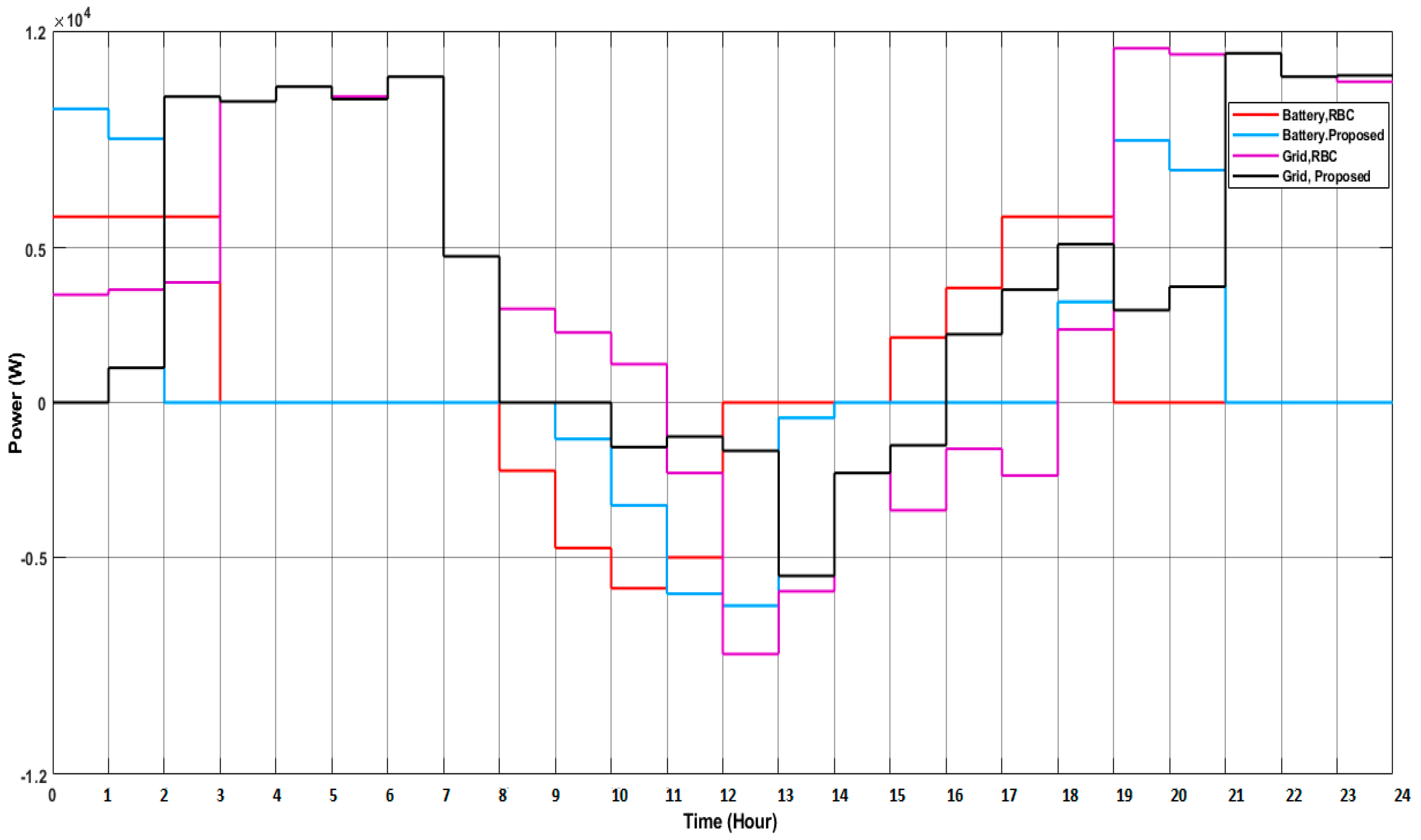
By means of this energy management, the reference voltage values to be entered for double-sided transducer control and the power-values to be drawn from the grid are determined according to the load and power generation estimation. Figure 15 shows the power distribution profile with ANFIS-based MPC-inspired for 04/02/2019. The battery is charged between 9–14 h and discharged between 18–21 h. Between 8–10 h, unused power from the grid loads are fed by PV system and battery. In Figure 16, the power used from the battery and grid are compared for both cases.
The forecasting errors on the control strategy and performance of energy management is impact. False predictions have a negative effect. For example, the PV generation was estimated to be lower than the actual value between 9–11 h. Hence, the battery is charged less than it should. Between 12–14 h PV generation was estimated to be low, electricity consumption was overestimated and excess power was drawn from the grid.
With the recommended management, it was ensured that the battery group has a longer cycle life by reducing the charge/discharge period of the battery by preventing the battery from continuously switching on and off in a small power change. For example, while the battery is not used in the management recommended between 8–9 h in Figure 16, the battery is used in the system managed by RBC. At the same time, continuous switching of the system is prevented, and power loss is reduced.
5. Conclusions
In this study, neuro-fuzzy-based MPC-inspired energy management is proposed for grid connected microgrids. Since energy production and consumption data are estimated in the recommended energy management, the model is provided with predictive control by planning energy management by the algorithm. Considering the charging status and the production estimated from the renewable source, the battery is ensured not to be de-energized and at the same time to draw as little energy from the grid as possible. With the recommended algorithm, the energy level in both devices was managed and it charge/discharge amount was decided for the battery. The proposed system is compared with a rule-based control strategy.
The proposed algorithm and ANN-prediction algorithm were implemented and the grid-connected system was simulated. The behavior of the algorithm was examined using day ahead load and PV forecast data for a specific day. The results verify that the developed energy management system predicts the load and generation with high accuracy. The grid usage is reduced with the system recommended according to RBC. Consequently, less energy exchange with the grid ensures that the bills are lower. Battery usage in the recommended system is less than RBC, so battery life is extended. With the recommended management, it was ensured that the battery group has a longer cycle life by reducing the charge/discharge period of the battery by preventing the battery from continuously switching on and off in a small power change. All these benefits encourage investors and house-owners towards use of more renewables, even if that requires some storage installation.
Author Contributions
Conceptualization, A.O. and T.S.U.; Methodology, I.H.A. and A.U.; Formal Analysis and Data Curation, A.U.; Writing, A.U., A.O., T.S.U.; Supervision, A.O. and T.S.U.; Funding Acquisition, T.S.U. All authors have read and agreed to the published version of the manuscript.
Funding
This research received no external funding.
Conflicts of Interest
The authors declare no conflict of interest.
Appendix A

Table A1.
A list of mathematical symbols.
| Symbol | Meaning |
|---|---|
| Maximum temperature of the day to be predict | |
| Maximum clearness index of the day to be predict | |
| Maximum temperature of the day investigated | |
| Maximum clearness index of the day investigated | |
| Power of battery | |
| Power of grid | |
| Voltage at the bidirectional DC–DC converter output (400 V) | |
| Forecasting of PV (W) | |
| Forecasting of load (W) | |
| Battery reference current (A) | |
| Load power (W) | |
| Correlation weight of | |
| Correlation weight of CI | |
| Power of DC central converter | |
| t | Similar day |
| p | Predicted day |
| Data to be estimated of similar day |
Appendix B
Table A2.
Forecasting results and real data for temperature and solar irritation data for 04/02/2019.
Table A2.
Forecasting results and real data for temperature and solar irritation data for 04/02/2019.
| Hour | Real Temperature (°C) | Forecasted Temperature (°C) | Real Solar Irradiation (W/m²) | Forecasted Solar Irradiation (W/m²) |
|---|---|---|---|---|
| 1 | −0.959999999999980 | −0.540086308217521 | 0 | 0 |
| 2 | −1 | −0.718577991080505 | 0 | 0 |
| 3 | −0.990000000000009 | −0.840624308071561 | 0 | 0 |
| 4 | −0.910000000000025 | −0.912112458277385 | 0 | 0 |
| 5 | −0.839999999999975 | −0.928957466784858 | 0 | 0 |
| 6 | −0.800000000000011 | −0.956741475782955 | 0 | 0 |
| 7 | −0.959999999999980 | −1.10098776218952 | 0 | 0 |
| 8 | −1.16000000000003 | −1.00182230582977 | 2.2813 | 6.895165 |
| 9 | 1.34 | 0.699430301 | 89.5956 | 72.52998 |
| 10 | 4.49 | 2.99491432 | 239.6149 | 194.2262 |
| 11 | 6.96 | 5.044016722 | 407.5313 | 329.4919 |
| 12 | 9.64 | 6.534980713 | 488.9484 | 466.8972 |
| 13 | 10.8 | 7.488420298 | 537.0333 | 506.5826 |
| 14 | 11.26 | 8.028813135 | 487.2789 | 487.2958 |
| 15 | 11.17 | 8.173712518 | 332.1361 | 396.5143 |
| 16 | 10.07 | 7.818150891 | 286.5522 | 292.5285 |
| 17 | 6.66 | 6.566347043 | 116.3132 | 161.9001 |
| 18 | 3.16 | 4.361454738 | 28.926 | 38.32243 |
| 19 | 1.41 | 2.669464139 | 0 | 0 |
| 20 | 0.53 | 1.924509355 | 0 | 0 |
| 21 | −0.139999999999986 | 1.350227131 | 0 | 0 |
| 22 | −0.500000000000000 | 0.920084749 | 0 | 0 |
| 23 | −0.750000000000000 | 0.616438286 | 0 | 0 |
| 24 | −1.13999999999999 | 0.401382591 | 0 | 0 |
Table A3.
Forecasting results and real data for load data for 04/02/2019.
| Hour | Real Load (W) | Forecasted Load (W) |
|---|---|---|
| 1 | 9.48 | 9.853449986 |
| 2 | 9.64 | 9.450117517 |
| 3 | 9.88 | 9.358285916 |
| 4 | 9.72 | 9.289548135 |
| 5 | 10.2 | 9.386478155 |
| 6 | 9.88 | 9.303034687 |
| 7 | 10.52 | 9.228701533 |
| 8 | 4.72 | 5.429989117 |
| 9 | 2.52 | 2.562437568 |
| 10 | 2.96 | 3.017490059 |
| 11 | 4.44 | 3.874763163 |
| 12 | 3.72 | 4.314246228 |
| 13 | 3.88 | 4.430281033 |
| 14 | 4.4 | 4.164480304 |
| 15 | 5.12 | 3.669769332 |
| 16 | 4.92 | 3.36645249 |
| 17 | 4.6 | 3.165261745 |
| 18 | 3.84 | 3.655727748 |
| 19 | 8.36 | 8.461599467 |
| 20 | 11.44 | 11.27290926 |
| 21 | 11.24 | 10.8710454 |
| 22 | 11.28 | 10.39287319 |
| 23 | 10.52 | 10.63655916 |
| 24 | 10.36 | 9.937350942 |
Appendix C
The first line tests the null hypothesis that load/temperature/irradiation for the first group ‘real values” contains smaller-values than for the second group “forecasted values”. The largest differences between the distribution functions are 0.250/0.208/0.041, accordingly. The approximate p-value for this is 0.223/0.353/0.959, which are not significant at an acceptable level of significance. The second line tests the hypothesis that load/temperature/irradiation for the first group ‘real values” contains larger-values than for the second group “forecasted values”. The largest differences between the distribution functions in this direction are −0.041/−0.166/−0.041. The approximate p-value for these small differences are 0.959/0.513/0.959, which are not significant either. Overall, we cannot reject the null hypothesis that these two-samples come from the same distribution.
Table A4.
Kolmogorov–Smirnov (K–S) test results.
| Load | Temperature | Irradiation | ||||
|---|---|---|---|---|---|---|
| Smaller Group | D | P-Value | D | P-Value | D | P-Value |
| Real | 0.250 | 0.223 | 0.208 | 0.353 | 0.041 | 0.959 |
| Forecast | −0.041 | 0.959 | −0.166 | 0.513 | −0.041 | 0.959 |
| Combined K–S | 0.250 | 0.441 | 0.208 | 0.675 | 0.041 | 1.000 |
References
- International Renewable Energy Agency. Global Energy Transformation: A Roadmap to 2050, 2019th ed.; International Renewable Energy Agency: Abu Dhabi, UAE, 2019. [Google Scholar]
- Electric Power Consumption (kWh per Capita)|Data. Available online: https://data.worldbank.org/indicator/EG.USE.ELEC.KH.PC?end=2018&start=1960&view=chart (accessed on 21 January 2020).
- Population without Access to Electricity Falls Below 1 Billion—Analysis—IEA. Available online: https://www.iea.org/commentaries/population-without-access-to-electricity-falls-below-1-billion (accessed on 21 January 2020).
- Hubble, A.H.; Ustun, T.S. Scaling renewable energy based microgrids in underserved communities: Latin America, South Asia, and Sub-Saharan Africa. In Proceedings of the IEEE PES PowerAfrica Conference, Lusaka, Zambia, 28 June–2 July 2016; pp. 134–138. [Google Scholar]
- Paris Agreement|Climate Action. Available online: https://ec.europa.eu/clima/policies/international/negotiations/paris_en (accessed on 10 November 2019).
- Ustun, T.S.; Nakamura, Y.; Hashimoto, J.; Otani, K. Performance analysis of PV panels based on different technologies after two years of outdoor exposure in Fukushima, Japan. Renew. Energy 2019, 136, 159–178. [Google Scholar] [CrossRef]
- Hatziargyriou, N. Microgrids: Architectures and Control; John Wiley & Sons: Hoboken, NJ, USA, 2014. [Google Scholar]
- Alam, M.S.; Arefifar, S.A. Energy management in power distribution systems: Review, classification, limitations and challenges. IEEE Access 2019, 7, 92979–93001. [Google Scholar] [CrossRef]
- Aftab, M.A.; Hussain, S.M.S.; Ali, I.; Ustun, T.S. IEC 61850 and XMPP communication based energy management in microgrids considering electric vehicles. IEEE Access 2018, 6, 35657–35668. [Google Scholar] [CrossRef]
- Ustun, T.S.; Suhail Hussain, S.S.M.C.; Kikusato, H. IEC 61850-based communication modeling of EV charge-discharge management for maximum PV generation. IEEE Access 2019, 7, 4219–4231. [Google Scholar] [CrossRef]
- Panwar, L.K.; Konda, S.R.; Verma, A.; Panigrahi, B.K.; Kumar, R. Operation window constrained strategic energy management of microgrid with electric vehicle and distributed resources. IET Gener. Transm. Distrib. 2017, 11, 615–626. [Google Scholar] [CrossRef]
- Pascual, J.; Barricarte, J.; Sanchis, P.; Marroyo, L. Energy management strategy for a renewable-based residential microgrid with generation and demand forecasting. Appl. Energy 2015, 158, 12–25. [Google Scholar] [CrossRef]
- Merabet, A.; Tawfique Ahmed, K.; Ibrahim, H.; Beguenane, R.; Ghias, A.M.Y.M. Energy management and control system for laboratory scale microgrid based wind-PV-battery. IEEE Trans. Sustain. Energy 2017, 8, 145–154. [Google Scholar] [CrossRef]
- Arcos-Aviles, D.; Pascual, J.; Guinjoan, F.; Marroyo, L.; Sanchis, P.; Marietta, M.P. Low complexity energy management strategy for grid profile smoothing of a residential grid-connected microgrid using generation and demand forecasting. Appl. Energy 2017, 205, 69–84. [Google Scholar] [CrossRef]
- Fossati, J.P.; Galarza, A.; Martín-Villate, A.; Echeverría, J.M.; Fontán, L. Optimal scheduling of a microgrid with a fuzzy logic controlled storage system. Int. J. Electr. Power Energy Syst. 2015, 68, 61–70. [Google Scholar] [CrossRef]
- Prodan, I.; Zio, E. A model predictive control framework for reliable microgrid energy management. Int. J. Electr. Power Energy Syst. 2014, 61, 399–409. [Google Scholar] [CrossRef]
- Minchala-Avila, L.I.; Garza-Castanon, L.; Zhang, Y.; Ferrer, H.J.A. Optimal energy management for stable operation of an islanded microgrid. IEEE Trans. Ind. Inform. 2016, 12, 1361–1370. [Google Scholar] [CrossRef] [Green Version]
- Zia, M.F.; Elbouchikhi, E.; Benbouzid, M. Microgrids energy management systems: A critical review on methods, solutions, and prospects. Appl. Energy 2018, 222, 1033–1055. [Google Scholar] [CrossRef]
- Bruni, G.; Cordiner, S.; Mulone, V.; Rocco, V.; Spagnolo, F. A study on the energy management in domestic micro-grids based on model predictive control strategies q. Energy Convers. Manag. 2015, 102, 50–58. [Google Scholar] [CrossRef]
- Mahmud, N.; Zahedi, A.; Mahmud, A. A cooperative operation of novel PV inverter control scheme and storage energy management system based on ANFIS for voltage regulation of grid-tied PV system. IEEE Trans. Ind. Inform. 2017, 13, 2657–2668. [Google Scholar] [CrossRef]
- Hasaranga, W.V.H.; Hemarathne, R.D.T.M.; Mahawithana, M.D.C.P.K.; Sandanuwan, M.G.A.B.N.; Hettiarachchi, H.W.D.; Hemapala, K.T.M.U. A Fuzzy logic based battery SOC level control strategy for smart Micro grid. In Proceedings of the 2017 Third International Conference on Advances in Electrical, Electronics, Information, Communication and Bio-Informatics, (AEEICB), TamilNadu, India, 27–28 Feburary 2017; pp. 215–221. [Google Scholar]
- Teo, T.T.; Logenthiran, T.; Woo, W.L.; Abidi, K. Fuzzy logic control of energy storage system in microgrid operation. In Proceedings of the 2016 IEEE Innovations Smart Grid Technologies—Asia, Melbourne, Australia, 28 November–1 December 2016; pp. 65–70. [Google Scholar]
- Küçüker, A.; Kamal, T.; Hassan, S.Z.; Li, H.; Mufti, G.M.; Waseem, M.H. Design and control of photovoltaic/wind/battery based microgrid system. In Proceedings of the 2017 International Conference on Electrical Engineering (ICEE), Lahore, Pakistan, 2–4 March 2017; pp. 1–6. [Google Scholar]
- Roldán-Blay, C.; Escrivá-Escrivá, G.; Roldán-Porta, C.; Álvarez-Bel, C. An optimisation algorithm for distributed energy resources management in micro-scale energy hubs. Energy 2017, 132, 126–135. [Google Scholar] [CrossRef]
- Mbungu, N.T.; Naidoo, R.; Bansal, R.C.; Bipath, M. Optimisation of grid connected hybrid photovoltaic-wind-battery system using model predictive control design. IET Renew. Power Gener. 2017, 11, 1760–1768. [Google Scholar] [CrossRef]
- De Santis, E.; Rizzi, A.; Sadeghian, A. Hierarchical genetic optimization of a fuzzy logic system for energy flows management in microgrids. Appl. Soft Comput. J. 2017, 60, 135–149. [Google Scholar] [CrossRef] [Green Version]
- Chettibi, N.; Mellit, A.; Sulligoi, G.; Member, I.S.; Pavan, A.M.; Member, I. Adaptive neural network—Based Control of a Hybrid AC/DC Microgrid. IEEE Trans. Smart Grid 2016, 9, 1667–1679. [Google Scholar] [CrossRef] [Green Version]
- Elgammal, A.; El-Naggar, M. Energy management in smart grids for the integration of hybrid wind–PV–FC–battery renewable energy resources using multi-objective particle swarm optimisation (MOPSO). J. Eng. 2018, 2018, 1806–1816. [Google Scholar] [CrossRef]
- Hussain, A.; Bui, V.H.; Kim, H.M. A resilient and privacy-preserving energy management strategy for networked microgrids. IEEE Trans. Smart Grid 2018, 9, 2127–2139. [Google Scholar] [CrossRef]
- Jafari, M.; Malekjamshidi, Z.; Lu, D.D.C.; Zhu, J. Development of a fuzzy-logic-based energy management system for a multiport multioperation mode residential smart microgrid. IEEE Trans. Power Electron. 2019, 34, 3283–3301. [Google Scholar] [CrossRef]
- Lee, J.; Zhang, P.; Gan, L.K.; Howey, D.A.; Osborne, M.A.; Tosi, A.; Duncan, S. Optimal operation of an energy management system using model predictive control and Gaussian process time-series modeling. IEEE J. Emerg. Sel. Top. Power Electron. 2018, 6, 1783–1795. [Google Scholar] [CrossRef]
- Bordons, C.; Garcia-Torres, F.; Ridao, M. Model. Predictive Control of Microgrids; Springer: Berlin/Heidelberg, Germany, 2020. [Google Scholar]
- Mayne, D.Q.; Rawlings, J.B.; Rao, C.V.; Scokaert, P.O.M. Constrained model predictive control: Stability and optimality. Automatica 2000, 36, 789–814. [Google Scholar] [CrossRef]
- Findeisen, R.; Allgower, F. An introduction to nonlinear model predictive control. In Benelux Meeting on Systems and Control; Technische Universiteit Eindhoven Veldhoven: Eindhoven, The Netherlands, 2002. [Google Scholar]
- Maciejowski, J.M. Predictive Control with Constraints; Prentice Hall: Upper Saddle River, NJ, USA, 2001. [Google Scholar]
- Glavic, M.; Van Cutsem, T. Some Reflections on Model. Predictive Control of Transmission Voltages; North American Power Symposium: Carbondale, IL, USA, 2006. [Google Scholar]
- Parisio, A.; Rikos, E.; Glielmo, L. Stochastic model predictive control for economic/environmental operation management of microgrids: An experimental case study. J. Process. Control 2016, 43, 24–37. [Google Scholar] [CrossRef] [Green Version]
- Mariam, L.; Basu, M.; Conlon, M.F. A review of existing microgrid architectures. J. Eng. 2013, 2013, 937614. [Google Scholar] [CrossRef] [Green Version]
- Lewis, N.S.; Nocera, D.G. Powering the planet: Chemical challenges in solar energy utilization. In Proceedings of the National Academy of Sciences of the United States of America, Paris, France, 21–24 October 2006; Volume 103, pp. 15729–15735. [Google Scholar]
- Renewables 2018 Global Status Report. Available online: https://www.ren21.net/wp-content/uploads/2019/08/Full-Report-2018.pdf (accessed on 20 November 2019).
- Sunrise|SR-P660 260-285|Solar Panel Datasheet|ENF Panel Directory. Available online: https://www.enfsolar.com/pv/panel-datasheet/crystalline/30542 (accessed on 23 November 2019).
- Masoum, M.A.; Dehbonei, S.H.; Fuchs, E.F. Theoretical and experimental analyses of photovoltaic systems with voltage- and current-based maximum power-point tracking. IEEE Trans. Energy Convers. 2002, 17, 514–522. [Google Scholar] [CrossRef] [Green Version]
- Femia, N.; Petrone, G.; Spagnuolo, G.; Vitelli, M. Optimizing duty-cycle perturbation of P&O MPPT technique. In Proceedings of the PESC Record—IEEE Annual Power Electronics Specialists Conference, Aachen, Germany, 20–25 June 2004; Volume 3, pp. 1939–1944. [Google Scholar]
- Linden, D.; Reddy, T.B. Handbook of Batteries; McGraw-Hill: New York, NY, USA, 2002. [Google Scholar]
- IEEE Guide for the Selection and Sizing of Batteries for Uninterruptible Power Systems. In IEEE Std 1184–1994; IEEE: Piscataway, NJ, USA, 6 June 1995.
- Green, M. Application Report Design Calculations for Buck-Boost Converters; Texas Instruments: Dallas, TX, USA, 2012. [Google Scholar]
- Haruni, A. A Stand-Alone Hybrid Power System with Energy Storage. Ph.D. Thesis, University of Tasmania, Hobart, Australia, 2013. [Google Scholar]
- Senjyu, T.; Sakihara, H.; Tamaki, Y.; Uezato, K. Next-day load curve forecasting using neural network based on similarity. Electr. Power Compon. Syst. 2001, 29, 939–948. [Google Scholar]
- Ulutaş, A.; Çakmak, R.; Altaş, I.H. Hourly solar irradiation prediction by artificial neural network based on similarity analysis of time series. In Proceedings of the 2018 Innovations in Intelligent Systems and Applications Conference, Madeira Island, Portugal, 25–27 September 2018. [Google Scholar]
- Stone, R.J. Improved statistical procedure for the evaluation of solar radiation estimation models. Sol. Energy 1993, 51, 289–291. [Google Scholar] [CrossRef]
- Abdennour, A.A. Long horizon neuro-fuzzy predictor for MPEG video traffic. J. King Saud Univ. Eng. Sci. 2005, 18, 161–179. [Google Scholar] [CrossRef]
- Ioannou, S.V.; Raouzaiou, A.T.; Tzouvaras, V.A.; Mailis, T.P.; Karpouzis, K.C.; Kollias, S.D. Emotion recognition through facial expression analysis based on a neurofuzzy network. Neural Netw. 2005, 18, 423–435. [Google Scholar] [CrossRef]
- Chen, C.W. Modeling, control, and stability analysis for time-delay TLP systems using the fuzzy Lyapunov method. Neural Comput. Appl. 2011, 20, 527–534. [Google Scholar] [CrossRef]
- Kar, S.; Das, S.; Ghosh, P.K. Applications of neuro fuzzy systems: A brief review and future outline. Appl. Soft Comput. J. 2014, 15, 243–259. [Google Scholar] [CrossRef]
- Jang, J.S.R.; Sun, C.T. Neuro-fuzzy modeling and control. Proc. IEEE 1995, 83, 378–406. [Google Scholar] [CrossRef]
- Bruni, G.; Cordiner, S.; Mulone, V. Domestic distributed power generation: Effect of sizing and energy management strategy on the environmental efficiency of a photovoltaic-battery-fuel cell system. Energy 2014, 77, 133–143. [Google Scholar] [CrossRef]
- Lewis, C.D. Industrial and Business Forecasting Methods; Butterworths Publishing: London, UK, 1982. [Google Scholar]
- Hassani, H.; Silva, E. A kolmogorov-smirnov based test for comparing the predictive accuracy of two sets of forecasts. Econometrics 2015, 3, 590–609. [Google Scholar] [CrossRef] [Green Version]
Figure 1.
Structure of the designed microgrid system.

Figure 2.
Structure of the DC–DC bidirectional converter.

Figure 3.
Matlab/Simulink block diagram of the designed microgrid system.

Figure 4.
The structure of the designed artificial neural network (ANN).

Figure 5.
The similar day selection interval [47].
Figure 5.
The similar day selection interval [47].


Figure 7.
Rule-based control flowchart [56].
Figure 7.
Rule-based control flowchart [56].

Figure 8.
The fuzzy sets of (a) SoC (state of charge), (b) power and (c) battery current.


Figure 9.
MPC-inspired energy management algorithm flowchart.

Figure 10.
Forecasting and real solar irradiation curves for 04/02/2019.

Figure 11.
Forecasting and real temperature curves for 04/02/2019.

Figure 12.
Forecasting and real PV power curves for 04/02/2019.

Figure 13.
Forecasting and real load curves for 04/02/2019.

Figure 14.
Power dispatching using energy management with rule-based controller (RBC) for 04/02/2019.
Figure 14.
Power dispatching using energy management with rule-based controller (RBC) for 04/02/2019.

Figure 15.
Power dispatching using with ANFIS-based MPC-inspired energy management for 04/02/2019.

Figure 16.
Comparison of battery usage and grid usage.

Table 1.
PV (photovoltaic) model parameters.
| Module | |
|---|---|
| Maximum rated power () | 260 W |
| Maximum voltage () | 30.61 V |
| Maximum current () | 8.5 A |
| Open circuit voltage () | 37.89 V |
| Shot circuit voltage () | 9.08 A |
| Array | |
| No. of modules in parallel | 10 |
| No. of modules in series | 8 |
Table 2.
DC–DC boost converter parameters.
| Parameters | Value |
|---|---|
| Input voltage () | 200–270 V |
| Inductance (L) | 1.2661 mH |
| Capacitance (C) | 0.05935 |
| Output voltage () | 400 V |
| Load (R) | 21.35 |
| Frequency of switches (f) | 5000 Hz |
| Ripple of inductance current ( | 30% |
| Ripple of capacitance voltage ( | 1% |
Table 3.
DC–DC bidirectional converter parameters.
| The Parameters | Value |
|---|---|
| V | 230 V–245 V |
| 400 V | |
| 6 kW | |
| f | 5 kHz |
| 2.304 mH | |
| 0.260 | |
| 100 |
Table 4.
Input and output variables of ANN.
| Input Variables | Explanation |
|---|---|
| X(1)–X(24) | Hourly data to be estimated of similar day (W/m²) |
| Output Variables | Explanation |
| Y(1)–Y(24) | Hourly data to be estimated for the day to be forecasted (W/m²) |
Table 5.
One-step-ahead prediction methods.
| Forecasting | Inputs |
|---|---|
Table 6.
Parameters of ANN designed for solar irradiation forecasting.
| The Name of Variables | Solar Irradiation |
|---|---|
| The number of inputs | 24 |
| The number of outputs | 24 |
| Hidden layer | 1 |
| Activation function | Logistic sigmoid function |
| Training algorithm | Backpropagation algorithm |
| The number of neurons in hidden layer | 29 |
| The number of iterations | 63,000 |
Table 7.
Fuzzy rule table.
| SOC | Power (()W) | |||||
| NL | NS | Z | PS | PH | ||
| VL | Z | Z | Z | NS | NL | |
| (1) | (2) | (3) | (4) | (5) | ||
| L | PS | Z | Z | NS | NL | |
| (6) | (7) | (8) | (9) | (10) | ||
| M | PL | PL | Z | NS | NL | |
| (11) | (12) | (13) | (14) | (15) | ||
| H | PL | PS | Z | Z | NS | |
| (16) | (17) | (18) | (19) | (20) | ||
| VH | PL | PS | Z | Z | Z | |
| (21) | (22) | (23) | (24) | (25) | ||
Table 8.
Statistical performance measures for solar irradiation.
| Date | MAPE | RMSE (W/m²) | MAE | r |
|---|---|---|---|---|
| 10.04.2019 | 6.9979% | 98.3127 | 43.5547 | 0.9672 |
| 23.06.2019 | 4.31% | 46.6757 | 26.258884 | 0.9951 |
| 28.09.2019 | % 7.1321 | 47.3810 | 31.6013 | 0.9972 |
Table 9.
Statistical performance measures for temperature.
| Date | MAPE | RMSE | MAE | r |
|---|---|---|---|---|
| 10.04.2019 | 5.9947% | 0.6637 | 0.174 | 0.9682 |
| 23.06.2019 | 6.0332% | 2.4403 | 0.232 | 0.9117 |
| 28.09.2019 | % 9.3468 | 2.2917 | 0.0319 | 0.8816 |
Table 10.
Statistical performance measures for load data.
| Date | MAPE | RMSE | MAE | r |
|---|---|---|---|---|
| 10.04.2019 | 9.4018% | 0.6160 | 0.0476 | 0.9847 |
| 23.06.2019 | 5.9547% | 0.8208 | 0.0261 | 0.9803 |
| 28.09.2019 | % 3.4242 | 3.9698 | 0.0178 | 0.9948 |
© 2020 by the authors. Licensee MDPI, Basel, Switzerland. This article is an open access article distributed under the terms and conditions of the Creative Commons Attribution (CC BY) license (http://creativecommons.org/licenses/by/4.0/).
Share and Cite
MDPI and ACS Style
Ulutas, A.; Altas, I.H.; Onen, A.; Ustun, T.S. Neuro-Fuzzy-Based Model Predictive Energy Management for Grid Connected Microgrids. Electronics 2020, 9, 900. https://doi.org/10.3390/electronics9060900
AMA Style
Ulutas A, Altas IH, Onen A, Ustun TS. Neuro-Fuzzy-Based Model Predictive Energy Management for Grid Connected Microgrids. Electronics. 2020; 9(6):900. https://doi.org/10.3390/electronics9060900
Chicago/Turabian StyleUlutas, Ahsen, Ismail Hakki Altas, Ahmet Onen, and Taha Selim Ustun. 2020. "Neuro-Fuzzy-Based Model Predictive Energy Management for Grid Connected Microgrids" Electronics 9, no. 6: 900. https://doi.org/10.3390/electronics9060900
Note that from the first issue of 2016, this journal uses article numbers instead of page numbers. See further details here.