Prediction of Temperature Distribution for Previous Cement Concrete Pavement with Asphalt Overlay


1
School of Civil Engineering and Transportation, South China University of Technology, Guangzhou 510640, China
2
Key Laboratory of Road Structure & Material Ministry of Transport, Chang’an University, Xi’an 710064, China
*
Author to whom correspondence should be addressed.
Appl. Sci. 2020, 10(11), 3697; https://doi.org/10.3390/app10113697
Submission received: 11 April 2020
/
Revised: 15 May 2020
/
Accepted: 20 May 2020
/
Published: 27 May 2020
(This article belongs to the Special Issue Asphalt Materials II)
Abstract
:In this study, the temperature distribution of a pavement was predicted by developing an analytic algorithm. The Laplace and inverse Laplace transform techniques and Gaussian quadratic formula were applied to a pavement system of an asphalt overlay placed over an existing concrete pavement. The temperature distribution of the previous cement concrete pavement with an asphalt overlay can be estimated with the proposed analytical method regardless of the depth and time. To conduct the method, the layer thicknesses, material thermal properties and climatic factors (including air temperature, wind velocity and solar radiation) were firstly input. Then, a discrete least-squares approximation of the interpolatory trigonometric polynomials was used to fit some specific measured climatic factors considered in the surface boundary condition, i.e., the measured solar radiation intensity and air temperature. The pavement surface convection coefficient can be approximately calculated by the wind speed. The temperature solutions are validated with the measured pavement temperature data of two different periods of a whole year (summer and winter). The obtained results demonstrate the feasibility of the developed analytical approach to predict the temperature distribution of the existing cement concrete pavement with an asphalt overlay in different weather conditions with acceptable accuracy.
1. Introduction
Asphalt overlays can be used for reconstruction on existing cement concrete pavements, due to their good asphalt pavement performance, easy construction, lesser environmental pollution and property of being driven on comfortably. To accurately design an asphalt overlay, understand the asphalt material’s behavior and predict the pavement performance, it is necessary to predict the alteration of the pavement temperature with the time and depth in a pavement system of an asphalt overlay placed over an existing concrete pavement. Climatic conditions (including air temperature, wind velocity and solar radiation) and the pavement material’s thermal properties affect critically the pavement temperature distribution. Empirical, analytical and numerical models are generally developed in predicting the pavement temperature distribution [1]. The increasing numbers of analytical methods have been developed and conducted to solve the partial differential equation of heat transfer, mainly including the separation variable method, Hankel integral transform method, Laplace transform and Laplace inverse transform, Green’s function, finite integral transform and the eigenfunction expansion technique, among others.
The solving of the heat conduction problem associated with the initial boundary value can usually lead to analytical solutions of the pavement temperature. Based on a one-layer system, a closed-form solution for the maximum temperature at various depths to this problem was firstly presented by Barber [2]. With a simplified boundary condition, a similar method based on a three-layer system was subsequently presented by Liang and Niu [3]. With a one-dimensional temperature profile, a closed-form solution was also obtained in a whole time period by assuming known pavement surface temperatures by Liu and Yuan [4]. Dynamic temperature profiles of a two-layered pavement system under site conditions were determined by Chong et al. [5] using the numerical Laplace and inverse Laplace transforms.
In a multilayered pavement system, the prediction of a two-dimensional axisymmetric temperature field was obtained through building this theoretical solution. According to the research of Wang and Roesler, an analytical solution of a one-dimensional temperature profile prediction with the use of the separation of variables method was proposed in two different types of multilayered pavement systems including rigid pavement [6] and asphalt pavement [7]. Wang et al. [8] developed the Hankel integral transform method to derive the theoretical solution of the temperature field in a multilayered pavement system, where the measured air temperatures and solar radiation intensities were fitted by the interpolatory trigonometric polynomials based on discrete Fourier transform. The Laplace transform method was also utilized to predict a one-dimensional temperature profile in an N-layered rigid pavement system by Wang and Roesler [9]. Then, an algorithm was presented by neglecting the effect of climatic data and using Laplace transform based on the measured surface temperature data [10]. Furthermore, Wang developed Duhamel’s principle [7], the eigenfunction expansion technique [11], and the odd extension method [12] in deriving the analytical solution of predicting the time-dependent temperature field separately. Further, Chen et al. proposed the temperature field analytical solution in the application of a multilayered pavement structure with the Green’s function method [13,14]. According to Alawi et al. [15], a mathematical model was used to predict the temperature distribution by addressing nonlinear heat diffusion issues of pavement spherical roads with the finite integral transform method.
Without aiming to the solutions of the partial differential equation for heat conduction, Qin [16] presented a theoretical model to predict the pavement surface temperature and the model incorporated the pavement thermal properties, the surface, albedo, and the daily zenith incident solar irradiation. Further, on the basis of a simplified energy balance at the pavement surface, Dumais and Dore [17] proposed a pavement surface temperature model as a function of albedo. According to some empirical assumptions, the above mentioned models available to some specific conditions can be conducted.
The objective of this study is to predict the temperature distribution in a pavement system of an asphalt overlay placed over an existing concrete pavement by developing an analytical solution using Laplace and inverse Laplace transform, in which, a time-dependent one-dimensional mathematical temperature model of pavement under a natural environment is deduced by the heat conduction theory. The use of a discrete least-squares approximation of the interpolatory trigonometric polynomials was selected to fit the data including the measured solar radiation intensity and air temperatures. The pavement surface convection coefficient can be approximately calculated by the wind speed. The deduction on the relationship between the first layer and the constants of integration for the jth layer was simply conducted, and the temperature field in the existing cement concrete pavement with an asphalt overlay was solved by a Gaussian quadratic formula used in the numerical evaluation of the inverse Laplace transform. The temperature solutions are validated with the measured temperature field data from the existing cement concrete pavement with an asphalt overlay.
2. Mathematical Model of Pavement Temperature Field
2.1. Governing Equation
The time-dependent one-dimensional temperature function of the jth layer in an n-layered existing cement concrete pavement with asphalt overlay is assumed to be , which varies with the depth (z) and time (t). The material is considered to be isotropic, uniform and continual, and is temperature-independent in each layer.
Ignoring the horizontal heat conduction of the pavement, the heat conduction equation for the pavement temperature field is as follows:
where z represents the depth (m); t represents the time (s); represents the temperature field of the jth layer (°C); represents the thermal diffusivity of the jth layer (m2/h); and , , , , represents the thickness of the kth layer (m).
2.2. Thermal Conditions between the Adjacent Layers
On the interface between layers, the distribution of heat and temperature is supposed to be continuous as shown in the following equations:
where represents the thermal conductivity of the jth layer (W/(m·°C)).
2.3. The Limit Value of Temperature Field
The temperature is not allowed to exceed more than the temperature limit value V for all z > 0 and t > 0, as shown in the following equation:
where V represents a constant, .
2.4. The Boundary Condition at the Pavement Surface
It has been proven that the impact of cyclical climate factors (such as solar radiation fluxes () and air temperature ()) on pavement materials’ properties and their field performance is significant. Further, solar radiation fluxes () and air temperature () are mathematically disposed to be continuous functions, considering the boundary condition of the surface, i.e., and , respectively.
The and are assumed to be a positive integer and the maximum predicted time, respectively. Then, the predicted time interval (i.e., ) was assumed to be decided by the equal length () into 2m sub-intervals. Finally, the data of solar radiation fluxes () and air temperatures () were assumed to be measured at two endpoints in each sub-interval except at the time ().
The data of the solar radiation fluxes () and measured air temperature () are fitted by a discrete least-squares approximation of the interpolatory trigonometric polynomials as follows [18]:
with , ;
where and are the measured solar radiation flux and air temperature at the lth partitioning point of the time interval at time , for each , i.e., , respectively.
At the pavement surface, the energy balance can be described by the second boundary condition as shown in Equation (7):
where is the solar radiation flux (W/m2); is the air temperatures (°C); is the surface material convection coefficient (W/(m2.°C)); is the pavement surface temperatures (°C); is the thermal conductivity of the 1th layer (W/(m·°C)); and represents the effective surface absorptivity relative to the total solar radiation (dimensionless).
The convection coefficient of pavement can be affected by several main factors including the pavement surface temperature, the wind speed and surface roughness as well as the air temperature. Equation (8) can be used to approximately determine the surface material convection coefficient () [19]:
where is the average speed of the wind during the time period of interest (m/s).
Substituting Equations (5) and (6) into Equation (7), leads to
Therefore, based on the measured solar radiation intensities, air temperature and average wind speed, the mathematical pavement temperature model constituted by Equations (1)–(4) and (9) can be applied to predict the temperature distribution of time dependence in an n-layered existing cement concrete pavement with asphalt overlay in a one-dimensional scale.
3. Pavement Temperature Field Solved Using Laplace Transform
3.1. Initial Condition
The initial temperature of all pavement layers is simply assumed to be a constant (). That is,
3.2. Model Transformation
Assume the variable is expressed as
for
Based on Equation (11), the mathematical pavement temperature model constituted by Equations (1)–(4) and (9) can now be written as follows:
Therefore, by solving the transformed model with the measured solar radiation intensities, air temperature and average wind speed, the temperature distribution of the time dependence in an n-layered existing cement concrete pavement with asphalt overlay in a one-dimensional scale can be obtained.
3.3. Laplace Transform
Take the Laplace transform for Equation (13) and let be the Laplace transform of , we have
where , and are unknown constants associated with parameter s.
Taking the Laplace transform for the interface conditions in Equations (14) and (15), we get
where ;
Then the relationship between the constants of integration , for the jth layer and , for the first layer can be expressed by Equations (19) and (20) as follows:
where , ; and for ,
In a n-layer pavement system, the 2n unknown constants of integration, and , as shown in Equation (18), are determined by Laplace transforms of the interface and boundary conditions, and are obtained by solving a linear system of two equations instead of the 2n ones by using Equations (21) and (22).
From the fact that is induced by the bounded temperature assumption in Equation (16), the relationship between and can be expressed by Equation (22) as follows:
Taking the Laplace transform for both sides of Equation (17) as well as combining them with Equation (23), we get
where , with , .
Then Equations (21), (22) and (18) can be used to determine , and , respectively.
3.4. Laplace Numerical Inversion Transforms
Taking the inverse Laplace transform is necessary to return the solution to the time domain [20]:
where i is the pure imaginary number with ; while is the real number such that converges absolutely along the line .
The numeric technique can be used to achieve the complex integration for evaluating the inverse Laplace transform. Making a new variable , the following equation represents the complex integral shown in Equation (24):
where .
A Gaussian quadrature formula [21] of the 10-point led to the following equation:
where (j = 1,2,…,10) represent the weight coefficients of the Gaussian integration points and (j = 1,2,…,10) represent the Gaussian integration points.
The and , which were applied in the 10-point Gaussian quadrature equation are given in Table 1 [22]. Furthermore, and for j = 2,4,6,8,10 are the conjugate complex of and for j = 1,3,5,7,9, respectively [22].
Substituting Equation (26) into Equation (25) leads to
By substituting Equations (10) and (27) into Equation (11), the pavement temperature field can be determined as follows:
4. Model Verification with Measured Field Data
4.1. The External Environment of Temperature Field
4.1.1. Solar Radiation Intensity and Air Temperature
The selected temperature distributions data were collected on a sunny day from the existing cement concrete pavement with an asphalt overlay in the Foshan section of Highway G321 in Guangdong Province, China. Then, the computed temperature field was compared with the real collected data to ensure the validity of the derived analytical solutions. The pavement structure contains a 0.04m AC-13 asphalt overlay upper layer, a 0.05m AC-20 asphalt overlay lower layer, a 0.26m C35 cement concrete base, a 0.20m C20 cement concrete subbase and a soil subgrade.
In this paper, the 1stOpt computer program is developed to fit the measured solar radiation intensities and air temperatures by using a discrete least-squares approximation of the interpolatory trigonometric polynomials to get the relevant parameters , , and of Equations (5) and (6) (Table 2). The temperatures of the existing cement concrete pavement with an asphalt overlay are computed every half hour (i.e., m = 24 in above equations) for 24 h in both summer and winter.
4.1.2. Pavement Surface Convection Coefficient
The measured average wind speeds at the pavement site are 0.48 m/s for 24 August 2015 and 1.09 m/s for 16 December 2015. Further, the corresponding convection coefficients () calculated by Equation (8) are 11.2 W/(m2.°C) for 24 August 2015 and 13.5 W/(m2.°C) for 16 December 2015.
4.2. Thermal Properties of Pavement Materials
For the model justification, this previous cement concrete pavement with an asphalt overlay is assumed as a three-layer pavement system, i.e., the first layer is a 0.09 m asphalt concrete layer, the second layer is a 0.46 m cement concrete layer and the third layer is the subgrade whose thickness is assumed to be infinity. In Table 3, the thermal conductivity and diffusivity of the pavement materials in the model verification are estimated from Zi et al. [23]. The value of effective surface absorptivity (), the irradiation flux emitted by the pavement surface of the asphalt overlay, is taken as 0.8.
4.3. The Results of Model Validation
The input data including solar radiation intensity, thickness of each layer except the subgrade, layer thermal properties and the measured air temperature were applied to develop a MATLAB computer program. Then, this program was used to calculate the temperature distribution of the time dependence. The temperature of the pavement structure from top to down shows gradually a tendency toward stabilization. By analyzing the measured temperature, the initial temperature c in Equation (10) is assumed to be 36 °C for August 24 and 20 °C for 16 December.
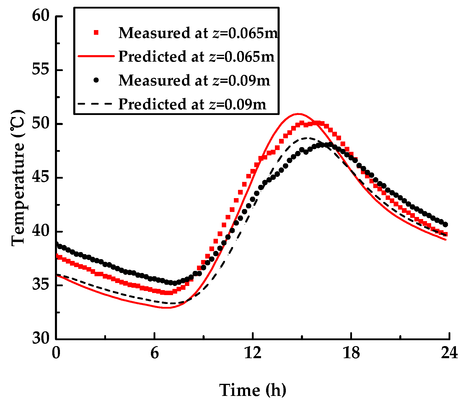
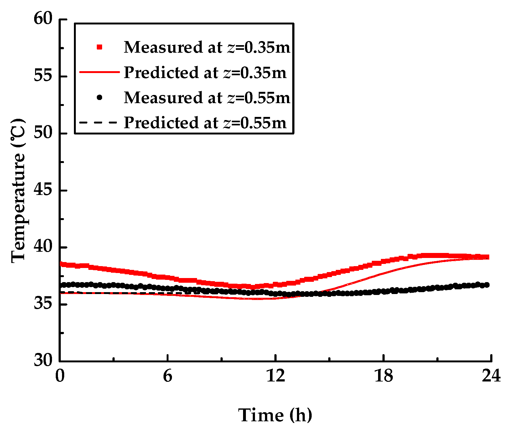
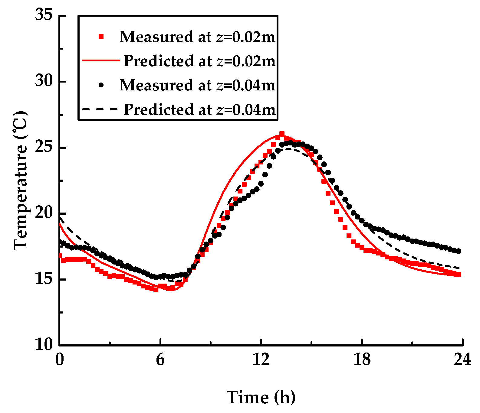
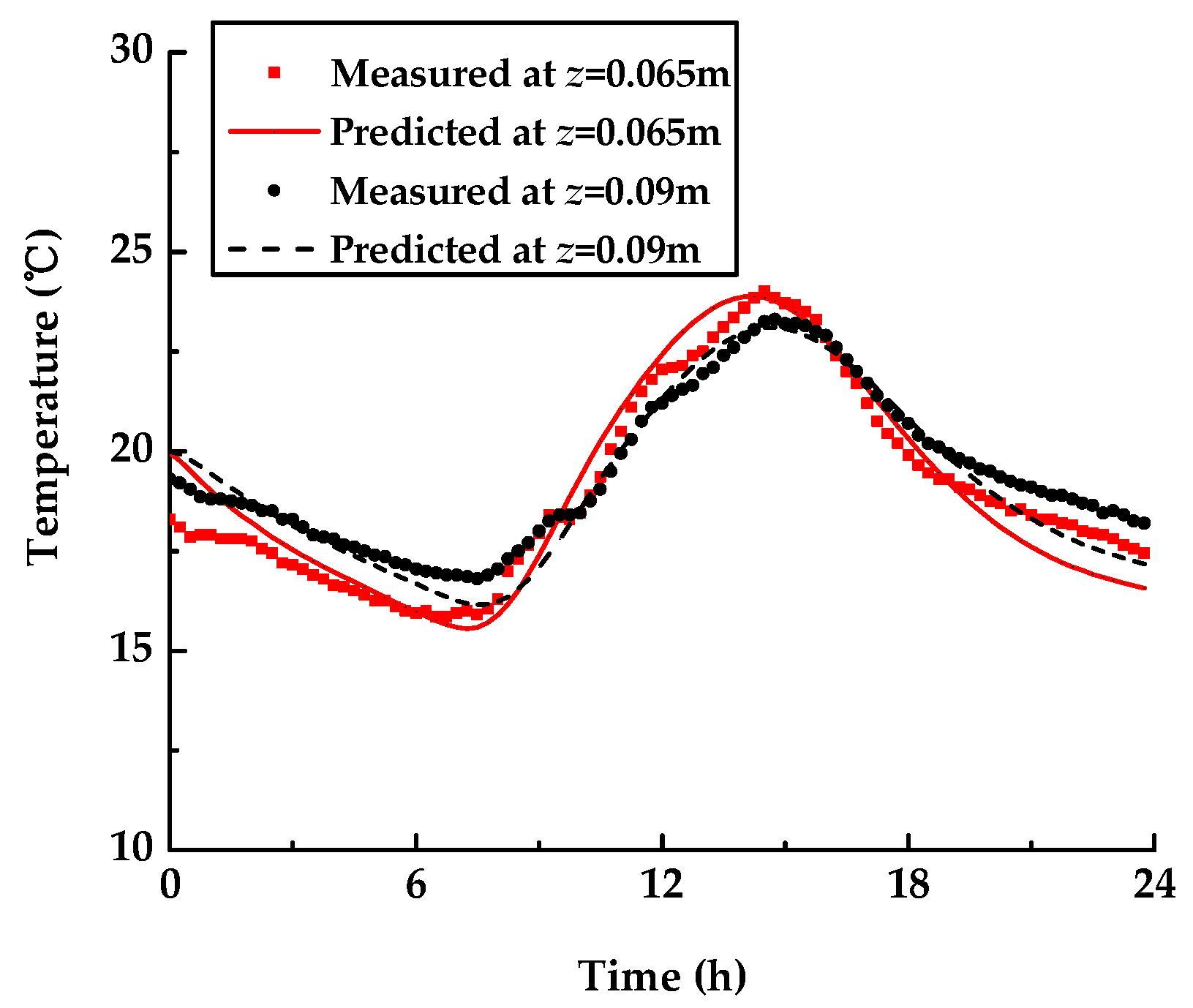
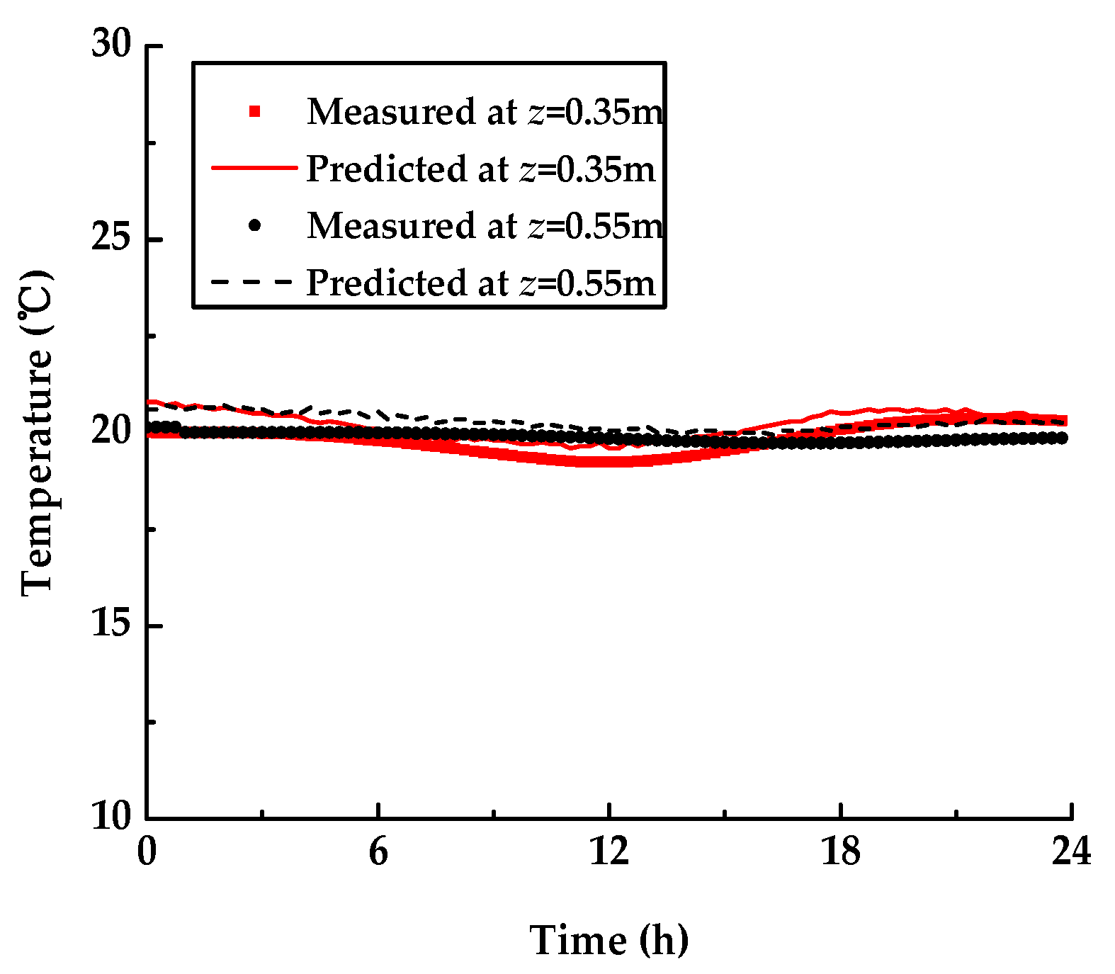
In order to measure temperature distributions throughout the pavement section, numerous temperature sensors were installed at different depths of the pavement section in this existing cement concrete pavement with an asphalt overlay. The measured and calculated pavement temperatures at z =0.02 m (at the middle of AC-13 layer), z = 0.04 m (at the bottom of AC-13 layer), z = 0.065 m (at the middle of AC-20 layer), z =0.09 m (at the bottom of AC-20 layer), z =0.35 m (at the bottom of C35 base) and z = 0.55 m (at the bottom of C20 subbase) are plotted every 15 min for a 24-h period in Figure 5, Figure 6 and Figure 7 for 24 August (summer) and Figure 8, Figure 9 and Figure 10 for 16 December (winter), respectively. From Figure 5, Figure 6, Figure 7, Figure 8, Figure 9 and Figure 10, the pavement temperatures predicted by the proposed solution match well with the measured temperatures.
Let and be the predicted and measured pavement temperature, respectively. Table 4 lists the maximum and minimum values of , the mean absolute error values, i.e. ,at six various depth positions during two different time periods (summer and winter).
From Table 4, the maximum absolute errors and the maximum mean absolute error values between the predicted and measured temperature at different depth locations are less than 2.89 °C and 1.58 °C, respectively. The increase in the pavement depth can lead to lower average relative absolute errors.
Therefore, the proposed analytical solutions derived by the technique of Laplace transform and its numerical inversion can be applied to conduct the prediction of the temperature distribution in the existing cement concrete pavement with an asphalt overlay with reasonable and high accuracy. The prediction error is caused by the assumed conditions of the model (e.g., the initial pavement temperature is assumed a constant), material property inputs (e.g., the convection coefficient is assumed a constant in one day) and the error of the measured data and the Laplace numerical inversion transform.
5. Conclusions
To obtain the one-dimensional distribution of the time-dependent temperature, the Gaussian quadrature equation was used to resolve the Laplace inverse transform and Laplace transform. Based on a system of multilayered pavements, this study subsequently came up with an analytical solution of this temperature field. Then, discrete least-squares approximations of the interpolatory trigonometric polynomials were used to fit several specific measured climatic factors regarded as the surface boundary conditions, i.e., the measured solar radiation intensity and air temperature. The solution process was simplified by the deduction of the relationship between the first layer and the constants of integration for the jth layer. The analytical solution can be obtained easily through solving the inverse Laplace transform using the Gaussian quadrature formula.
It can be obtained from the comparison between the predicted and measured temperatures that the maximum absolute errors and the maximum mean absolute error values in the existing cement concrete pavement with an asphalt overlay at various depth locations are below 2.89 °C and 1.58 °C, respectively, which means that the one-dimensional analytical solution proposed in this study can lead to a reasonable and highly accurate temperature distribution with time dependence for a period of 24 h in both summer and winter conditions. Further, the prediction of multilayered pavement temperature profiles can be promoted by this analytical solution based on the solar radiation intensities and air temperatures.
It is noted that the developed analytical temperature model was validated with relatively hot weather data. Future research will be conducted to validate the accuracy of the temperature prediction for pavements at a high latitude, where the local solar radiation is relatively sluggish and the local air temperature is relatively low.
Author Contributions
L.Z. and P.L. conceived the study and developed the analytical model; J.H. and L.Z. took part in field test and acquired the data; L.Z. and J.H. contributed to the data analysis and interpretation; J.H. also carried out the parameter estimations; and P.L. provided the required resources and validated results. All authors contributed to the writing, review and editing of the manuscript. All authors have read and agreed to the published version of the manuscript.
Funding
This research was funded by the Special Fund for Basic Scientific Research of Central Colleges, grant number 300102219519; The Guangdong Provincial Transportation Science and Technology Project, grant number 2017-02-003; The Science and Technology Project from the Affairs Center for Highway of Guangdong province, grant number 2017-15.
Conflicts of Interest
The authors declare that there is no conflict of interest.
References
- Chen, J.; Wang, H.; Xie, P. Pavement temperature prediction: Theoretical models and critical affecting factors. Appl. Therm. Eng. 2019, 158, 1–14. [Google Scholar] [CrossRef]
- Barber, E.S. Calculation of maximum pavement temperatures from weather reports. In Highway Research Board Bulletin, No. 168; National Research Council: Washington, DC, USA, 1957; pp. 1–8. [Google Scholar]
- Liang, R.Y.; Niu, Y.Z. Temperature and curling stress in concrete pavements: Analytical solution. J. Transp. Eng. 1998, 124, 91–100. [Google Scholar] [CrossRef]
- Liu, C.; Yuan, D. Temperature distribution in layered road structures. J. Transp. Eng. 2000, 126, 93–95. [Google Scholar] [CrossRef]
- Chong, W.; Tramontini, R.; Specht, L. Application of the Laplace transform and its numerical inversion to temperature profile of a two-layer pavement under site conditions. Numer. Heat Transf. Part A—Appl. 2009, 55, 1004–1018. [Google Scholar] [CrossRef]
- Wang, D.; Roesler, J.R. One-dimensional temperature profile prediction in multi-layered rigid pavement systems using a separation of variables method. Int. J. Pavement Eng. 2012, 15, 373–382. [Google Scholar] [CrossRef]
- Wang, D. Simplified analytical approach to predicting asphalt pavement temperature. J. Mater. Civ. Eng. 2015, 27, 04015043. [Google Scholar] [CrossRef]
- Wang, D.; Roesler, J.R.; Guo, D. Analytical approach to predicting temperature fields in multilayered pavement systems. J. Eng. Mech. 2009, 135, 334–344. [Google Scholar] [CrossRef] [Green Version]
- Wang, D.; Roesler, J.R. One-dimensional rigid pavement temperature prediction using Laplace transformation. J. Transp. Eng. 2012, 138, 1171–1177. [Google Scholar] [CrossRef]
- Wang, D. Analytical approach to predict temperature profile in a multilayered pavement system based on measured surface temperature data. J. Transp. Eng. 2012, 138, 674–679. [Google Scholar] [CrossRef]
- Wang, D. Prediction of time-dependent temperature distribution within the pavement surface layer during FWD testing. J. Transp. Eng. 2016, 142, 06016002. [Google Scholar] [CrossRef]
- Wang, D. Prediction of asphalt pavement temperature profile during FWD testing: Simplified analytical solution with model validation based on LTPP data. J. Transp. Eng. 2013, 139, 109–113. [Google Scholar] [CrossRef]
- Chen, J.; Li, L.; Zhao, L.; Dan, H.; Yao, H. Solution of pavement temperature field in environment-surface system through Green’s function. J. Cent. South Univ. Technol. 2014, 21, 2108–2116. [Google Scholar] [CrossRef]
- Chen, J.; Wang, H.; Zhu, H. Analytical approach for evaluating temperature field of thermal modified asphalt pavement and urban heat island effect. Appl. Therm. Eng. 2017, 113, 739–748. [Google Scholar] [CrossRef]
- Alawi, M.H.; Helal, M.M. Mathematical modelling for solving nonlinear heat diffusion problems of pavement spherical roads in Makkah. Int. J. Pavement Eng. 2012, 13, 137–151. [Google Scholar] [CrossRef]
- Qin, Y. Pavement surface maximum temperature increases linearly with solar absorption and reciprocal thermal inertial. Int. J. Heat Mass Transf. 2016, 97, 391–399. [Google Scholar] [CrossRef]
- Dumais, S.; Dore, G. An albedo based model for the calculation of pavement surface temperatures in permafrost regions. Cold Reg. Sci. Technol. 2016, 123, 44–52. [Google Scholar] [CrossRef]
- Burden, R.L.; Faires, J.D. Numerical Analysis, 7th ed.; Brooks/Cole: Pacific Grove, CA, USA, 2001. [Google Scholar]
- Zhu, B. Thermal Stress and Temperature Control of Mass Concrete; China Electric Power Press: Beijing, China, 1998. [Google Scholar]
- Davis, P.J.; Rabinowitz, P. Methods of Numerical Integration, 2nd ed.; Academic Press: Orlando, FL, USA, 1984. [Google Scholar]
- Stroud, A.H.; Secrest, D. Gaussian Quadrature Formulas; Prentice Hall: Upper Saddle River, NJ, USA, 1966. [Google Scholar]
- Heydarian, M.; Mullineux, N.; Reed, J. Solution of parabolic partial differential equations. Appl. Math. Model. 1981, 5, 448–449. [Google Scholar] [CrossRef]
- Zi, J.; Wang, H.; Li, F.; Zhou, W. Reflection cracking resistance stress analysis of large stone asphalt mixtures base in asphalt pavement. J. Huazhong Univ. Sci. Technol. 2006, 23, 8–12. [Google Scholar]
Figure 1.
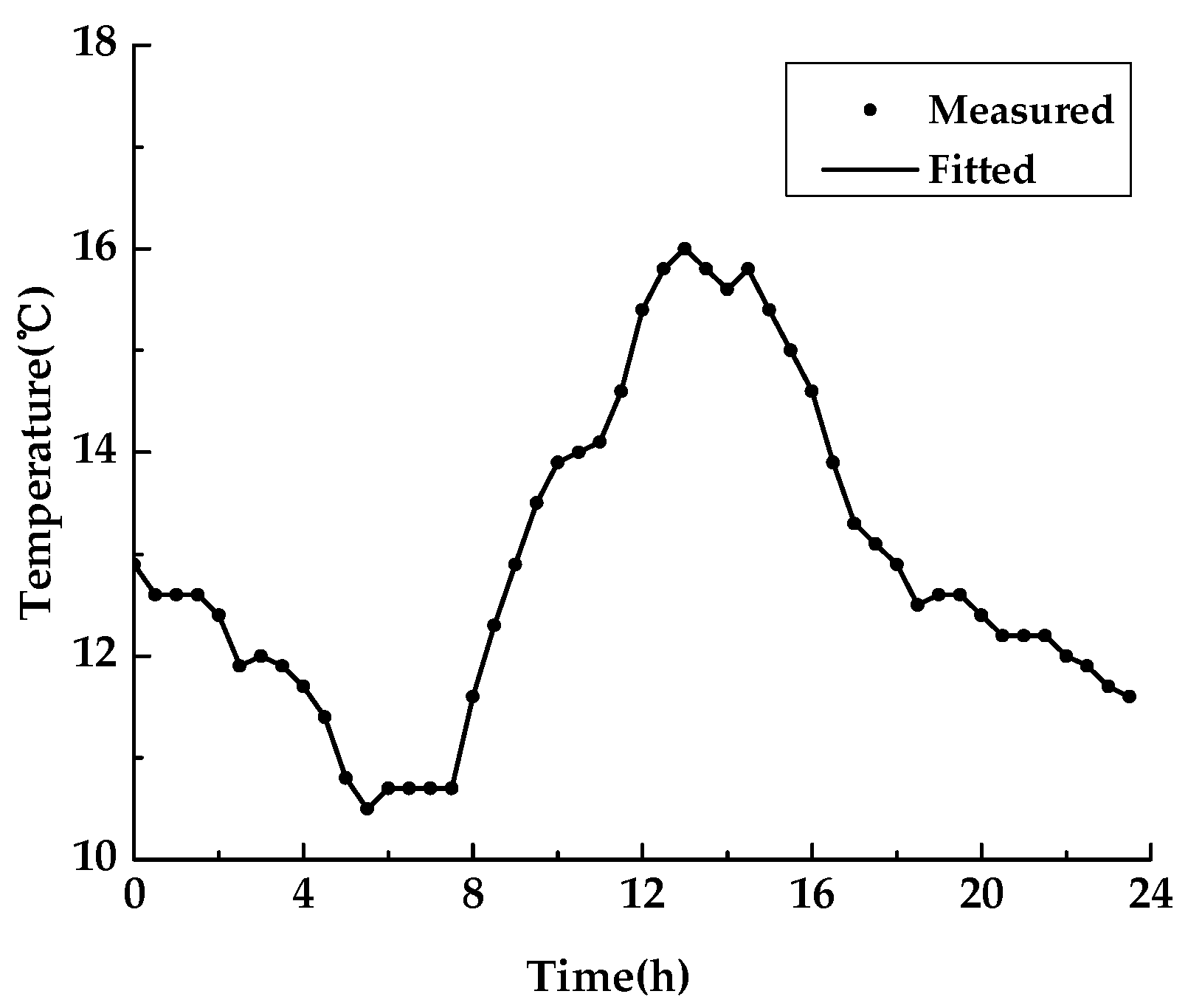
Measured and fitted air temperature on 24 August.

Figure 2.
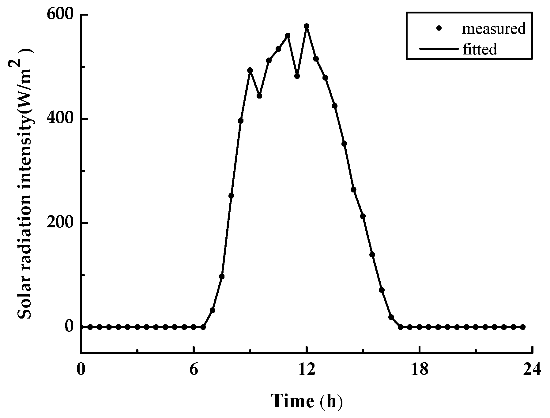
Measured and fitted solar radiation intensity on 24 August.

Figure 3.
Measured and fitted air temperature on 16 December.

Figure 4.
Measured and fitted solar radiation intensity on 16 December.

Figure 5.
Measured and predicted temperature at z =0.02 m and z = 0.04 m on 24 August.

Figure 6.
Measured and predicted temperature at z = 0.065 m and z = 0.09 m on 24 August.

Figure 7.
Measured and predicted temperature at z = 0.35 m and z = 0.55 m on 24 August.

Figure 8.
Measured and predicted temperature at z = 0.02 m and z = 0.04 m on 16 December.

Figure 9.
Measured and predicted temperature at z = 0.065 m and z = 0.09 m on 16 December.

Figure 10.
Measured and predicted temperature at z = 0.35 m and z =0.55 m on 16 December.


Table 1.
The Gaussian integration points () and the weight coefficients of the Gaussian integration points () values.
Table 1.
The Gaussian integration points () and the weight coefficients of the Gaussian integration points () values.
| 1 | 1.283767707781087 × 10 + i1.666062584162301 | −8.684606112670226 × 10² + i1.545742053305275 × 104 |
| 3 | 1.222613148416215 × 10 + i5.012719263676864 | 1.551634444257753 × 10³ − i8.439832902983925 × 103 |
| 5 | 1.093430343060001 × 10 + i8.409672996003092 | −8.586520055271992 × 10² + i2.322065401339348 × 103 |
| 7 | 8.776434640082609 + i1.192185389830121×10 | 1.863271916070924 × 10² − i2.533223820180114 × 102 |
| 9 | 5.225453367344361 + i1.572952904563926×10 | −1.03490190706237 × 10 + i4.110935881231860 |
Table 2.
Fitted parameters of the air temperatures and solar radiation intensities.
| Date | Fitted Parameters of Air Temperatures | Fitted Parameters of Solar Radiation Intensities | ||||
|---|---|---|---|---|---|---|
| Correlation Coefficient R2 | Correlation Coefficient R2 | |||||
| 24 August 2015 | 63.404 | −0.0458 | 0.999 | 364.625 | 4.791 | 0.999 |
| 16 December 2015 | 21.971 | 0.0625 | 0.999 | 285.708 | 9.458 | 0.999 |
Table 3.
The input parameters in the model verification.
| Pavement Structure | Thickness (m) | Thermal Conductivity (W/(m·°C)) | Thermal Diffusivity (m2/h) |
|---|---|---|---|
| AC-13 asphalt overlay upper layer | 0.04 | 1.5 | 0.0022 |
| AC-20 asphalt overlay lower layer | 0.05 | ||
| C35 cement concrete base | 0.26 | 1.4 | 0.0028 |
| C20 cement concrete subbase | 0.20 | ||
| Subgrade | - | 1.4 | 0.0030 |
Table 4.
Errors between the predicted and measured temperatures of various depth locations.
| Date | Error Type | Depth Location z (m) | |||||
|---|---|---|---|---|---|---|---|
| 0.02 | 0.04 | 0.065 | 0.09 | 0.35 | 0.55 | ||
| 24 August | (°C) | 1.84 | 2.05 | 1.73 | 1.40 | −0.12 | 0.03 |
| (°C) | −2.89 | −2.45 | −1.87 | −2.85 | −2.54 | −0.75 | |
| (°C) | 1.07 | 1.17 | 1.32 | 1.58 | 1.26 | 0.27 | |
| 16 December | (°C) | 2.43 | 1.89 | 1.66 | 0.77 | 0.00 | −0.20 |
| (°C) | −0.48 | −1.43 | −1.06 | −1.10 | −0.80 | −0.70 | |
| (°C) | 0.71 | 0.67 | 0.53 | 0.41 | 0.38 | 0.40 | |
© 2020 by the authors. Licensee MDPI, Basel, Switzerland. This article is an open access article distributed under the terms and conditions of the Creative Commons Attribution (CC BY) license (http://creativecommons.org/licenses/by/4.0/).
Share and Cite
MDPI and ACS Style
Zhang, L.; Huang, J.; Li, P. Prediction of Temperature Distribution for Previous Cement Concrete Pavement with Asphalt Overlay. Appl. Sci. 2020, 10, 3697. https://doi.org/10.3390/app10113697
AMA Style
Zhang L, Huang J, Li P. Prediction of Temperature Distribution for Previous Cement Concrete Pavement with Asphalt Overlay. Applied Sciences. 2020; 10(11):3697. https://doi.org/10.3390/app10113697
Chicago/Turabian StyleZhang, Lijuan, Jianwu Huang, and Peilong Li. 2020. "Prediction of Temperature Distribution for Previous Cement Concrete Pavement with Asphalt Overlay" Applied Sciences 10, no. 11: 3697. https://doi.org/10.3390/app10113697
Note that from the first issue of 2016, this journal uses article numbers instead of page numbers. See further details here.